Spatiotemporal variability and long-term trends of ocean acidification in the California Current System

(1)

Biogeosciences, 10, 193–216, 2013 www.biogeosciences.net/10/193/2013/ doi:10.5194/bg-10-193-2013

Biogeosciences

Spatiotemporal variability and long-term trends of ocean

acidification in the California Current System

C. Hauri1,6, N. Gruber1, M. Vogt1, S. C. Doney2, R. A. Feely3, Z. Lachkar1, A. Leinweber4, A. M. P. McDonnell1,6, M. Munnich1, and G.-K. Plattner1,5

1_{Environmental Physics, Institute of Biogeochemistry and Pollutant Dynamics, ETH Zurich, Zurich, Switzerland} 2_{Dept. of Marine Chemistry and Geochemistry, Woods Hole Oceanographic Institution, Woods Hole, MA, USA} 3_{Pacific Marine Environmental Laboratory/National Oceanic and Atmospheric Administration, Seattle, WA, USA} 4_{Institute of Geophysics and Planetary Physics, University of California, Los Angeles, CA, USA}

5_{Climate and Environmental Physics Group, Physics Institute, University of Bern, Bern, Switzerland} 6_{now at: School of Fisheries and Ocean Sciences, University of Alaska Fairbanks, Fairbanks, AK, USA}

Correspondence to:C. Hauri ([email protected])

Received: 6 July 2012 – Published in Biogeosciences Discuss.: 6 August 2012

Revised: 4 December 2012 – Accepted: 7 December 2012 – Published: 14 January 2013

Abstract.Due to seasonal upwelling, the upper ocean waters of the California Current System (CCS) have a naturally low pH and aragonite saturation state (arag), making this region particularly prone to the effects of ocean acidification. Here, we use the Regional Oceanic Modeling System (ROMS) to conduct preindustrial and transient (1995–2050) simulations of ocean biogeochemistry in the CCS. The transient simula-tions were forced with increasing atmosphericpCO2and in-creasing oceanic dissolved inorganic carbon concentrations at the lateral boundaries, as projected by the NCAR CSM 1.4 model for the IPCC SRES A2 scenario. Our results show a large seasonal variability in pH (range of∼_{0.14) and}arag (∼_{0.2) for the nearshore areas (50 km from shore). This}

vari-ability is created by the interplay of physical and biogeo-chemical processes. Despite this large variability, we find that present-day pH andaraghave already moved outside of their simulated preindustrial variability envelopes (defined by ±_{1 temporal standard deviation) due to the rapidly}

in-creasing concentrations of atmospheric CO2. The nearshore surface pH of the northern and central CCS are simulated to move outside of their present-day variability envelopes by the mid-2040s and late 2030s, respectively. This transition may occur even earlier for nearshore surfacearag, which is projected to depart from its present-day variability envelope by the early- to mid-2030s. The aragonite saturation horizon of the central CCS is projected to shoal into the upper 75 m within the next 25 yr, causing near-permanent

undersatura-tion in subsurface waters. Due to the model’s overestimaundersatura-tion of arag, this transition may occur even earlier than simu-lated by the model. Overall, our study shows that the CCS joins the Arctic and Southern oceans as one of only a few known ocean regions presently approaching the dual thresh-old of widespread and near-permanent undersaturation with respect to aragonite and a departure from its variability en-velope. In these regions, organisms may be forced to rapidly adjust to conditions that are both inherently chemically chal-lenging and also substantially different from past conditions.

1 Introduction

(2)

scientific research (Doney et al., 2012), many (although not all) results have demonstrated that these changes can have deleterious effects on marine-calcifying invertebrates such as corals, coralline algae, oyster larvae and pteropods (Orr et al., 2005; Kleypas et al., 2006; Martin and Gattuso, 2009).

The California Current System (CCS) has a naturally low pH and aragonite saturation state (arag), making it particu-larly prone to the effects of ocean acidification (Feely et al., 2008; Gruber et al., 2012). Seasonal upwelling is induced by equatorward winds in early spring. The upwelling brings cold subsurface water, rich in nutrients and dissolved inor-ganic carbon (DIC), up to the surface. The high DIC con-tent of the upwelled waters endows them with a low pH and arag. Once close to the surface, the nutrient-rich water trig-gers the onset of phytoplankton blooms that then draw down oceanicpCO2to levels sometimes below atmosphericpCO2 (Hales et al., 2005), causing an increase in surface water pH andarag. Conversely, remineralization processes of sinking organic matter counteract the effects of production by lower-ing pH andarag. Physical circulation can affect the duration and magnitude of these biological processes and therefore plays an important role in controlling the evolution and spa-tial pattern of pH andarag.

These physical and biological features create large spa-tial and temporal variability in pH and arag in the CCS (Feely et al., 2008; Juranek et al., 2009; Alin et al., 2012). North of Point Conception (34.5◦N), a combination of strong seasonal upwelling events and remineralization trigger a pH drop to 7.65 andaragto 0.8 at the surface in some nearshore environments (Feely et al., 2008). Combined with high bio-logical production, a heterogeneous distribution of pH and arag is created. Offshore pH andaragare not directly in-fluenced by upwelling and remain above 8.0 and 2.2, respec-tively. Reconstructed pH andaragfrom temperature (T) and oxygen (O2) time series from the central Oregon shelf dis-play a seasonal range ofarag of 0.8–1.8 at 30 m (Juranek et al., 2009), with lowest levels attained during the upwelling season between spring and fall. South of Point Conception, upwelling-favorable winds are weaker, yet more persistent throughout the year (Dorman and Winant, 1995). In contrast to the area north of Point Conception, reconstructed pH and aragfromT and O2time series display the highest levels in summer, due to biological drawdown of CO2in warm subsur-face waters (30 m). Spatial variability is also highest in sum-mer, most likely driven by an interplay of high productivity and upwelling (Alin et al., 2012). At the Santa Monica Bay Observatory (SMBO at 33◦_55.9′_{N and 118}◦_42.9′_W),

sur-face pH andaragdisplay a large seasonal variability, rang-ing by±_{0.08 (1 STD) and}±_{0.4 units, respectively}

(Leinwe-ber and Gru(Leinwe-ber, 2013).

In the CCS, the aragonite saturation horizon has shoaled 50–100 m since the preindustrial era (Feely et al., 2008; Hauri et al., 2009; Juranek et al., 2009) and will continue to rise in response to future oceanic uptake of anthropogenic CO2. Simulations forced with increasing atmosphericpCO2

– as projected by the NCAR CSM 1.4 model run under the IPCC SRES A2-scenario (Naki´cenovi´c and Swart, 2000) – suggest that about 70 % of the euphotic nearshore region of the central US West Coast will become undersaturated with regard to aragonite ( <1) during the upwelling season by 2050. Within the next 20 to 30 yr this “absolute” threshold of aragonite undersaturation will be reached throughout the year in nearly all habitats along the seafloor (Gruber et al., 2012).

Due to the large “natural” variability of pH andarag, it is conceivable that the organisms of the CCS are not only well adjusted to low levels of pH and arag, but also to a large range of chemical conditions. Therefore, in order to evaluate the impact of ocean acidification, it is also neces-sary to consider how the chemical conditions evolve in re-lationship to this “natural”variability. Eventually, the anthro-pogenic trend of ocean acidification will drive the waters to-ward levels of pH and arag that are well below those the organism experienced in the preindustrial era. Assuming that the organisms’ tolerance for low pH andaragconditions de-creases rapidly once it lives below these “natural” levels, we define a “relative” threshold, i.e., by determining how and when future trajectories of pH andaragbegin to depart in a significant manner from current and prior conditions. Coo-ley et al. (2012) and Friedrich et al. (2012) have used global Earth System Models to study this relative threshold. How-ever, their coarsely resolved models are not able to simulate many important local to regional processes, such as coastal upwelling. This in turn leads in these models to an overes-timation of pH andaraglevels, an underestimation of their temporal and spatial variability, and hence large potential er-rors in the timing of the crossing of the absolute and relative thresholds.

Here, we use regional model simulations to describe the spatiotemporal variability of pH andaragin the CCS from the Mexican to the Canadian border, and project their fu-ture evolution until 2050 using two emissions scenarios. We will investigate whether the CCS, despite its high variability, is projected to approach the combined absolute and relative thresholds of both chemical dissolution of aragonite and a de-parture from the variability envelopes of pH andarag.

2 Methods

2.1 Model setup

(3)

C. Hauri et al.: Variability and long-term trends of ocean acidification 195

curvilinear coordinates and a terrain-following vertical co-ordinate (σ) with 32 depth levels, with enhanced resolution near the surface and nearshore on the shallow shelf (see Gru-ber et al., 2011; Lachkar and GruGru-ber, 2011, for a detailed description of the model setup).

The biogeochemical model used here is a simple nitrogen-based NPZD2 and is described in detail in Gruber et al. (2006). The analyzed simulations are those presented in Gru-ber et al. (2012) and use the same biogeochemical parameters as those employed by Lachkar and Gruber (2011). The model considers six pools of nitrogen, i.e., nitrate (NO−₃) and am-monium (NH+₄), phytoplankton, zooplankton and two types of detritus. The large detritus pool sinks fast (10 m day−1) and the smaller one sinks at a slower rate (1 m day−1). How-ever, the small detritus pool coagulates with a fraction of phy-toplankton to form large detritus, which increases its sinking speed.

The carbon component of the model adds three new state variables to the biogeochemical model, i.e., DIC, Alkalinity (Alk) and mineral CaCO3. It is not necessary to add explicit carbon-based state variables to the organic pools, i.e., phyto-plankton, zooplankton and the two detrital pools, since they are all assumed to have a fixed C:N stoichiometric ratio of 106:16 (Redfield et al., 1963). This also implies that biolog-ically mediated processes with the exception of the biogenic formation of CaCO3are assumed to have this stoichiometry as well. DIC is modified by gas exchange, CaCO3 precipita-tion and dissoluprecipita-tion, and net community producprecipita-tion, which is net primary production minus heterotrophic respiration. Alk is primarily governed by the precipitation and dissolution of CaCO3. But Alk is also changed by the generation of NO−₃ through nitrification and its removal by new production. The biogenic CaCO3formation is tied to net primary production with a fixed production ratio of 7 % (Sarmiento et al., 2002; Jin et al., 2006), i.e., for each mole of organic carbon formed by NPP, 0.07 mol of CaCO3is formed. CaCO3dissolves at a constant dissolution rate of 0.0057 day−1_{and sinks at a} ve-locity of 20 m day−1_{, which is twice the sinking velocity of} large detritus. OceanicpCO2is calculated from DIC, Alk,T and salinity (S) using the standard OCMIP carbonate chem-istry routines1. The routines used the carbonic acid dissoci-ation constants of Mehrbach et al. (1973), as refit by Dick-son and Millero (1987) and DickDick-son (1990). The pressure effect on the solubility was taken from Mucci (1983), in-cluding the adjustments to the constants recommended by Millero (1995). Gas exchange is parameterized following Wanninkhof (1992), with the gas transfer velocity depend-ing on the square of the wind speed. The reader interested in a more detailed description of the carbon biogeochemistry module is referred to Appendix A.

1_{http://ocmip5.ipsl.jussieu.fr/OCMIP/}

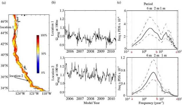
Fig. 1.Map of the domain of the US West Coast configuration of ROMS. The northern subregion is defined by the dark blue box and represents the area between the northern boundary of 47.5◦N and a southern boundary at Cape Mendocino (40.5◦N). Between Cape Mendocino and Point Conception (34.5◦N) the central sub-region is defined by the orange box. The southern subsub-region ex-tends southward from Point Conception to 32.4◦N. The light blue line defines the study area of 50 km along the coast. Because of the perpendicular orientation of the regional boundaries, the offshore part of each region’s lower boundary lays south of the above men-tioned latitudes. The yellow dots indicate the locations used in the model-observational data spatial comparison (see Sect. 3). The ar-row is pointed at the transect used for visual comparison. The Santa Monica Bay Observatory Mooring (33◦55.9′N and 118◦42.9′W) is shown as a red dot.

2.2 Forcing

(4)

momentum fluxes computed from QuickSCAT-based Scat-terometer Climatology of Ocean Winds (SCOW, Risien and Chelton, 2008). The surface heat and freshwater fluxes were derived from the Comprehensive Ocean-Atmosphere Data Set (COADS) data products (da Silva et al., 1994) and ap-plied with surface T and S restoring after Barnier et al. (1995) with a relaxation timescale of three months. To a lim-ited extent, this approach allows implicitly taking into ac-count riverine-driven seasonal variability of S associated with the Columbia River, even though riverine input is not explicitly modeled. The initial and boundary conditions for T,S and nutrients were taken from the World Ocean Atlas 2005 (WOA05)2. Monthly means of WOA05 were also used to prescribeT,S, and momentum fluxes along the three lat-eral open boundaries following a radiative scheme (March-esiello et al., 2003). Initial and boundary conditions for DIC and Alk were taken from the GLobal Ocean Data Analysis Project (GLODAP, Key et al., 2004). A seasonal cycle was introduced in the DIC and Alk boundary conditions using a monthly climatology ofpCO2(Takahashi et al., 2006) and a monthly climatology of surface Alk, calculated usingT and Sfollowing Lee et al. (2006). These seasonal DIC and Alk variations are assumed to occur throughout the upper 200 m, but are attenuated with depth by scaling them to the vertical profile of the seasonal amplitude ofT. After a model spin-up of 10 yr, the transient simulation was forced with increasing pCO2 from 364 ppm in 1995 to 541 ppm in 2050, and in-creasing DIC concentrations at the lateral boundaries. These atmospheric and lateral boundary conditions were taken from a simulation of the fully coupled Earth System Model NCAR CSM 1.4 (Frölicher et al., 2009), which was forced with the SRES A2 emissions scenario (Nakićenović and Swart, 2000). While the atmosphericpCO2was taken directly from the NCAR model, the lateral DIC concentrations were deter-mined by combining the present-day DIC field from GLO-DAP and adding to them the annual increment of DIC from the NCAR CSM 1.4 carbon model simulation. DIC and at-mospheric pCO2 at the lateral boundaries were the only forcings that changed over the years, while the atmospheric physical forcings, as well as the lateral boundary conditions of Alk,T,S, nutrients and circulation remained unchanged from their seasonal climatologies for the entire simulation from 1995 to 2050. For the preindustrial time-slice simula-tion, the atmosphericpCO2was set to a preindustrial value of 280 ppm, and the lateral DIC boundary conditions were taken from the preindustrial fields of GLODAP (Key et al., 2004).

In order to analyze the sensitivity of our results toward the chosen SRES emissions scenario, we compared the results of two additional transient simulations that follow both the “high-CO2” SRES emissions scenario A2 described above, and the “low-CO2” SRES emissions scenario B1 (Figs. A2 and A3). Due to computational constraints, these two

addi-2_{http://www.nodc.noaa.gov/OC5/WOA05/pr woa05.html}

tional simulations were conducted with a coarser-resolution setup of 15 km (Gruber et al., 2012). By 2050, atmospheric pCO2increased to 492 ppm in the B1 scenario, compared to 541 ppm in the A2 scenario.

2.3 Study area

As our primary interest is the nearshore area, we largely re-stricted our analyses to the first 50 km in an east–west di-rection along the coast (Fig. 1, within light blue line). With regard to depth, we analyzed pH and arag at two distinct depths, i.e., the surface and 100 m, in order to retain the full spatial variability of pH andarag, which would have been lost by averaging over the euphotic zone. We also divided the CCS into three subregions defined by Dorman and Winant (1995), based on distinct regional differences in the wind and temperature patterns that potentially affect the dynam-ics of pH andarag. The region north of Cape Mendocino (40.5◦N) is subsequently denoted as the “northern” (blue), the region between Cape Mendocino and Point Conception (34.5◦N) as the “central” (orange) and the region south of Point Conception as the “southern” (red) subregion (Fig. 1).

2.4 Temporal resolution of model output

Our analyses of the modeled evolution of pH andaragfrom 2005 to 2050 are based on monthly averages, with the tem-poral resolution primarily having been determined by com-putational and storage constraints. Although such a monthly time averaging reduces the aliasing of unresolved timescales that would result from the analysis of monthly time-slices, it fails to capture the full variability. In order to determine the degree to which the monthly averages represent the full variability, we conducted a spectral analysis of the two-day model output that we had generated for a limited time period only (2006–2010). Such a two-day output captures nearly all of the variability in our model, because in our climatologi-cally forced simulations, all of the simulated high-frequency variability is driven by mesoscale processes with character-istic time scales of between a few days and several weeks.

For the spectral analysis, we calculated the Welch power density spectrum (PDS) of the Fourier transform of the de-trended time series data from each grid cell using a Hann window (Glover et al., 2011). The interval for the frequencies (f) captured with monthly output was set toa=_{0.2 yr}−1_and

tob=6 yr−1_{, according to thresholds given by the Nyquist–} Shannon sampling theorem. For the frequencies captured with two-day output, the upper boundary was set to c=

90 yr−1_{. We quantified the amount of total variability across} all frequencies fromatocand compared it to the amount of variability occurring in the frequencies froma tob. We de-fineMas the percentage of the total variability of surface pH oraragthat occurs at frequencies less thanbas follows:

M= Rb

aPDS(f )df Rc

a PDS(f )df

(5)

A plot ofM at the surface (Fig. 2a) reveals that in most areas (98.5 %) along the US West Coast, the majority of variability of surface-modeled pH and arag occurs at fre-quencies less thanband can be captured by monthly model output. However, as will be discussed in Sect. 4.1, high-frequency variability can lead to very low pH andarag in some nearshore surface areas. These few areas are limited to about 1.5 % of the nearshore 50 km along the US West Coast. There, less than 50 % of the total variability of surface pH can be captured with monthly model output (Fig. 2a, blue).

The time series (Fig. 2b) and the PDS of the Fourier transform (Fig. 2c) of two distinct example locations rep-resent these two extreme cases: in location 1 (43◦35′N, 124◦45′W), the monthly averaged sampling frequency cap-tures 89 %, whereas in location 2 (35◦₂₉′_{N, 121}◦₃₄′_W),

only 49 % of the total variability of surface pH is captured with monthly modeled means. While in location 1 low-frequency variability dominates (Fig. 2c, upper panel), high-frequency variability prevails in location 2 (Fig. 2c, lower panel).

At 100-m depth, the majority of variability of modeled arag occurs at frequencies less than b (Fig. 3a). Thus the low-frequency variability of arag is the most dominant mode along the entire US West Coast (Fig. 3c) and can be very well captured by the monthly averages.

To account for areas where the model variability of pH and aragare not fully captured with monthly average output, we introduce a correction factor (varcf):

varcf= v u u tσ 2 two-day

σ_month2 , (2)

whereσ_two-day2 is the temporal variance of the two-day output of model year 2010 andσ_month2 is the temporal variance of the monthly averaged, two-day output data of the same year. The correction factor varcfvaries between 1.2 in the northern and southern CCS and 1.4 in the central CCS and is used to correct the variability envelopes in Sect. 4.4.

Additional high-frequency variability, such as due to syn-optic wind-driven upwelling events, for example, cannot be captured with either model output type due to our choice of monthly climatological wind forcing (see Sects. 3 and 5 for further discussion).

3 Model evaluation

The model’s performance for simulating observed sea sur-face T, surface chlorophyll and the mixed layer depth was already evaluated in Lachkar and Gruber (2011) and Gruber et al. (2006, 2011). The model simulates the ob-served annual and seasonal patterns of surface tempera-ture well with correlations ofρ= 0.98 andρ= 0.95, respec-tively. It also captures successfully the offshore extent of the cold upwelling region. The modeled annual mean

mixed-layer depth has a correlation of 0.70 with observational data, but has a substantially higher standard deviation relative to the observations. The annual mean pattern of chlorophylla compares well with the SeaWiFS data set (ρ= 0.80), but the model underestimates chlorophyll a in the nearshore 100 km and has a poorer representation of its seasonal cycle (ρ= 0.46). The current paper will supplement these earlier evaluations by comparing the model to in situ data with an emphasis on vertical and cross-shore variability of the key carbonate chemistry properties in the upper ocean (also see Gruber et al., 2012).

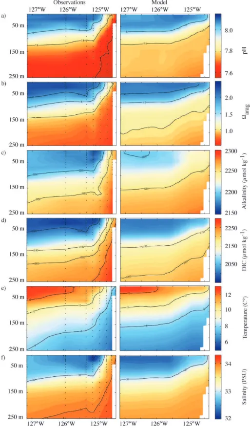
First, we evaluate the modeled spatial variability of pH, arag, DIC, Alk,T andSby comparing it to data from the North American Carbon Program (NACP) West Coast Cruise (Feely et al., 2008) (Fig. 1, yellow dots, lines 4–11). The ob-servational data were sampled between May and June 2007. For the comparison, we averaged model output of May and June from 2006 through 2010 and linearly interpolated it to a vertical grid with 1 m resolution. The model data were av-eraged over this 5-year period in order to remove any model-based interannual variability that could bias the results of the model evaluation.

A visual comparison of the modeled versus observed ver-tical distributions of the studied variables, along a represen-tative transect line (off Pt. St. George, California, Fig. 1, yellow arrow), indicates that the offshore pattern between 0 and 100 m is captured well (Fig. 4). However, the model underestimates the magnitude of the vertical difference of DIC (∼_{20 µmol kg}−1_{) in waters deeper than}∼_{125 m. In the}

nearshore region between 0 and 250 m depth, the model un-derestimates Alk by 10–35 µmol kg−1 _{and especially DIC} by 40–150 µmol kg−1_{. The larger bias (b) in DIC is the} primary cause of the overestimation of the simulated pH (bpH ∼0.2) and arag (barag ∼0.5), since their

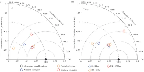
sensitivi-ties toward changes in Alk and DIC are similar. As a result, our modeled aragonite saturation horizon is typically 60 m deeper than the observed one, and up to 150 m deeper dur-ing the strongest upwelldur-ing events. There is no obvious dif-ference in model performance between subregions, i.e., pH andaragare modeled equally well for all three subregions, with a Pearson correlation coefficient of aboutρpH=_0.89–

0.90 between observed and modeled pH andρarag =0.88–

0.90 forarag(Fig. 5). The normalized standard deviations, correlation coefficients and biases between all observed and modeled properties can be found in Table A2.

(6)

Fig. 2.Analysis of variability of surface pH.(a)indicates the percentage of the total variability of surface pH that occurs at frequencies less thanb=6 yr−1. The arrows point out the locations of the two example sites described in panels(b)and(c).(b)Time series of surface pH over 5 yr for two distinct example locations and(c)a variance-conserving plot of the frequency×power density spectrum (PDS) vs. the frequency of the Fourier transformed time series. The black solid line represents the PDS and the black dashed lines envelope the±95 % confidence interval. The red dashed lines show the boundariesa,bandcof the integrals applied in Eq. (1).

Fig. 3.Analysis of variability ofaragat 100 m.(a)indicates the percentage of the total variability ofaragat 100 m that occurs at frequencies less thanb=6 yr−1. The arrows point out the locations of the two example sites described in panels(b)and(c).(b)Time series ofaragat

(7)

(8)

Fig. 5.Taylor diagram (Taylor, 2001) of model simulated(a)pH and(b) aragcompared to observations (Feely et al., 2008). A

five-year average of parameters over May and June (2006–2010) are compared to observations sampled between May and June 2007, for all sampled locations (black), the northern (blue circle), central (orange circle), and southern subregions (red circle), and for 0–100 m (blue diamond), 100–250 m (orange diamond) and 500–5000 m (red diamond). The distance from the origin is the normalized standard deviation of the modeled parameters. The azimuth angle represents the correlation between the observations and the modeled parameters The distance between the model point and the observation point (filled ellipse on the abscissa) indicates the normalized root mean square (RMS) misfit between model and observational estimates.

Gruber et al. (2006, 2012); Lachkar and Gruber (2011) and we focus on the implications of this discrepancy in the Dis-cussion.

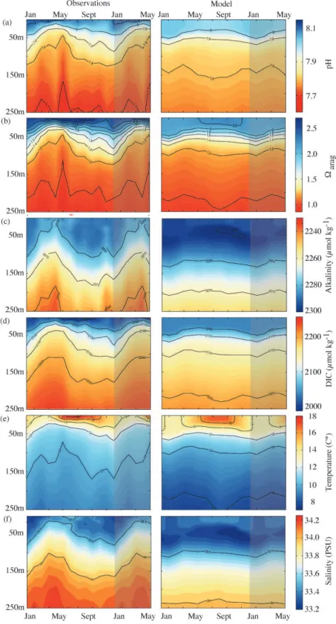
We evaluate the temporal variability of pH, arag, Alk, DIC, T and S by comparing our model results to a sea-sonal climatology from the Southern California Bight, gen-erated from roughly bi-weekly samples obtained from the Santa Monica Bay Observatory Mooring at 33◦_55.9′_{N and}

118◦42.9′W from 2003 to 2008 (Leinweber and Gruber, 2013). The model-based climatology for the same site and time-period underestimates pH and arag at depth (Fig. 6) as evidenced already in the comparisons with the NACP West Coast Cruises. In addition, the observations show high temporal variability at the surface (σpH=0.08, 1 STD for the full observational record andσarag=0.40) and at depth

(σpH=_{0.07 and}σarag =0.20), which is underestimated by

the model by a factor of about 7 for surfacearag and by a factor of about 3.5 for surface pH and both variables at 100 m. The observed high spatial and temporal variability of pH and arag of the southern CCS is dominated by high-frequency winds (Capet et al., 2004) that are not resolved in our current forcing files. Moreover, in the model, the bottom topography is smoothed over the continental shelf to prevent numerical instabilities associated with complex bathymetry. Therefore, the variability resulting from the interaction of the flow field with the observed bathymetry, particularly in the southern CCS, is not fully represented.

Better agreements with the observed temporal variabil-ity is achieved by the model for most other regions for

which data are available. A comparison with new pH and aragdata derived from a surface mooring off Newport, OR (44◦38′0′′N 124◦18′13′′W, Harris et al., 2013) from 2009 to 2011 demonstrates that the modeled temporal variabil-ity (σpH=0.10 and σarag=0.32, 1 STD) agrees well with

the observed temporal surface variability (σpH=0.11 and σarag=0.37, 1 STD). Also, the model is in better agreement

with the temporal variability of pH andaragin nearshore subsurface regions just north of Point Conception (Alin et al., 2012) than in the southern CCS. Alin et al. (2012) estimated pH andaragbased on seasonal hydrographic data from Cal-COFI line 76.7 from 2005 to 2010. Their estimated tempo-ral variability ofσpH=0.09 andσarag=0.32 at 30 m depth

are by a factor of 1.2 and 1.5, respectively, greater than the modeled temporal variability (σpH= 0.07 andσarag= 0.21).

The model-data misfit increases with depth. At 100 m depth, the model underestimates the temporal variability ofaragby a factor of 2 and by a factor of 5.5 for pH.

(9)

Fig. 6.Comparison of bi-weekly observed (2003–2008; Santa Monica Bay Observatory Mooring) and model simulated climatologies of(a) arag,(b)pH,(c)alkalinity,(d)DIC,(e)temperature and(f)salinity at 0–250 m between 2005 and 2010. The shaded area depicts the first

(10)

model evaluation and should be revised once additional ob-servational data are available.

4 Results

Here, we discuss the range and magnitude of changes in pH and arag and explore the drivers and mechanisms of the temporal and spatial variability in the nearshore environment of the CCS. We then present projections of the evolution of pH andaraguntil 2050 and determine the timing of when the chemical characteristics within the different subregions move outside of their modeled preindustrial and present-day variability envelopes (relative threshold). Finally, we project when the absolute threshold of aragonite undersaturation is reached.

4.1 Spatial and temporal patterns of modeled pH and

_arag

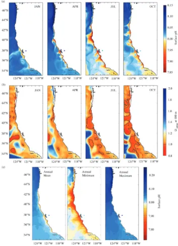
Examples of the modeled monthly averages for surface pH of model year 2011 (pCO2∼_{395 ppm) show that the waters}

within the first 50 km of the CCS experience a wide range of surface pH from 7.85 to 8.15 (Fig. 7a). Spatial variability of surface pH is highest in the central subregion (σpH=0.10, 1 STD) around July, while it is small and constant in the southern subregion (Fig. 8a and b). In the central nearshore CCS, the lowest surface pH (pHmin=_{7.85) is simulated}

be-tween June and September. The highest nearshore surface pH (pHmax=_{8.15) is reached between November and March in}

the northern subregion, while the central CCS only experi-ences high surface pH (pHmax=8.05) during three months (January–March). In the central CCS, surface pH decreases to 7.95 around June and increases to around 8.05 in January. Farther off the coast, surface pH of the northern subregion remains at around 8.10, while in the central and southern CCS it drops from 8.15 to 8.00. At 100 m depth, low pH of about 7.75 extends to about 300 km offshore all year round and in the entire CCS, except along the Washington coast, where pH remains close to about 8.10 between April and July, and drops to about 7.65 between August and October (not shown).

The seasonal evolution of surfacearag (not shown) be-haves similarly to surface pH. The modeled monthly means do not show undersaturation at the surface. However, model results from averaged two-day model output reveal that north of Cape Mendocino, surface pH can drop down to 7.72 (Fig. 7c) and surfacearag to 0.93, below the values cap-tured by the monthly mean outputs. In nearshore areas at 100 m depth, aragonite undersaturation is also simulated in late fall, most likely due to the remineralization of the sinking organic matter that was produced during the summer phy-toplankton blooms (Fig. 7b). Spatial variability of both pa-rameters and along the entire US West Coast is constant and small (Fig. 8a and b).

Fig. 7.Simulated monthly averages of(a)surface pH and(b)arag

at 100 m. Shown are January, April, July and October of model year 2011 (∼395 ppm atmospheric pCO2). (c)Mean, minimum

and maximum values of surface pH from two-day model output.

4.2 Spatially averaged seasonal cycle of pH and_arag_{for each subregion}

The range of the mean seasonal cycle of pH andaragvaries from region to region in the CCS (Fig. 8a and b) and is more pronounced at the surface than at 100 m. The northern sub-region has the highest annual mean surface pH (pH=_8.07)

and the most distinct seasonal cycle (Fig. 8a), with a range of about 0.14 pH units. In the central and southern CCS, the average surface pH is pH = 8.00 with a range of 0.09 and 0.04, respectively. While surface pH is lowest in August and September in the northern subregion, the central subregion shows the lowest surface pH (pHmin=_{7.95) in June.}

(11)

Fig. 8.Seasonal cycle of (a)pH and(b) aragin the nearshore

50 km. The lines represent the mean and the shaded area the spatial variability (±1 STD) for each month, for the northern (blue), cen-tral (orange) and southern (red) subregions, at the surface (left) and at 100 m (right). The shaded area depicts the first six months of the following annual cycle.

At 100 m depth, average pH remains around 7.8 and aver-agearagaround 1.1 in all three subregions.

4.3 Mechanisms influencing the seasonal cycle in pH and_arag

To understand the mechanisms causing the seasonal changes in pH andaragacross the three subregions, we investigate their sensitivity to the seasonal variations in Alk, DIC,T and S. To do so, we estimate the contribution of changes in each property to the total change of pH andarag. The change in pH andaragcan be “separated” using a Taylor expansion in first order of all considered variables:

1pH= ∂pH

∂DIC1sDIC+ ∂pH

∂Alk1sAlk+ ∂pH

∂T 1T (3)

+_1FSpH+_Res,

where

1FSpH=∂pH

∂S 1S+ ∂pH ∂DIC1DIC

s₊ ∂pH ∂Alk1Alk

s

(4) and

1= ∂

∂DIC1sDIC+ ∂

∂Alk1sAlk+ ∂

∂T1T (5)

+_1FS+_Res,

where 1FS=

∂ ∂S1S+

∂ ∂DIC1DIC

s₊ ∂ ∂Alk1Alk

s_.

(6) The partial derivatives quantify the differential changes in carbon chemistry due to small changes in DIC, Alk,T andS and are derived from model equations and annual means of

a modeled climatology (2006–2010).1sDIC and1sAlk are the salinity normalized deviations from the annual means of DIC and Alk;1DICsand1Alksare deviations from the an-nual means due to freshwater input, and1FSpHand1FS are the total contributions of freshwater input to the change in pH andarag, respectively. Residuals (= Res.) capture the error when the left- and right-hand side of the equation are not equal.

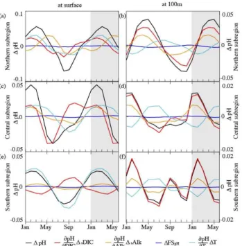
The seasonal variations in pH and arag are driven by a combination of seasonal changes in DIC, Alk andT. These parameters are altered by upwelling and eddies, which dif-fer in magnitude and timing from region to region (Figs. 9 and 10). In addition, Alk changes due to the precipitation or dissolution of CaCO3, and due to nitrification and ni-trate assimilation during new production (see Sect. 2.1, Ap-pendix A). DIC changes due to CaCO3calcification and dis-solution, net primary production and heterotrophic respira-tion. Surface temperature reflects changes in the incoming solar radiation and heat exchange with the atmosphere. Fig-ures 9 and 10 show the contributions of changes in DIC, Alk, SandT to changes (relative to the annual mean) in pH and arag, respectively. Each colored component represents the corresponding term in Eqs. (4) and (6). Components that plot in a positive direction have a positive effect on pH orarag. Therefore, the sum of all components lead to the total effect of pH andarag, resulting in either an addition or cancella-tion of the effect on pH orarag. pH is negatively correlated to changes in DIC,T andS, but has a positive correlation with changes in Alk. While the correlations for arag with Alk, DIC andSare the same as for pH, changes inaragare positively correlated to changes ofT.

In the northern CCS, the effects of the changes in DIC andT on surface pH are counteracted by changes in Alk at the beginning of the upwelling season in spring and ampli-fied in late summer and early fall (Fig. 9a). With a small de-lay,T amplifies the effect of changes in DIC on surface pH throughout the year. The upwelling of DIC-rich water de-creases surface pH beginning in April. Upwelled subsurface waters increase Alk at the surface during upwelling. The in-crease in Alk compensates for the upwelled DIC-rich water and warming of the surface waters until Alk reaches its peak in June. By August, Alk has declined to a minimum, which then amplifies the effects of DIC andT to create the pH min-imum.

In the central CCS, upwelling starts in March, one month earlier than in the northern subregion (Fig. 9). The up-welled, DIC-enriched subsurface waters decrease surface pH to its minimum in June. In spring, DIC is the main driver of seasonal changes of pH. Increased primary production (Fig. A1a) decreases DIC as from June. Warming of surface waters in late summer delays the effect of declining DIC on pH. In winter, T and Alk both amplify the effect of DIC, leading to a pH maximum in February.

(12)

Fig. 9.Contributions of changes in DIC (red), alkalinity (orange), salinity (blue, freshwater flux, FS) and temperature (light blue) to changes (relative to the annual mean) in pH (black) at the surface and at 100 m depth for the northern (top panels,aandb), central (center panels,candd) and southern (bottom panels,eandf) sub-regions. Note different y-axis scales. The shaded area depicts the first six months of the following annual cycle.

exchange with the atmosphere (Fig. 9e), which decreases pH in summer, when sea surface temperature increases. The sea-sonal cycle of DIC is out of phase with the seasea-sonal cycle of surfaceT and slightly counteracts the effect ofT on pH. The warming of the surface waters lead to a late summer pH minimum.

At 100 m depth, the effects of Alk in the northern CCS (Fig. 9b) are in concert with the seasonal effects of DIC. Changes in temperature play a minor role. The absence of upwelling in the winter months leads to high pH levels in all subregions. Upwelling starts earlier in the southern (Fig. 9f) than northern CCS, shown by the earlier increase of DIC (decrease of pH) in the southern than in the northern sub-region. In the central (Fig. 9d) and southern subregions, DIC is the main driver of pH, except during the upwelling season, when cold, upwelled waters counteract the effect of DIC on pH. The cold temperature of the upwelled waters dampen the early summer pH decrease in the central and southern CCS. Nitrification (Fig. A1b) sets in in March (southern CCS), in April (central CCS) or in June (northern CCS), decreases Alk, amplifies the decreasing effect of DIC on pH and coun-teracts the cold temperature effect.

The analysis of the contributions to the seasonal changes in arag reveal that Alk has a much higher influence on aragin the northern subregion than it does in the central or

Fig. 10.Contributions of changes in DIC (red), alkalinity (orange), salinity (blue, freshwater flux, FS) and temperature (light blue) to changes (relative to the annual mean) inarag(black) at the surface and at 100 m depth for the northern (top panels,aandb), central (center panels,candd) and southern (bottom panels,eandf) sub-regions. Note different y-axis scales. The shaded area depicts the first six months of the following annual cycle.

southern CCS (Fig. 10). Upwelling brings waters enriched in DIC and Alk to the surface. In the northern CCS, the re-sulting increase in surface DIC is substantially mitigated by the strong positive net community production that removes most of the “new” DIC provided by upwelling. In contrast, the upwelling-induced increase in Alk is barely mitigated, as the relatively small reduction in Alk caused by the net formation of CaCO3is in part offset by the increase in Alk caused by the positive net community production. Taken to-gether, during spring the changes in arag are driven pri-marily by the upwelling of Alk (Fig. 10a). The decrease of surfacearagis thus delayed and changes inarag are sup-pressed. In July, Alk decreases rapidly, which amplifies the effect of rising DIC concentrations onarag, thereby caus-ing its minimum. In the central and southern CCS, surface aragis mainly driven by the changes of DIC (Fig. 10c and e). Upwelling in the central subregion starts in March and in-creases surface DIC and thus dein-creasesarag. From June to August, primary production causes a decrease in DIC, and an increase inarag. Unlike for pH, surface water warming has a positive effect onaragin the southern CCS and amplifies the effects of the seasonal cycle of DIC.

(13)

the upwelled DIC-rich water onarag, which leads to a min-imum ofaragat the end of the season (Fig. A1b).

4.4 Temporal and spatial variability vs. future trends

In this section, we determine the timing of when the trajec-tories of pH andarag diverge from the ranges of variabil-ity that occurred during the preindustrial and the present-day time periods. To accomplish this, we defined preindustrial (1750), present-day (2011), and future variability envelopes. These variability envelopes were calculated by first comput-ing the movcomput-ing average (over a 10-yr window) of the region-ally averaged monthly time series from the model. Secondly, we added and subtracted the ten-year moving standard devi-ation of the detrended regionally averaged monthly time se-ries. As noted in Sect. 2, we corrected the magnitude of these modeled variability envelopes by a factor varcfthat accounts for the underestimation of variability due to the usage of monthly model output instead of the more variable two-day output. In a manner similar to Blackford and Gilbert (2007) and Cooley et al. (2012), we define the midpoint of a 10-yr transition period (transition decade) as the point in time when the future envelope of pH oraragdiverges from the prein-dustrial or present-day envelopes. While we report individ-ual years for these transition decades below, it is important to recognize that these years represent the midpoint of 10-yr windows within which these transitions are projected to take place.

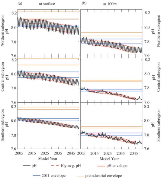
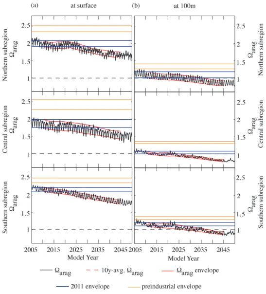
Simulations following the SRES A2 emissions scenario show that increasing atmospheric CO2concentrations cause the pH and arag of the nearshore regions along the US West Coast to move out of their modeled preindustrial and projected present-day variability envelopes before 2050 (Figs. 11 and 12, orange and blue lines). By model year 2011, nearshore waters along the US West Coast have al-ready moved out of the preindustrial envelope. In the north-ern CCS, pH has only recently departed from the preindus-trial variability range due to its large temporal variability (Fig. 11a, upper panel). The fast progression of ocean acidi-fication forces the pH of the northern subregion to move out of its modeled present-day variability envelope by 2045, de-spite the large temporal variability. Surface pH in the central subregion is projected to depart from its present-day enve-lope by 2037 (Fig. 11a, center panel). Surfacearagis pro-jected to move out of its present-day envelope earlier than pH (Fig. 12a). Already by 2030, the northern CCS is projected to be exposed to lower levels of surfacearagthan experienced in 2011 (Fig. 12a, upper panel). Similarly, surfacearag of the central subregion will depart from its present-day enve-lope by 2035 (Fig. 12a, center panel).

By 2023, surface pH and surface arag of the southern subregion are projected to decrease below the range of their relatively small, modeled present-day temporal variability (Figs. 11a and 12a, lower panels). However, these results have to be taken with caution, since our model does not

re-produce the large variability observed in the southern CCS. We therefore expect that pH andaragin the southern sub-region will remain within their variability envelopes longer than projected by the model (see Sect. 3 and Discussion).

At 100 m depth, pH andarag of the northern CCS are projected to depart from their modeled present-day variabil-ity envelopes by 2033, while in the central and southern CCS this transition is projected to take place already a decade ear-lier (Figs. 11b and 12b). In addition, permanent undersatura-tion ofaragat 100 m is projected before 2025 in the central and 2035 in the southern and northern CCS.

In a second simulation under which atmospheric CO2 con-centrations follow the “low-CO2” (B1) emissions scenario, surface pH of the northern subregion is not projected to move out of its present-day envelope before 2050 (see Fig. A2, up-per panel). The projected lower atmospheric CO2 concentra-tions, however, do not affect the timing of transition ofarag in the north (Fig. A2, upper panel), and pH andaragin the central and southern CCS (Figs. A2a and A3a, center and lower panels). This is because their variability range is low, leading to a departure from their variability envelopes before the atmosphericpCO2paths of the two emissions scenarios diverge around 2035 (Fig. S5 in Gruber et al., 2012).

The high spatial variations in the temporal variability within each subregion (especially the northern subregion) leads to a large spatial difference in the timing of the transi-tion outside the variability envelope. Figures 13 and 14 illus-trate the percentage of overlap between the variability range (mean±_{(1 STD}×_{varcf)) of a detrended 10-yr period from}

2005 to 2015 of pH andarag, and the variability range for 10-yr periods of pH and arag for each following decade. The years 2020, 2030 and 2040 are chosen as midpoints for each 10-yr period. Nearshore areas, especially in the northern subregion, retain more than 50 % range overlap until 2030. These areas are exposed to the strongest upwelling and expe-rience the largest range of pH andaragdue to the upwelled cold, DIC- and nutrient-rich water. However, areas in the cen-tral CCS, south of Monterey Bay (36◦48 N, 121◦54 W), are projected to experience pH andaragvalues outside of the present-day envelope by 2030. At 100 m depth, nearshore areas of the central and southern CCS are projected to be exposed to levels outside of the present-day range by 2020, while offshore areas retain some degree of overlap of range until 2030. In the northern subregion, the present-day range of pH andarag in nearshore regions still overlap by about 50 % until 2030.

4.5 Shoaling of the aragonite saturation horizon

(14)

Fig. 11.Simulated time series of monthly mean pH (black) at(a)the surface and(b)100 m depth, for the northern (top panel), central (center panel) and southern (bottom panel) subregions, with the 10-yr running average (red dashed line) for all grid cells of each subregion. The area between the solid lines defines the range of annual variability or envelope (mean±(1 STD×varcf)) of pH for the preindustrial (orange, ∼270 ppm atmosphericpCO₂), 2011 (black,∼395 ppm atmosphericpCO₂) and transient (red) simulations. The envelopes are adjusted with the correction factor varcf(Sect. 2.4).

shows that after reaching the upper 100 m, the shoaling of the aragonite saturation horizon slows down substantially in all subregions. The saturation horizon is highly sensitive to changes in the concentration of CO2₃−where the gradient of CO2₃−concentration with respect to depth is small (Fig. 15). Conversely, when the CO2₃−concentration gradient with re-spect to depth is strong, the saturation horizon is less sensi-tive to small changes of CO2₃−concentration. As a result of these sensitivity differences, the aragonite saturation horizon shoals rapidly from 250 to 100 m because the CO2₃− concen-tration gradient with respect to depth is small in this depth range. Once the saturation horizon enters the upper 100 m, it requires larger changes in CO2₃− to lead to an equivalent shoaling of the aragonite saturation horizon. This explains

why shoaling is initially rapid, and then slows down by about 2025, when the aragonite saturation horizon enters a depth range with larger gradients in CO2₃−concentration.

5 Discussion

(15)

Fig. 12.Simulated time series of monthly meanarag(black) at(a)the surface and(b)100 m depth, for the northern (top panel), central

(center panel) and southern (bottom panel) subregions, with the 10-yr running average (red dashed line) for all grid cells of each subregion. The area between the solid lines defines the range of annual variability or envelope (mean±(1 STD×varcf)) ofaragfor the preindustrial

(orange,∼270 ppm atmosphericpCO2), 2011 (black,∼395 ppm atmosphericpCO2) and transient (red) simulations. The saturation horizon

(arag=1) is indicated by the black dashed line. The envelopes are adjusted with the correction factor varcf(Sect. 2.4).

at a depth of 100–250 m, and in nearshore regions; (2) the model is forced with monthly climatologies of wind and can-not reproduce weather induced, high-frequency events; (3) the riverine input is not explicitly parameterized; (4) conse-quences of global change such as changes in T, winds or precipitation are not taken into account; (5) interannual pro-cesses such as El Ni˜no/La Ni˜na events are not resolved by the model; and (6) ocean acidification-induced changes to important biological processes, such as calcification, photo-synthesis and nitrification are not considered by the NPZD2 ecosystem model.

(16)

Fig. 13. The proportion of overlap in annual pH range (mean±(1 STD×varcf)) of a 10-yr average at present for(a)the

surface and(b)at 100 m depth, compared to 10-yr averages of ev-ery following decade until 2040. The years shown are the midpoints of the 10-yr average. The envelopes are adjusted with the correction factor var_cf(Sect. 2.4).

the central Oregon shelf (∼100 m) during the majority of the upwelling season. The depth bias between the observed and modeled aragonite saturation horizon is expected to decrease with time, because the shoaling of the aragonite saturation horizon is expected to slow down as it approaches shallower depths (see Sect. 4.5).

In our simulations, day-to-day wind variability was not taken into account since the model was forced with a monthly climatology of momentum fluxes from QuickSCAT-based ocean winds. This does not present a large problem in the northern and central subregions where strong seasonal wind patterns prevail (Dorman and Winant, 1995). However, in the southern CCS, synoptic variability dominates (Leinweber et al., 2009; Dorman and Winant, 1995), which is not well captured by our monthly wind climatologies. As a result, the southern subregion is forced with unrealistically smooth wind patterns. Comparison with the SMBO mooring data (Leinweber and Gruber, 2013) underlines this shortcoming of our model for the southern CCS. The model underesti-mates pH variability (1 STD) by a factor of∼_{3.5. This}

im-plies that the projected transition decades would occur about 20 yr later than inferred from our model results. Considering this caveat, the pH of the southern CCS would move out of

Fig. 14. The proportion of overlap in annual arag range (mean±(1 STD×varcf)) of a 10-yr average at present for(a)the

surface and(b)at 100 m depth, compared to 10-yr averages of ev-ery following decade until 2040. The years shown are the midpoints of the 10-yr average. The envelopes are adjusted with the correction factor varcf(Sect. 2.4).

its preindustrial envelope around 2020 and depart from the present-day levels shortly after 2050. The temporal variabil-ity of surfacearagis underestimated in the model by a factor of∼_{7 at the SMBO mooring, implying that the southern}

sub-region will likely not move out of its preindustrial envelope before 2050. The comparison with observational data derived from the recently deployed mooring off Newport, Oregon (Harris et al., 2013, see Sect. 3) and reconstructed pH and aragfromT and O2time series (Alin et al., 2012) indicate that our modeled size of the variability envelopes is in better agreement with the limited available data in the northern and central CCS than they are in the southern subregion. Taking advantage of the fast-growing US carbon mooring network in the future will help to further constrain the model bias and better predict the present-day variability envelope. Forcing the model with wind products at daily or higher temporal res-olution could help to better simulate the observed high tem-poral variability in the winds and sporadic, strong upwelling events that cause extremely low levels of pH andarag.

(17)

Fig. 15. (a)Evolution of the depth of aragonite saturation horizon as a function of time and depth. The depth of the saturation horizon is depicted as a black line. Panel(b)shows the expected shifts in the [CO2₃−] profiles for the years 2005–2050. The black line indicates the depth of the saturation horizon as a function of [CO2₃−] and depth.

modeled in this study, pH andaragmay not be accurately represented in close proximity to the Columbia River mouth, especially during the rainy months (February–June). Other small rivers along the coast can influence DIC and Alk, but their influence is likely small and often limited to infrequent storm events. The surface T andS restoring described in Sect. 2 improves the mean state, but does not capture the nat-ural variability.

Our study accounted for changes of pH and arag due to atmosphericpCO2 increase. However, additional conse-quences of the anthropogenic pCO2 increase through its effects on the Earth’s radiation balance were not taken into account. These include changes in upwelling intensity, strengthened stratification, warming of surface waters, the deepening of the thermocline (King et al., 2011) and thus potential changes in the seasonal cycle. Integrated effects of global change could possibly accelerate the progression of ocean acidification described here. For example, a time series (1982–2008) of upwelling favorable winds and sea surfaceT suggests that a strengthening of large-scale pressure gradient fields led to increased and protracted upwelling in parts of the central CCS (Garc´ıa-Reyes and Largier, 2010), which in turn would lead to lower surface pH andarag, further exacerbat-ing the effects of increasexacerbat-ingpCO2 on the CCS. In addition

to increased aragonite undersaturation, shoaling of low oxy-gen waters further minimizes habitats of sensitive organisms (Bograd et al., 2008; McClatchie et al., 2010). Oxygen de-clines in the CCS result from decreasing concentrations of oxygen in the Equatorial and Eastern Pacific (Stramma et al., 2008, 2010; Bograd et al., 2008). These oxygen declines are thought to be due to increased stratification resulting from global warming (Stramma et al., 2008). As a result of contin-ued global warming and intensified upwelling, hypoxic areas are expected to further expand in the CCS in the future.

The dynamics of the CCS is strongly modified by inter-annual to decadal climate modes such as El Niño/La Niña events or the Pacific Decadal Oscillation, which are not re-solved by our model. The La Niña event in 2010 uplifted the isopycnals in late summer and doubled the period of normal seasonal exposure to undersaturated conditions on the con-tinental shelf off California (Nam et al., 2011). The season of occurrence of La Niña events is variable. It is therefore possible that La Niña amplifies the effect of natural seasonal upwelling, leading to more extreme hypoxic and aragonite undersaturated conditions. As a result, variability envelopes would be widened and the transitions toward the conditions outside these envelopes would be delayed, while seasonal aragonite undersaturation would occur earlier.

Ocean acidification may trigger several physiological re-sponses in organisms, some of which may lead to significant changes in the DIC and Alk concentrations. However, none of these potential responses are represented in our simple NPZD2 ecosystem model. Ongoing research suggests that several biological processes can be affected by ocean acid-ification (reviewed in e.g., Doney et al. 2009) with calcifi-cation likely being the most relevant. Coccolithophores as the dominant calcifiers show a wide range of responses in their calcification rates to ocean acidification (e.g., Riebesell et al., 2000; Langer et al., 2006; Iglesias-Rodriguez et al., 2008), with possible effects on the vertical distribution of Alk (Ilyina et al., 2009). Here, calcium carbonate formation was kept at a fixed rate, introducing additional uncertainty to the study. But given the limited importance of calcifica-tion in controlling pH andaragin the CCS, we consider the potential impact of changes in calcification on our results to be relatively limited.

(18)

6 Conclusions

This study gives new insights into the spatial and temporal dynamics of pH andaragalong the US West Coast. It further enables us to relate the present-day high spatial and tempo-ral variability of pH andaragto their modeled preindustrial and projected future ranges of pH andarag. While a few nearshore areas of the central and northern subregions are presently exposed to temporary undersaturation, our results also highlight the fact that the nearshore ecosystems along the US West Coast are already exposed to pH andarag lev-els outside of the modeled preindustrial variability envelope. Additionally, as early as ∼_{2040, surface pH and} arag of the nearshore US West Coast are projected to move out of the modeled present-day variability envelope under increas-ing atmospheric CO2 concentrations as projected from the IPCC SRES A2-Scenario.

The combination of naturally high DIC and the oceanic uptake of anthropogenic CO2 drives the CCS toward un-dersaturation faster than other coastal areas (Blackford and Gilbert, 2007) and on a similar timescale as the Arctic and Southern oceans (Gruber et al., 2012). Despite the high an-nual variability, the absolute decrease of pH andaragis fast and significant enough to cause a departure from its present-day range by 2040. We conclude that these types of changes put the CCS particularly at risk to the effects of ocean acidifi-cation. Given the imminent departure from preindustrial en-velopes, we speculate that these effects may already be well underway.

Marine ecosystems of the CCS are exposed to a variety of stress factors, many of which are projected to increase in the future. Along with the developing problem of ocean acid-ification, organisms will have to deal with warming of the waters, an expansion of hypoxic areas and changes of the vertical structure of the water column (Gruber, 2011; Doney et al., 2012). Furthermore, non-climate change-related im-pacts, such as pollution, eutrophication and overfishing fur-ther increase the vulnerability of the CCS ecosystems. To-gether, these stressors compound the challenges that many organisms of the CCS will face in the coming decades and will necessitate rapid migration, acclimation or adaptation in order to cope with these changing environmental conditions.

Appendix A

Description of the carbon biogeochemistry module

The carbon biogeochemistry module adds the three new state variables DIC, Alk and CaCO3(DCaCO3) to the model. The

conservation equation for any tracer concentrationBis given by

∂B

∂t = ∇ ·| K{z∇B} diffusion

− u· ∇hB | {z } horiz. advection

−

w+wsink _∂B

∂z

| {z }

vert. advection & sinking (A1)

+ J (B) | {z } source minus sink term

,

whereKis the eddy kinematic diffusivity tensor,∇_{is the 3-D}

gradient,∇_h_{is the horizontal gradient,}u_{denotes the}

horizon-tal andwthe vertical velocities of the fluid, andwsinkis the vertical sinking rate of all particulate pools, except zooplank-ton (see Table A1).J (B)denotes the source minus sink term for each tracer, which is described in detail for DIC, Alk and DCaCO₃ in the following. The remaining source minus sink terms for the other model state variables are defined in Gru-ber et al. (2006).

The sources and sinks of DIC include net community pro-duction, gas exchange, and CaCO3 formation and dissolu-tion:

J (DIC)= −µmax_P (T , I )·_{γ (NO}−

3,NH

+

4)·P·rC : N

| {z }

net primary production

(A2)

−k_CaCOform

3·µ

max

P (T , I )·γ (NO

−

3,NH

+

4)·P·rC : N

| {z }

CaCO3formation +k_Dremin

S DS·rC : N+k

remin

DL DL·rC : N

| {z }

detritus remineralization

+ ηmetab_Z Z·rC : N

| {z }

zooplankton respiration

+kdiss_CaCO

3DCaCO3

| {z }

dissolution

+ k_Sremin

D SD·rC : N

| {z }

sediment remineralization atk=1

+k_Sdiss

CaCO3SCaCO3·rC : N

| {z }

sediment dissolution atk=1

+ JGas |{z} gas exchange

.

This equation follows the nomenclature used in Gruber et al. (2006). Symbols with parentheses, such asµmax_P (T,I) rep-resent functions of the respective variables.JGasis the gas exchange flux described below (Eq. A3). The state variable associated with the function/parameter is denoted in the sub-script, while the corresponding process is given in the su-perscript. The variables in the equation denote the follow-ing: I and T are light and temperature, respectively, P is the phytoplankton pool,Zis the zooplankton pool,DSis the small detritus pool,DLis the large detritus pool,DCaCO3 is

the CaCO3pool in the water column,SDis the nitrogen and SCaCO3 is the CaCO3pool in the sediment. All relevant

pa-rameters are described in Table A1. The carbon fluxes are tied to those of nitrogen with a fixed stoichiometric ratiorC : N of 106:_{16 (Redfield et al., 1963).}

(19)

Table A1. Summary of the definitions, symbols, values and units of the parameters used in the carbon module of the ecological-biogeochemical model.

Parameter Symbol Value Units

Carbon to nitrogen ratio of organic matter rC : N 6.25 –

Remineralization and respiration parameters

Remineralization rate ofD_S k_Dremin

S 0.03 day

−1

Remineralization rate ofDL k_Dremin_L 0.01 day−1

Zooplankton basal metabolism rate ηmetab_Z 0.1 day−1

CaCO3formation and dissolution parameters

CaCO3fraction of net primary production kCaCOform3 0.07 –

CaCO3dissolution rate k_CaCOdiss ₃ 0.0057 day−1

Sediment parameters

Sediment remineralization of organic matter k_Sremin

D 0.003 day

−1

Sediment dissolution of CaCO₃ k_Sdiss

CaCO3 0.002 day

−1

Sinking parameters

Sinking velocity ofP wsink_P 0.5 m day−1

Sinking velocity ofDS wsink_D_S 1.0 m day−1

Sinking velocity ofDL wsink_D_L 10.0 m day−1

Sinking velocity ofDCaCO3 w

sink

D_CaCO3 20.0 m day

−1

whether phytoplankton (P) take up NH+₄ or NO−₃, nitrogen adds to either the regenerated or the new production flux, re-spectively. The modeled phytoplankton growth is limited by temperature (T), light (I) and the concentrations of NO−₃ and NH+₄.µmax_P (T,I) is the temperature-dependent, light-limited growth rate ofP under nutrient replete condition.γ(NO−₃, NH+₄) is a non-dimensional nutrient limitation factor, with a stronger limitation for nitrate than ammonium, taking into account thatP take up NH+₄ preferentially over NO−₃ and that the presence of ammonium inhibits the uptake of nitrate byP. For a more detailed description of these limitation fac-tors the reader is referred to Gruber et al. (2006).

Formation ofDCaCO₃ also decreases the DIC pool and is parameterized as 7 % of the net primary production, such that for each mole of organic carbon formed by net primary pro-duction, 0.07 mol ofDCaCO₃ are formed.DCaCO₃ dissolves at a fixed first order rate of 0.0057 day−1_{. This process releases} CO2₃−, and thus adds to the DIC pool. The full source minus sink equation forDCaCO3 is described below (Eq. A6).

Zooplankton (Z) are parameterized with one size class (mesozooplankton). The Z respiration from basal metabolism and remineralization processes increases the total DIC pool. Large detritus (DL) is remineralized at a rate of 0.01 m day−1 and small detritus (DS) at a rate of 0.03 m day−1. The different sinking speeds and remineraliza-tion rates of small and large detritus result in a large differ-ence of the remineralization length scales of 30 m forDSand

1000 m forDL. As a consequence,DLis rapidly transported to depths below the euphotic zone, whileDS is subjected to offshore transport and is absent in the ocean interior (Gruber et al., 2006).

The sediment is parameterized as a simple one layer model added to the bottom layer (k=_{1) of the model. The}

sedi-ment is represented by the state variablesSD (mmol N m−2) andSCaCO3 (mmol C m

−2_{). Once organic matter and CaCO3} arrive at the sediment surface they are accumulated in the sediment layer. The accumulated organic matter and CaCO3 are subjected to first-order decomposition reactions that re-lease dissolved material into the deepest model layerk=₁

and thus back into the water column.

Gas exchange is parameterized following Wanninkhof (1992):

JGas=_COsol

2 ·k·(pCO air 2 −pCO

ocean

2 ), (A3)

where

(20)

Table A2.Evaluation of model with regard to its spatial variability: Shown are the normalized model standard deviation (norm. STD.), the correlation coefficient and bias of observed and modeled pH,

arag, Alkalinity, DIC, Temperature and Salinity. A five-year aver-age of modeled parameters over May and June (2006–2010) are compared to observations sampled between May and June 2007 (Feely et al., 2008), for all sampled locations (CCS), the subregions north, central, southern, for 0–100 m, 100–250 m and 500–5000 m. The modeled standard deviations were normalized relative to the observed standard deviations from Feely et al. (2008). Specified units correspond only to the absolute bias.

Property Location norm. Correlation Absolute

STD coefficient bias

CCS 0.74 0.89 −0.06

northern 0.73 0.91 −0.07

central 0.76 0.89 −0.05

pH southern 0.71 0.89 −0.07

0–100 m 0.58 0.74 −0.04

100–250 m 0.33 0.43 −0.10

250–4500 m 0.91 0.68 −0.09

CCS 0.83 0.89 −0.11

northern 0.79 0.91 −0.11

central 0.87 0.89 −0.09

Aragonite southern 0.82 0.88 −0.12

0–100 m 0.64 0.74 −0.08

100–250 m 0.52 0.58 −0.15

250–4500 m 1.37 0.83 −0.11

CCS 0.88 0.92 −6

northern 0.77 0.93 −20

central 0.95 0.92 −4

Alkalinity southern 1.04 0.94 −1

(µmol kg−1) 0–100 m 0.40 0.79 −6

100–250 m 0.63 0.68 −6

250–4500 m 0.99 0.99 −8

CCS 0.87 0.92 14

northern 0.79 0.93 3

central 0.91 0.92 12

DIC southern 0.91 0.93 21

(µmol kg−1) 0–100 m 0.56 0.77 10

100–250 m 0.57 0.69 22

250–4500 m 1.21 0.98 13

CCS 1.15 0.95 −0.31

northern 1.05 0.95 −0.03

central 1.15 0.93 −0.31

Temperature southern 1.18 0.95 −0.47

(C◦) 0–100 m 0.97 0.85 −0.90

100–250 m 1.13 0.88 0.40

250–4500 m 0.87 0.99 0.44

CCS 0.78 0.86 0.18

northern 0.69 0.88 0.004

central 0.91 0.83 0.20

Salinity southern 1.14 0.86 0.26

(PSU) 0–100 m 0.50 0.87 0.21

100–250 m 0.88 0.71 0.22

250–4500 m 1.08 0.90 0.04

Fig. A1.Seasonal cycle of(a)surface chlorophyllaand(b) nitri-fication at 100 m, in the nearshore 50 km. The lines represent the mean and the shaded area the spatial variability (±1 STD) for each month, for the northern (blue), central (orange) and southern (red) subregions. The shaded area depicts the first six months of the fol-lowing annual cycle.

chemistry routines3. The routines used the carbonic acid dis-sociation constants of Mehrbach et al. (1973), as refit by Dickson and Millero (1987) and Dickson (1990). The pres-sure effect on the solubility was estimated from the equation of Mucci (1983), including the adjustments to the constants recommended by Millero (1995).kis the gas transfer coef-ficient given by equation three in Wanninkhof (1992), which is dependent on the square of the instantaneous wind speed (u) and the temperature dependent Schmidt number (Sc).

Alk increases due to the removal of NO−₃ (new production) and dissolution of CaCO3and decreases due to the formation of NO−₃ (nitrification) and formation of CaCO3:

J (Alk)= +2·k_CaCOdiss

3DCaCO3

| {z }

dissolution

(A5)

+µmax_P (T , I )·γ (NO−₃)·P·rC : N

| {z }

new production

+ 2·k_Sdiss

CaCO3SCaCO3

| {z }

sediment dissolution atk=1

−2·k_CaCOform

3·µ

max

P (T , I )·γ (NO

−

3,NH

+

4)·P·rC : N

| {z }

CaCO3formation −knitr(I )·_NH+

4

| {z }

nitrification .

(21)

Fig. A2.Simulated time series of monthly mean surface pH for the two employed IPCC-SRES scenarios A2 (red) and B1 (blue), for the northern (top panel), central (center panel) and southern (bot-tom panel) subregions, with the 10-yr running average (dashed red and blue lines) of the mean for all grid cells of each subregion. The area between the solid lines defines the range of annual variability or envelope (mean±1 STD) of pH for 2011 (black,∼395 ppm at-mosphericpCO2) and the transient simulations following the A2

(red) and B2 (blue) emissions scenarios. The results are based on simulations with the 15-km resolution set-up.

Nitrification is light-limited (I) and parameterized at a rate of 0.05 day−1 (see Gruber et al., 2006). CaCO3 formation and dissolution processes change Alk twice as much as DIC. This can be explained from the definition of alkalin-ity (Dickson, 1981) where the addition (removal) of 1 mol of CO2₃−results in a 2 mol change in Alk.

The concentration of CaCO3(mmol C m−3_{) is dependent} on net primary production and dissolution:

J (DCaCO3)=k

form CaCO3·µ

max

P (T , I )·γ (NO

−

3,NH

+

4)·P ·rC : N

| {z }

CaCO3formation −kdiss_CaCO

3DCaCO3

| {z }

dissolution

. (A6)

CaCO3increases by 0.07 mol (k_CaCOform

3) for each mole of

or-ganic carbon produced by net primary production and it dis-solves at a fixed rate of 0.0057 day−1 (kdiss_CaCO

3) in the water

column and at 0.002 day−1(kdiss_S

CaCO3) in the sediment.

Fig. A3.Simulated time series of monthly mean surfacearagfor

the two employed IPCC-SRES scenarios A2 (red) and B1 (blue), for the northern (top panel), central (center panel) and southern (bottom panel) subregions, with the 10-yr running average (dashed red and blue lines) of the mean for all grid cells of each subregion. The area between the solid lines defines the range of annual variability or envelope (mean±1 STD) ofaragfor 2011 (black,∼395 ppm atmosphericpCO₂) and the transient simulations following the A2 (red) and B2 (blue) emissions scenarios. The results are based on simulations with the 15-km resolution set-up.

Acknowledgements. We are grateful to Damian Loher for his support with the model simulations. We thank Thomas Fr¨olicher, Fortunat Joos and Marco Steinacher who kindly provided us with results from their NCAR CSM 1.4-carbon model simulations. We would also like to thank Simone Alin and Katherine Harris for the observational data and Kay Steinkamp, Mark Payne and Diego Santaren for beneficial discussions and statistical support. C. H. was supported by the European Project of Ocean Acidi-fication (EPOCA), which received funding from the European Community’s Seventh Framework Programme (FP7/2007–2013) under grant agreement no. 211384. EPOCA is endorsed by the international programs Integrated Marine Biogeochemistry and Ecosystem Research (IMBER), Land-Ocean Interactions in the Coastal Zone (LOICZ), and Surface Ocean Lower Atmosphere Study (SOLAS). C. H., M. V., Z. L., A. M. P. M. and N. G. also acknowledge support by ETH Zurich. S. D. acknowledges support from NASA-NNX11AF55G.