Statistical dependence of auroral ionospheric currents on solar wind and geomagnetic parameters from 5 years of CHAMP satellite data

(1)

www.ann-geophys.net/27/1005/2009/

Annales

Geophysicae

Statistical dependence of auroral ionospheric currents on solar wind

and geomagnetic parameters from 5 years of CHAMP satellite data

L. Juusola1, K. Kauristie1, O. Amm1, and P. Ritter2

1_{Finnish Meteorological Institute, P.O. Box 503, 00101, Finland}

2_{Helmholtz-Zentrum Potsdam, Deutsches GeoForschungsZentrum (GFZ), Telegrafenberg, 14473 Potsdam, Germany}

Received: 2 October 2008 – Revised: 13 January 2009 – Accepted: 4 February 2009 – Published: 2 March 2009

Abstract. The effects of the solar wind dynamic

pres-sure (P), thezcomponent of the solar wind magnetic field (Bz), the merging electric field (Em), season and theKp

in-dex on R1 and R2 field-aligned currents are studied statis-tically using magnetic field data from the CHAMP satellite during 2001–2005. The ionospheric and field-aligned cur-rents are determined from the magnetic field data by the recently developed 1-D Spherical Elementary Current Sys-tem (SECS) method. During southward IMF, increasing |Bz| is observed to clearly increase the total field-aligned

current, while during northward IMF, the amount of field-aligned current remains fairly constant regardless of _|Bz|.

The dependence of the field-aligned current onBzis given by

|Ir[MA]|=0.054·Bz[nT]2−0.34·Bz[nT]+2.4. With

increas-ing P, the intensity of the field-aligned current is also found to increase according to_|Ir[MA]|=0.62·P[nPa]+1.6,

and the auroral oval is observed to move equatorward. Increasing Em produces similar behaviour, described by

|Ir[MA]|=1.41·Em[mV/m]+1.4. While the absolute

inten-sity of the ionospheric current is stronger during negative than during positiveBz, the relative change in the intensity

of the currents produced by a more intense solar wind dy-namic pressure is observed to be approximately the same re-gardless of theBz direction. IncreasingKp from 0 to≥5

widens the auroral oval and moves it equatorward from be-tween 66◦_–74◦_{AACGM latitude to 59}◦_–71◦ _{latitude. The}

total field aligned current as a function of Kp is given by

|Ir[MA]|=1.1·Kp+0.6. In agreement with previous studies,

total field-aligned current in the summer is found to be 1.4 times stronger than in the winter.

Keywords. Ionosphere (Auroral ionosphere; Electric fields

and currents; Ionosphere-magnetosphere interactions)

Correspondence to:L. Juusola

([email protected])

1 Introduction

A significant part of the solar wind energy that penetrates the Earth’s magnetosphere is dissipated in the polar ionospheres. The most important dissipation mechanisms are Ohmic Joule heating and particle precipitation in the auroral regions (e.g., Brekke, 1997). Therefore, it is important to understand the effect the different conditions of the solar wind have on the large-scale ionospheric currents. The amount of energy con-sumed by Joule heating can be estimated statistically from ground-based magnetic field variations. Since Joule heat-ing is related to Pedersen currents, while ground-based varia-tions are mostly produced by Hall currents, understanding of how the Hall currents can describe the Pedersen currents is also needed. Satellite magnetic field measurements are well suited to studying the problem, since, unlike from ground-based magnetic field measurements, all three components of the ionospheric current density can be determined from them (Fukushima, 1976).

The main driver of ionospheric activity is the solar wind-magnetosphere-ionosphere interaction. The solar wind en-ergy enters the magnetosphere by magnetic reconnection and viscous interaction (Dungey, 1961; Axford and Hines, 1961). The electric field (E) generated by the solar wind as it flows across the open magnetic field lines of the polar cap (Bgeo)

maps from the magnetosphere to the ionosphere, where it drives electric currents according to Ohm’s law:

J ₌JP +JH =6PE−6H

E_×Bgeo

Bgeo

, (1)

where JP, JH, 6P and 6H are the Pedersen and Hall

current densities and conductances, respectively. The field-aligned current density is related to the divergence of the hor-izontal current density

j_|| _{= ∇ ·}J. (2)

(2)

region 1 (R1) and region 2 (R2) systems. The poleward R1 currents flow into the ionosphere on the dawnside and out of the ionosphere on the duskside, whereas the equatorward R2 currents have an opposite polarity at a given local time (Iijima and Potemra, 1976). While statistically the currents are strongest in the dawn and dusk sectors, the most intense currents can be found on the nightside during substorms (e.g., Kamide and Baumjohann, 1993). With increasing activity, the current system intensifies and expands to lower latitudes. The horizontal ionospheric currents consist of Pedersen cur-rents that mainly connect the regions of upward and down-ward field-aligned current, and Hall currents that flow an-tiparallel to the plasma convection. The eastward and west-ward electrojets in the dusk and dawn sectors of the auroral oval, and the Harang discontinuity on the nightside, are the predominant features of this component.

Several factors can contribute to interhemispheric asym-metry of the currents. Local anomalies in the geomagnetic field are one source. Seasonal variations in local solar ra-diation affect the ionospheric conductivity and thereby the intensity of the currents. Due to the effect of the dipole tilt on the magnetospheric configuration, the dayside field-aligned currents move poleward in the summer hemisphere and equatorward in the winter hemisphere, while the night-side field-aligned currents have the opposite seasonal de-pendence (Ohtani et al., 2005). According to the direction of the interplanetary magnetic field (IMF), reconnection on the dayside magnetopause can result in either symmetric or asymmetric convection patterns in the two hemispheres. When the IMF is southward (Bz<0), plasma flows

antisun-ward across the polar cap and sunantisun-ward in the auroral oval, forming a two-cell convection pattern. ForBy≈0, the pattern

is symmetric. ForBy<0, the dawn cell becomes rounder and

the dusk cell crescent-shaped, whereas forBy>0, the dusk

cell becomes rounder and the dawn cell crescent-shaped in the Northern Hemisphere. In the Southern Hemisphere, for a given sign ofBy, the behaviour of the cells is reversed. When

IMF is northward (Bz>0), the convection patterns are more

complex, for instance forming multiple cells (e.g., Schunk and Nagy, 2000). During strongly positiveBz, the

configura-tions in the two hemispheres may be very different (Lu et al., 1994).

In a superposed epoch analysis, Ritter et al. (2004) showed the merging electric fieldEm(Kan and Lee, 1979) to be

suit-able for describing the geoeffectiveness of the solar wind-magnetosphere coupling.Emis defined as

Em=V

q

B_y2₊B_z2sin2(θ/2), (3) whereV is the solar wind speed,By andBzare the GSMy

andzcomponents of the IMF, andθ₌arctan(By/Bz)is the

IMF clock angle.

The intensity of the field-aligned currents that couple mag-netospheric processes to the high-latitude ionosphere is af-fected by the ionospheric conductivity. In the ionospheric

E-layer, ionisation of the neutral particles are caused by so-lar extreme ultra-violet (EUV) radiation and collisions with precipitating, energetic particles associated with the field-aligned currents (e.g., Schunk and Nagy, 2000). The dif-ference in the solar radiation between the winter and the summer hemispheres affects mostly conductivity on the day-side. Also particle precipitation varies with season: Using global auroral images from the Polar ultraviolet imager in the Northern Hemisphere during the winter 1996 and the sum-mer 1997, Liou et al. (2001) have shown that nightside au-roral precipitation power is suppressed and dayside power enhanced in the summer. Using a magnetohydrodynamic (MHD) simulation, Ridley (2007) demonstrated that if only the solar driven conductance changes were taken into ac-count, the ratio between the maximum summer field-aligned current and maximum winter field-aligned current was_∼4. Including a seasonally dependent auroral precipitation to in-crease the auroral conductance in the winter hemisphere re-duced the ratio to 1.6.

Several studies have investigated the seasonal dependence of large-scale field-aligned currents using satellite-based vec-tor magnetic field measurements. Weimer (2001) observed the field-aligned current intensities to be much stronger dur-ing summer than winter. Accorddur-ing to Papitashvili et al. (2002), the ratio of total summer/winter field-aligned current is 1.35 and, according to Christiansen et al. (2002), 1.5–1.8. Fujii et al. (1981) and Wang et al. (2005) found the seasonal effect to be confined mainly on the dayside.

The effect of the solar wind dynamic pressure on the ionospheric dynamics has been studied by Palmroth et al. (2004). They inferred from a statistical superposed epoch analysis that during steady southward IMF, solar wind pres-sure pulses, as observed by ACE, increased theAE index. The AE index is often used as a proxy for Joule heating. During steady northward IMF, such a response was not ob-served. On the other hand, using a global MHD simulation, they found that Joule heating was positively correlated with the solar wind dynamic pressure both during southward and northward IMF. According to the simulation, increasing dy-namic pressure increases field-aligned current, which then increases Joule heating.

Using particle precipitation data from the Defense Meteo-rological Satellite Program (DMSP) spacecraft, Boudouridis et al. (2003) studied the effect of large solar wind dynamic pressure increases on the location, size and intensity of the auroral oval during three events with various IMF orienta-tion. All three events showed a change of the auroral oval location, size, and intensity in response to the pressure pulse. Most prominent changes, an increase of the auroral zone width and a decrease of the polar cap size, were observed during steady southward IMF. When the IMF turned simul-taneous northward, and when it was nearly zero before the pressure enhancement, smaller responses were perceived.

In this study, we analyse statistically the effect of theKp

(3)

dynamic pressure (P), and the merging electric field (Em)

on the large-scale ionospheric currents using magnetic field measurements from the CHAMP satellite. All three compo-nents of the ionospheric current density are derived from the magnetic field data using the relatively new 1-D Spherical Elementary Current System (SECS) technique (Vanham¨aki et al., 2003; Juusola et al., 2006). Especially, we are inter-ested in the differences produced by changes inBz,P and

Em. We start by describing how the statistical current

distri-butions have been derived from the magnetic data (Sect. 2). Section 3 contains an overview of the data and of the differ-ences between the Northern and the Southern Hemispheres. In Sect. 4, the data are binned with respect to activity, in Sect. 5, with respect to season, in Sect. 6, with respect to BzandP, and in Sect. 7, with respect toEm. The last two

sections contain discussion and a summary.

2 Data processing

In this study, the variation magnetic field measurements from the CHAMP (CHAllenging Minisatellite Payload) satellite during the years 2001–2005 have been used. On 15 July 2000, the CHAMP satellite was launched into an almost circular, near polar (i₌87◦_{) orbit with an initial altitude of}

454 km, but due to atmospheric drag, the altitude had de-creased to _∼350 km by the end of 2005. CHAMP has a period of _∼1.5 h, resulting in over 15 revolutions per day, and all local time sectors are covered in 131 days. The vec-tor magnetic field is measured by the fluxgate magnetometer on board. We have used the 1 Hz data, which corresponds to_∼7.5 km distance between successive measurement. The magnetic field (Br,Bθ,Bφ) was obtained by subtracting from

the measurements the CO2 main field model (Holme et al., 2003), employed up to degree and order 14, and the ring cur-rent effect (Dst-correction) using the external set of

coeffi-cients of the same model.

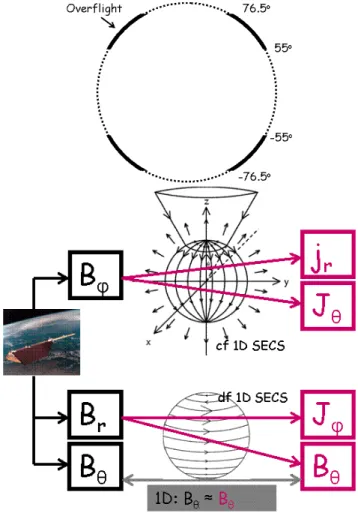
For the analysis, the data were first converted from ge-ographic coordinates (GEO) to geomagnetic dipole coordi-nates (MAG), and each orbit was divided into four overflights between 55◦_–76.5◦_{northern and southern MAG latitude, as}

illustrated in the top panel of Fig. 1. During each overflight, the current distribution was assumed to be stationary, and 1-D (independent of longitude in some coordinate system), which is a reasonable assumption for electrojet dominated events. The full ionospheric and field-aligned current den-sity for each the overflight was then computed using the 1-D SECS technique.

The determination of the ionospheric current density (jr[A/km2],Jθ[A/km],Jφ[A/km]) from the magnetic field

measured by the satellite (Br,Bθ,Bφ) using the 1-D SECS

method is illustrated in the bottom panel of Fig. 1: The hor-izontal ionospheric current density at the altitude of 100 km can be divided into curl-free (cf) and divergence-free (df) parts. For uniform conductances,Jcf(θ, φ)would then

cor-Fig. 1. Left: Division of one orbit into four overflights between 55◦_...₇₆_.₅◦_and₋₇₆_.₅₅◦_...₋₅₅◦_{MAG latitude. Right:}

Determi-nation of the ionospheric current density (jr,Jθ,Jφ) from the

mag-netic field measured by a satellite (Br,Bθ,Bφ) using the 1-D SECS

method (picture of CHAMP: courtesy of http://www.gfz-potsdam. de/pb1/op/champ/).

respond to Pedersen currents and Jdf(θ, φ) to Hall

cur-rents. Field-aligned currentsjr(r, θ, φ)are associated with

the divergence of the curl-free currents, and are assumed to flow radially. In a 1-D case, that is, when the cur-rent distribution is independent of φ, Jcf(θ )=Jθ(θ )θˆ and

Jdf(θ )=Jφ(θ )φˆ. The magnetic field caused by jr(r, θ )

and Jθ(θ ) is B=Bφ(r, θ )φˆ and the magnetic field caused

by Jφ(θ ) is B=Br(r, θ )rˆ+Bθ(r, θ )θˆ. Jθ andjr can now

be computed from Bφ using the curl-free 1-D SECSs and

similarly, Jφ could be determined from Br and Bθ using

the divergence-free 1-D SECSs. Instead, however, we have only usedBr and also computed Bθ from it. By

compar-ing the measured and computedBθ, we could then determine

(4)

55 60 65 70 −100

−50 0

Br

(nT)

2001−11−20 03:58:41 ... 2001−11−20 04:04:41 UT

1D SECS CHAMP

55 60 65 70 −100

−50 0

Bθ

(nT)

error = 23 %

55 60 65 70 −300

−200 −100 0

1D latitude (79o,−103o)

Bφ

(nT)

55 60 65 70 −0.6

−0.4 −0.2 0 0.2

jr

(A/km

2)

06:56:13 ... 06:00:54 MLT

55 60 65 70 0

100 200

Jθ

(A/km)

55 60 65 70 −400

−200 0

1D latitude (79o,−103o)

Jφ

(A/km)

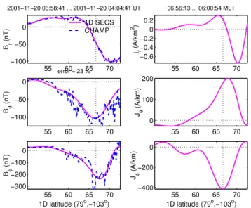
Fig. 2. Magnetic field measured by CHAMP and the ionospheric current density computed using the 1-D SECS method as a func-tion of 1-D latitude on 20 Nov 2001 between 03:59–04:04 UT.Br,

Bθ, andJφare determined fromBr andBφ,jr, andJθ fromBφ.

The north pole of the 1-D coordinate system is located at 79◦GEO lat and -103◦ lon. In these coordinates, Jcf(θ ) = Jθ(θ )θˆ and J_df(θ )=Jφ(θ )φˆ.

In order to optimally apply the 1-D SECS technique, the best 1-D coordinate system was determined for each over-flight. The 1-D coordinate system is a spherical coordinates system similar to MAG, but its pole is displaced from the MAG pole. The optimal displacement for each overflight was determined by minimizing the difference between the mea-sured and computedBθ. If such a coordinate system could be

found, where the difference was small enough, the overflight was termed 1-D (see Juusola et al., 2007, for more details). An example of the application of the 1-D SECS method for one overflight is shown in Fig. 2.

After the calculation of the current density, the overflights that did not fulfil the 1-D condition were rejected. 44265 out of the total of 113 700 overflights (39%) were categorized as being 1-D. For the statistics, the current densities at 100 km altitude were converted from the 1-D coordinates to Alti-tude Adjusted Corrected Geomagnetic (AACGM; Gustafs-son et al., 1992) coordinates and divided into cells of 1◦ _in

AACGM latitude and 0.5 h in Magnetic Local Time (MLT). By experimenting, cells with less than 500 data points were rejected, and for the others, the average was computed. This was done separately forJcf,θ,Jcf,φ,Jdf,θ,Jdf,φ, andjr. In

Fig. 3, for instance, the rejected data cells have been plotted in white.

To be able to compare the location and the width of the auroral oval in different bins, a simple estimate for the pole-ward and equatorpole-ward boundaries of the oval was needed. This was achived by first averaging the absolute value of the

field-aligned current in each cell (_|Ir(lat,MLT)|[A]) over the

MLT sectors 04:00–06:00 and 18:00–20:00, where the statis-tics were most reliable, and then determining the oval bound-aries from the condition that 15.9% of|Ir(lat)|lay

equator-ward of the equatorequator-ward boundary of the oval and, similarly, that 15.9% of_|Ir(lat)|lay poleward of the poleward

bound-ary of the oval. For a normal or Gaussian distribution, 68.3% of the values lie within one standard deviation from the mean, and, hence, 2_×15.9% of the values lie outside. The resulting oval boundaries have been marked in Fig. 3 by black arcs.

The data have been binned with respect to season, theKp

index, solar wind dynamic pressure, IMFBz, and the

merg-ing electric field. 1-min resolution solar wind data propa-gated to the magnetopause at_∼10REfrom the GSFC/SPDF

OMNIWeb interface at http://omniweb.gsfc.nasa.gov was used for this purpose.

The regions of missing data vary in size and location tween bins. This made it more difficult to compare data be-tween any bins, and therefore, we have only calculated Ir

from those_|lat_|and MLT regions where all bins that were being compared had data. The missing data regions are still slightly different, for instance, for the season- andP-bins. These differences may make it more difficult to compare some of the results, for instance the total field-aligned cur-rent, but the other option of equalizing all missing data re-gions would, on the other hand, have resulted in poorer statis-tics. Mainly, however, the regions over which the total field-aligned current was integrated were similar to that shown in Fig. 3.

3 Ionospheric currents in the Northern and in the

Southern Hemispheres

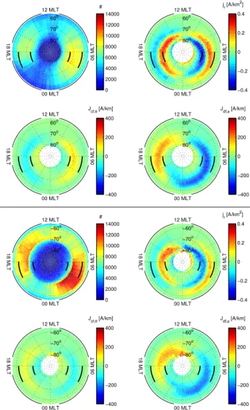
Averaged over long time-sequences, the large-scale iono-spheric currents in the Northern and in the Southern Hemi-spheres are expected to mostly mirror each other (e.g., Schunk and Nagy, 2000). Some differences arise due to the differences in the geomagnetic field between the hemi-spheres, but these effects can mostly be corrected by the use of the AACGM coordinates. In order to observe any remaining effects, Fig. 3 shows the ionospheric currents in the Northern (top) and in the Southern Hemispheres (bot-tom), constructed from all our data during 2001–2005, as described in the previous section, with Kp<6. Averaging

over such a long time sequence should smooth out any dif-ferences produced by short-period effects, leaving only the approximately constant ones.

(5)

0 2000 4000 6000 8000 10000 12000 14000 80o 70o 60o 00 MLT 06 MLT 12 MLT 18 MLT # −0.4 −0.2 0 0.2 0.4 80o 70o 60o 00 MLT 06 MLT 12 MLT 18 MLT j r [A/km

2_] −400 −200 0 200 400 80o 70o 60o 00 MLT 06 MLT 12 MLT 18 MLT J cf,θ [A/km]

−400 −200 0 200 400 80o 70o 60o 00 MLT 06 MLT 12 MLT 18 MLT J df,φ [A/km]

0 2000 4000 6000 8000 10000 12000 14000 −80o −70o −60o 00 MLT 06 MLT 12 MLT 18 MLT # −0.4 −0.2 0 0.2 0.4 −80o −70o −60o 00 MLT 06 MLT 12 MLT 18 MLT j r [A/km

2_] −400 −200 0 200 400 −80o −70o −60o 00 MLT 06 MLT 12 MLT 18 MLT

J_cf,θ [A/km]

−400 −200 0 200 400 −80o −70o −60o 00 MLT 06 MLT 12 MLT 18 MLT

J_df,φ [A/km]

Fig. 3.Ionospheric current density in the northern (top) and in the Southern Hemisphere (bottom): Data point distribution (#), field-aligned current density (jr, positive up),θcomponent of the

curl-free current density (Jcf,θ, north-south component, positive

equa-torward in the Northern Hemisphere and poleward in the Southern Hemisphere), andφcomponent of the divergence-free current den-sity (Jdf,φ, east-west component, positive eastward). The black

arcs denote the poleward and equatorward boundaries of the auroral oval as defined in Sect. 2.

divergence-free current density (east-west component, posi-tive eastward). Due to the 1-D condition, which favors elec-trojet dominated cases, most data points were located in the dawn and dusk sectors of the oval.

In both hemispheres,jr displays the two co-centric rings

of R1 and R2 current with the amplitude of the poleward R1 current ring stronger than that of the equatorward R2 current ring. On the dawnside, Jcf,θ shows that part of the

down-ward R1 current heads equatordown-ward todown-wards the updown-ward R2

0 2000 4000 6000 8000 10000 12000 14000 80o 70o 60o 00 MLT 06 MLT 12 MLT 18 MLT # −0.4 −0.2 0 0.2 0.4 80o 70o 60o 00 MLT 06 MLT 12 MLT 18 MLT j r [A/km

−400 −200 0 200 400 80o 70o 60o 00 MLT 06 MLT 12 MLT 18 MLT J cf,φ [A/km]

−400 −200 0 200 400 80o 70o 60o 00 MLT 06 MLT 12 MLT 18 MLT J df,θ [A/km]

Fig. 4.Combined data from both hemispheres.Jcf,φandJdf,θ are

also shown in addition toJ_cf,θandJ_df,φ.

current, while the rest flows poleward towards the upward R1 current on the dusk side. On the duskside, the downward R2 current flows towards the upward R1 current. The antisun-ward electrojets in the dawn and dusk sectors of the auroral oval and the sunward return current across the polar cap are prominent inJdf,φ. On the nightside, where the two

oppo-sitely directed electrojets overlap, the Harang discontinuity is formed.

The black arcs in the figure denote the poleward and equa-torward boundaries of the auroral oval, as defined in Sect. 2, and lie at 62◦_{and 73}◦_{latitude in the Northern Hemisphere}

and at ₋62◦ _and ₋₇₄◦ _{in the Southern Hemisphere.}

Al-though the oval was determined usingjr, also the

electro-jets, represented byJdf,φ, fit well within these boundaries.

Moreover, the strongest horizontal currents closing the field-aligned currents (Jcf,θ) are concentrated inside this region.

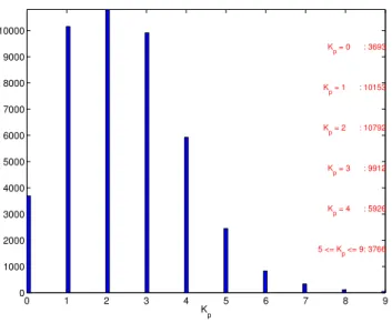
Because the number of strongly disturbed overflights with Kp≥6 was relatively small, as can be seen in Fig. 5,

includ-ing them in the average resulted in “bubbly” plots. Therefore, the conditionKp<6 was imposed here and also in the rest of

the study, unless otherwise stated.

(6)

0 1 2 3 4 5 6 7 8 9 0

1000 2000 3000 4000 5000 6000 7000 8000 9000 10000

K p = 0 : 3693

K

p = 1 : 10153

K

p = 2 : 10792

K p = 3 : 9912

K_p = 4 : 5926

5 <= K p <= 9: 3766

K p

Fig. 5.Distribution of overflights as a function ofKpand the

num-ber of overflights in theKp-bins.

upward field-aligned currentIr=+1.7and downward field-aligned currentIr=−1.6) than in the Southern Hemisphere (Ir=+1.3, Ir=−1.2), but this was most likely caused by the data selection criteria: The total number of 1-D over-flights in the Northern Hemisphere was 19 972, and 24 270 in the Southern Hemisphere. The excess overflights in the south took place during quiet geomagnetic conditions with Kp=0–2, during which, due to the differences between the

real geomagnetic field and the dipole field, the auroral oval was occasionally located poleward of the studied region be-tween₋76.5◦ _and₋₅₅◦ _{MAG latitude. Such overflights,}

with practically zero magnetic field, would pass the 1-D cri-terion, increasing the number of 1-D overflights in the South-ern Hemisphere, and decreasing the average current density there.

Since there were only minor differences between the hemi-spheres, the measurements from both hemispheres could be combined in order to produce more reliable statistics. This has been done in the following sections as well as in Fig. 4. This time, also Jcf,φ and Jdf,θ are shown, in addition to

Jcf,θ andJdf,φ. As expected, the currents are very similar

to those in Fig. 3.Jcf,φis clearly weaker in intensity than the

other curl-free component, Jcf,θ. It displays mainly dawn

to dusk directed currents on the dayside and on the nightside, which agree with the picture that part of the dawnside R1 rents cross the polar cap to close with the duskside R1 cur-rents. Similarly,Jdf,θ is weaker than the other

divergence-free componentJdf,φ, and consistent with the picture

involv-ing the antisunward electrojets in the dawn and dusk sectors of the oval and the sunward return flow in the polar cap.

4 Effect of theKpindex

A widely used proxy for geomagnetic activity is theKp

in-dex (Bartels et al., 1939). While by definition, increasing the index signifies the intensification and equatorward motion of the auroral oval, it is not so clear quantitatively how the cur-rent system changes as a function ofKp. In this section, this

effect is studied.

Figure 5 displays the distribution of the overflights be-tween differentKp values. The data have been divided into

six bins with Kp=0, Kp=1, Kp=2, Kp=3, Kp=4, and

Kp≥5. Here, the values withKp≥6 have also been included

in the appropriate bin. The number of overflights in each bin has been written in the plot in red.

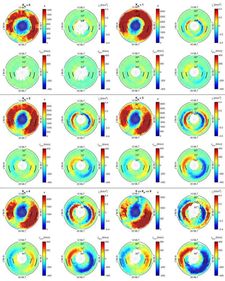
The current density binned with respect to theKpindex is

displayed in Fig. 6.

With increasingKp, the amplitude of the current density

increased and the auroral oval moved equatorward, as ex-pected. Also, the width of the oval clearly increased.

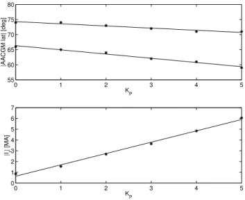
Figure 7 shows this behaviour more quantitatively: plotted are the equatorward and poleward boundaries of the oval as well as the total field-aligned current in one hemisphere in the different bins. The lines have been fitted to the data points with the least squares method. The AACGM latitude of the poleward boundary in degrees as a function ofKp is given

by

|lat_[deg_{]| = −}0.71_·Kp+74.3, (4)

the location of the equatorward boundary by

|lat_[deg_{]| = −}1.4_·Kp+66.3 (5)

and the amplitude of the total field-aligned current in MA by |Ir[MA]| =1.1·Kp+0.6. (6)

Equations (4) and (5) can be combined to give the width of the auroral oval as

1lat_[deg_{] =}0.69_·Kp+8.0. (7)

While Kp increased from 0 to ≥5, the oval widened and

moved equatorward from between _∼66◦_–74◦ _{AACGM lat}

to_∼59◦_–71◦ _{lat. The field-aligned currents increased by a}

factor of 7.

5 Seasonal effects

(7)

0 200 400 600 800 1000 1200 1400

K_P = 0

80o 70o 60o 00 MLT 06 MLT 12 MLT 18 MLT # −0.4 −0.2 0 0.2 0.4 80o 70o 60o 00 MLT 06 MLT 12 MLT 18 MLT j r [A/km

2_] −400 −200 0 200 400 80o 70o 60o 00 MLT 06 MLT 12 MLT 18 MLT

J_cf,θ [A/km]

−400 −200 0 200 400 80o 70o 60o 00 MLT 06 MLT 12 MLT 18 MLT

J_df,φ [A/km]

0 500 1000 1500 2000 2500 3000

K_P = 1

0 500 1000 1500 2000 2500 3000 3500

K_P = 2

0 500 1000 1500 2000 2500 3000 3500

K_P = 3

0 500 1000 1500 2000

K_P = 4

0 500 1000 1500

5 <= K

P <= 9

80o 70o 60o 00 MLT 06 MLT 12 MLT 18 MLT # −0.4 −0.2 0 0.2 0.4 80o 70o 60o 00 MLT 06 MLT 12 MLT 18 MLT

j_r [A/km2]

−400 −200 0 200 400 80o 70o 60o 00 MLT 06 MLT 12 MLT 18 MLT J cf,θ [A/km]

(8)

0 1 2 3 4 5 55

60 65 70 75 80

|AACGM lat| [deg]

K P

0 1 2 3 4 5

0 1 2 3 4 5 6 7

|Ir

| [MA]

K P

Fig. 7. The equatorward and poleward boundaries of the oval and the total field-aligned current as a function ofKp.

displayed a consistent evolution of the auroral and polar cap current systems as the IMF rotated around the circle. For negativeBz, the model included mainly the R1 and R2

sys-tems, but for positiveBz, an additional current system

ap-peared poleward of the R1 system. This R0 or NBZ sys-tem consisted of two regions of upward and downward field-aligned current with a polarity opposite to the surrounding R1 currents. For positive By, the upward R1 current on

the duskside wrapped through noon to become the dawnside R0 current, while the downward R1 current on the dawnside continued into the R2 current on the dawnside. The upward R0/R1 current encircled a small region of downward current, which appeared to be a remnant of the other pair in the NBZ system. Doubling the IMF magnitude intensified the cur-rents. During summer soltice, field-aligned current intensi-ties were much stronger than during winter solstice, and the NBZ system in particular was very prominent.

Papitashvili et al. (2002) derived a model for field-aligned currents from magnetic field measurements by the Øersted and Magsat satellites for summer, winter and equinox con-ditions. The magnetic field data were fitted with spherical harmonic functions and the field-aligned currents were com-puted using a simple 2-D curl technique. The model was parametrized by the IMF strength and direction. Using the model, Papitashvili et al. showed that the ratio of total field-aligned summer/winter currents is_∼1.35.

Christiansen et al. (2002) used the vector magnetic field measured by the Ørsted satellite from 25 August 1999 to 11 October 1999 and from 26 November 1999 to 24 Jan-uary 2000 to study the seasonal variations of the high-latitude field-aligned currents. They inferred the ratio of summer/winter field-aligned currents to be about 1.5–1.8.

Fujii et al. (1981) utilized the vector magnetic field data measured by the TRIAD satellite during years 1973–1974 and 1976–1977 to determine the seasonal dependence of the large-scale field-aligned currents in the Northern Hemi-sphere. They found that on the dayside, the ratio of sum-mer/winter field-aligned currents is about 2, while on the nightside, significant differences were not perceived.

Wang et al. (2005) used 2 years of magnetic field mea-surements from the CHAMP satellite to investigate the field-aligned currents in the southern polar ionosphere. They discovered that the intensity of the field-aligned currents changes with the merging electric field at all magnetic local time sectors, but with the solar radiation-induced conductiv-ity only on the dayside.

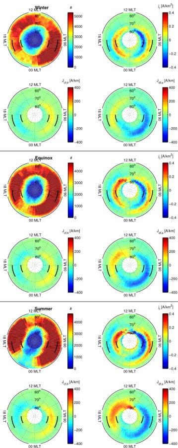
In order to compare whether our method produces similar results, Fig. 8 shows the winter (_±2 months around winter solstice), summer (_±2 months around summer solstice) and equinox (the rest of the year) current densities.

In agreement with Wang et al. (2005) and Fujii et al. (1981), the differences between the seasons in the figure were most clear on the dayside (06:00–18:00 MLT). In the winter, the currents were weaker on the dayside than on the nightside. The dayside currents intensified from win-ter (_|Ir|=2.5 MA) to equinox (|Ir|=2.9 MA) to summer

(_|Ir|=3.4 MA), so that the dayside currents became stronger

than the nightside currents. In agreement with Ridley (2007), Papitashvili et al. (2002) and Christiansen et al. (2002), the summer currents were found to be 1.4-times stronger than winter currents.

Considering the dayside (06:00–18:00 MLT) and nightside currents separately, the summer current turned out to be 1.7-times the winter current on the dayside, but only 1.2-1.7-times the winter current on the nightside. This is in accordance with the results of Fujii et al. (1981), and confirms that the effect was indeed mostly confined on the dayside.

On the dawnside (00:00–12:00 MLT),Jcf,θ that connects

the R1 and R2 field-aligned currents intensified fairly uni-formly from winter to equinox to summer, but on the dusk-side (12:00–24:00 MLT), the region of strongest Jcf,θ and

hence, the strongest field-aligned currents, shifted towards the dayside from 18:00–22:00 MLT to 14:00–22:00 MLT to 14:00–20:00 MLT. Table 1 lists separately the dawnside and duskside R1 (negativeIr on the dawnside and positiveIr on

the duskside) and R2 (positiveIr on the dawnside and

nega-tiveIron the duskside) currents.

(9)

0 1000 2000 3000 4000 5000

Winter

80o 70o 60o

00 MLT

06 MLT

12 MLT

18 MLT

#

−0.4 −0.2 0 0.2 0.4

80o 70o 60o

00 MLT

06 MLT

12 MLT

18 MLT

j r [A/km

2_]

−400 −200 0 200 400

80o 70o 60o

00 MLT

06 MLT

12 MLT

18 MLT

J cf,θ [A/km]

−400 −200 0 200 400

80o 70o 60o

00 MLT

06 MLT

12 MLT

18 MLT

J df,φ [A/km]

0 1000 2000 3000 4000

Equinox

80o 70o 60o

00 MLT

06 MLT

12 MLT

18 MLT

#

−0.4 −0.2 0 0.2 0.4

80o 70o 60o

00 MLT

06 MLT

12 MLT

18 MLT

j r [A/km

2_]

−400 −200 0 200 400

80o 70o 60o

00 MLT

06 MLT

12 MLT

18 MLT

J cf,θ [A/km]

−400 −200 0 200 400

80o 70o 60o

00 MLT

06 MLT

12 MLT

18 MLT

J df,φ [A/km]

0 1000 2000 3000 4000

Summer

80o 70o 60o

00 MLT

06 MLT

12 MLT

18 MLT

#

−0.4 −0.2 0 0.2 0.4

80o 70o 60o

00 MLT

06 MLT

12 MLT

18 MLT

j r [A/km

2_]

−400 −200 0 200 400

80o 70o 60o

00 MLT

06 MLT

12 MLT

18 MLT

J cf,θ [A/km]

−400 −200 0 200 400

80o 70o 60o

00 MLT

06 MLT

12 MLT

18 MLT

J df,φ [A/km]

Fig. 8.Ionospheric current density binned with respect to season.

Table 1. Dawnside (00:00–12:00 MLT) and duskside (12:00– 24:00 MLT) R1 (negativeIr on the dawnside and positive Ir on

the duskside) and R2 (positiveIr on the dawnside and negativeIr

on the duskside) currents in MA.

Dawn R1 Dawn R2 Dusk R1 Dusk R2 Winter −0.7 0.6 0.6 −0.5 Equinox −0.7 0.8 0.8 −0.6 Summer −0.9 1 0.8 −0.7

polar cap by the R0 currents. This would be in agreement with the result of Weimer (2001) that the R0 current system is very prominent in the summer.

6 Solar wind dynamic pressure effects vs. IMFBz

effects

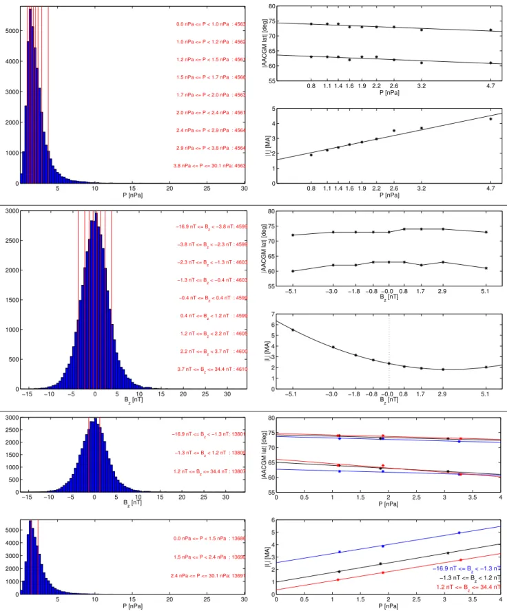
The two top left hand side panels of Fig. 9 display the dis-tribution of the overflights as a function of the solar wind dynamic pressure (P) and thezcomponent of the IMF (Bz).

The red lines in the plots display the bin boundaries and the number of overflights in each bin is written in red. The bins were chosen so that an approximately equal number of over-flights would fall into each. The right hand side panels dis-play the equatorward and poleward boundaries of the auroral oval and the total field-aligned current. TheP andBzvalues

on thex-axis are the medians for the bins.

With increasingP, also the intensity of the field-aligned current increased and both the poleward and the equatorward boundaries of the oval moved equatorward. Lines fitted to the points gave the AACGM lat of the poleward boundary of the oval in degrees as a function ofP in nPa as

|lat_[deg_{]| = −}0.57_·P_[nPa_{] +}74.4, (8) the equatorward boundary as

|lat_[deg_{]| = −}0.59_·P_[nPa_{] +}63.6 (9) and the amplitude of the total field-aligned current in MA as |Ir[MA]| =0.62·P[nPa] +1.6. (10)

There was only little variation in the intensity of the field-aligned current for positive and zero Bz, but for negative

Bz, the intensity of the field-aligned current clearly increased

with increasing amplitude ofBz. A polynomial of degree 2

was fitted to the data in the least-squares sense, giving the amplitude of the total field-aligned current in MA as a func-tion ofBzin nT as

|Ir[MA]| =0.054·Bz[nT]2−0.34·Bz[nT] +2.4. (11)

During negative Bz, the auroral oval was shifted slightly

southward from its zeroBzlocation, and during positiveBz,

(10)

5 10 15 20 25 30 0

1000 2000 3000 4000 5000

0.0 nPa <= P < 1.0 nPa : 4563

1.0 nPa <= P < 1.2 nPa : 4562

1.2 nPa <= P < 1.5 nPa : 4561

1.5 nPa <= P < 1.7 nPa : 4566

1.7 nPa <= P < 2.0 nPa : 4563

2.0 nPa <= P < 2.4 nPa : 4561

2.4 nPa <= P < 2.9 nPa : 4564

2.9 nPa <= P < 3.8 nPa : 4564

3.8 nPa <= P <= 30.1 nPa: 4563

P [nPa]

0.8 1.1 1.4 1.6 1.9 2.2 2.6 3.2 4.7

55 60 65 70 75 80

|AACGM lat| [deg]

P [nPa]

0.8 1.1 1.4 1.6 1.9 2.2 2.6 3.2 4.7

0 1 2 3 4 5

|Ir

| [MA]

P [nPa]

−15 −10 −5 0 5 10 15 20 25 30

0 500 1000 1500 2000 2500 3000

−16.9 nT <= B

z < −3.8 nT: 4599

−3.8 nT <= B

z < −2.3 nT : 4599

−2.3 nT <= B_z < −1.3 nT : 4603

−1.3 nT <= B_z < −0.4 nT : 4603

−0.4 nT <= B_z < 0.4 nT : 4599

0.4 nT <= B_z < 1.2 nT : 4599

1.2 nT <= B_z < 2.2 nT : 4605

2.2 nT <= B

z < 3.7 nT : 4600

3.7 nT <= B

z <= 34.4 nT : 4610

B z [nT]

−5.1 −3.0 −1.8 −0.8 −0.0 0.8 1.7 2.9 5.1

55 60 65 70 75 80

|AACGM lat| [deg]

B z [nT]

−5.1 −3.0 −1.8 −0.8 −0.0 0.8 1.7 2.9 5.1

0 1 2 3 4 5 6 7

|Ir

| [MA]

B z [nT]

−15 −10 −5 0 5 10 15 20 25 30

0 500 1000 1500 2000 2500 3000

−16.9 nT <= B

z < −1.3 nT: 13801

−1.3 nT <= B

z < 1.2 nT : 13809

1.2 nT <= B

z <= 34.4 nT : 13807

B z [nT]

5 10 15 20 25 30

0 1000 2000 3000 4000 5000

0.0 nPa <= P < 1.5 nPa : 13686

1.5 nPa <= P < 2.4 nPa : 13690

2.4 nPa <= P <= 30.1 nPa: 13691

P [nPa]

0 0.5 1 1.5 2 2.5 3 3.5 4

55 60 65 70 75 80

|AACGM lat| [deg]

P [nPa]

0 0.5 1 1.5 2 2.5 3 3.5 4

0 1 2 3 4 5 6

−16.9 nT <= B

z < −1.3 nT

−1.3 nT <= B z < 1.2 nT

1.2 nT <= B z <= 34.4 nT |Ir

| [MA]

P [nPa]

Fig. 9.Left: Distribution of the overflights as a function of the solar wind dynamic pressureP and thezcomponent of the IMF (Bz). The

(11)

The bottom panels of Fig. 9 show the data binned with re-spect to bothBzandP. There are three bins forBz, and the

values in those bins have further been divided into three bins with respect toP. The left hand side panel shows the distri-bution of overflights into the threeBzandP bins, separately.

The right hand side panel displays the equatorward and pole-ward boundaries of the auroral oval and the total field-aligned current as a function ofP. The threeBzbins are denoted by

the colors (negativeBz, zeroBz,positiveBz).

In agreement with the global MHD simulation results of Palmroth et al. (2004), our results indicate that regardless of the IMF direction, there is a positive correlation between the solar wind dynamic pressure and the intensity of the ionospheric currents. Although the relative response is not weaker for positive than for negative IMF (the fitted lines have slopes0.73, 0.77, and 0.73), the absolute intensity of the currents is clearly stronger for negative than for zero or positive IMF (the offsets of the lines are2.6 MA, 1.0 MA, and0.4 MA). Therefore, the most intense currents were ob-tained with negativeBzand high dynamic pressure. For the

negativeBzand maximumP-bin, the currents were 4.2 times

stronger than for the positiveBzand minimumP-bin.

7 Effects of the merging electric field

The left hand side panel of Fig. 10 shows the distribution of the overflights as a function of the merging electric fieldEm.

The red lines in the plot again display the bin boundaries and the number of overflights in each bin is written in red. As in the previous section, also here the bins were chosen so that an approximately equal number of overflights would fall into each. The right hand side panel displays the equatorward and poleward boundaries of the auroral oval and the total field-aligned current. TheEmvalues on thex-axis are the medians

for the bins.

Lines fitted to the points give the AACGM lat of the pole-ward boundary of the oval in degrees as a function ofEmin

mV/m as

|lat_[deg_{]| = −}0.80_·Em[mV/m] +74.1, (12)

the equatorward boundary as

|lat_[deg_{]| = −}0.82_·Em[mV/m] +63.1 (13)

and the amplitude of the total field-aligned current in MA as |Ir[MA]| =1.41·Em[mV/m] +1.4. (14)

The behaviour of the locations of the poleward and equator-ward boundaries of the oval and_|Ir|as a function ofP and

Em resemble each other closely. With increasing values of

both, the auroral oval moves equatorward and_|Ir|

intensi-fies linearly. For positiveBz, on the other hand,|Ir|is

rela-tively independent on the magnitude ofBz, remaining around

2 MA, whereas for negativeBz, the intensity of|Ir|increases

with increasingBzmagnitude.

8 Discussion

The solar wind energy enters the magnetosphere by magnetic reconnection and viscous interaction (Dungey, 1961; Axford and Hines, 1961), but the location where reconnection takes place on the dayside magnetopause still remains unresolved. There are two main hypothesis that predict the effect of the IMF direction on the location: According to the component reconnection hypothesis (Sonnerup, 1974), reconnection is most likely to occur on a line passing through the subsolar point, where the solar wind dynamic pressure is most in-tense. The angle between the magnetosheath and the geo-magnetic field is less relevant: the antiparallel components of the fields are reconnected regardless of the presence of any parallel components. In contrast, the antiparallel reconnec-tion hypothesis (Luhmann et al., 1984) states that the pres-ence of parallel components is enough to prevent reconnec-tion, which implies that reconnection can only take place in those regions on the magnetopause where the magnetosheath and geomagnetic fields are oppositely directed. Therefore, any IMF orientation can produce reconnection, provided that there is a region where the two fields are antiparallel, and that there is sufficient plasma convection towards that region to bring the two field configurations in contact.

During negative IMFBzand zeroBy, both hypothesis

pre-dict a uniform reconnection line at the equatorial plane, but with increasingBy, the antiparallel reconnection line breaks

and the ends move away from equator toward the cusps, while the component reconnection line remains uniform and is merely tilted. During positiveBz, parallel reconnection is

predicted to take place tailward of the cusps, while compo-nent reconnection occurs mostly due toBy.

Since the reconnection rate is related to the Alfv´en veloc-ity of the inflowing plasma (VA=B/√µ0ρ, ρ is the mass

density), reconnection at the magnetopause could be en-hanced by increasing IMFB. According to both the com-ponent and antiparallel reconnection hypothesis, intensify-ing negative IMFBz, which implies either increasingB or

rotation of the IMF vector towards a more southward ori-entation, generally increases the reconnection rate. During positiveBz, component reconnection is caused byBy, which

would imply that the intensity ofBzhas no effect on the

re-connection rate. According to the antiparallel hypothesis, on the other hand, during positive IMFBz, reconnection occurs

tailward of the cusps. While the reconnection rate should then depend on the Bz amplitude, the ionospheric

signa-tures would be mostly confined to high (>80◦_{) latitudes (e.g.,}

Stauning, 2002), which have not been included in our study. Therefore, our results, according to which there was very lit-tle variation in the auroral ionospheric field-aligned current intensity during positive and zeroBz, while during negative

Bz, the intensity increased with the increasing amplitude of

Bz, are in agreement with both hypothesis.

(12)

1 2 3 4 5 6 7 8 9 10 0

500 1000 1500 2000 2500 3000 3500 4000 4500

0.0 mV/m <= E_m < 0.1 mV/m : 4562

0.1 mV/m <= E_m < 0.3 mV/m : 4562

0.3 mV/m <= E_m < 0.5 mV/m : 4562

0.5 mV/m <= E_m < 0.7 mV/m : 4562

0.7 mV/m <= E_m < 1.0 mV/m : 4562

1.0 mV/m <= E_m < 1.3 mV/m : 4562

1.3 mV/m <= E_m < 1.7 mV/m : 4562

1.7 mV/m <= E_m < 2.4 mV/m : 4562

2.4 mV/m <= E

m <= 10.4 mV/m: 4564

E m [mV/m]

0.00.2 0.4 0.6 0.9 1.1 1.5 2.0 3.0

55 60 65 70 75 80

|AACGM lat| [deg]

E m [mV/m]

0.00.2 0.4 0.6 0.9 1.1 1.5 2.0 3.0

0 2 4 6 8

|Ir

| [MA]

E m [mV/m]

Fig. 10.Left: Distribution of the overflights as a function of the merging electric field (Em). The red lines display the bin boundaries and

the number of overflights in each bin is written in red. Right: The equatorward and poleward boundaries of the auroral oval and the total field-aligned current as a function ofEm.

magnetopause exceeds that in the tail, the boundary between the open and closed field lines moves equatorward. The electric field associated with the solar wind plasma flow across these reconnected open field lines of the polar cap (E₌₋V_×B,V is the solar wind velocity andB the IMF) is mapped down to the ionosphere along the geomagnetic field lines. According to Eqs. (1) and (2), the Pedersen, Hall and field-aligned current densities are then all affected by

E, which could be enhanced by increasing B, P₌ρV2 or Em=V

q B2

y+Bz2sin2(θ/2).

SinceEm takes into account both the IMF direction and

magnitude and the solar wind speed, it could be expected to describe the solar wind-magnetosphere coupling better than eitherBz orP. Indeed, in Figs 9 and 10, the most intense

currents can be found in the highEm-bin.

9 Summary

Magnetic field measurements from the CHAMP satellite dur-ing years 2001–2005 have been used to derive statistical maps of ionospheric currents as a function of the AACGM latitude and MLT. The effects of theKpindex, season, thez

component of the IMF (Bz), the solar wind dynamic pressure

(P), and the merging electric field (Em) on the large-scale

ionospheric currents have been studied.

The ionospheric currents in the Northern and in the South-ern Hemispheres were found to differ only slightly when averaged over long time periods, which meant that the data from both hemispheres could be combined in order to improve the statistics. Between 04:00–06:00 and 18:00–

20:00 MLT, the oval was found to be located between 62◦_–

73◦_{latitude, on average.}

Increasing theKp index from 0 to≥5 intensified the

to-tal field-aligned current by a factor of 7. The auroral oval widened and moved equatorward from between 66◦_–74◦

AACGM lat to 59◦_–71◦_{lat. Simple expressions describing}

the locations of the poleward (Eq. 4) and equatorward bound-ary of the oval (Eq. 5) as well as the total field-aligned current (Eq. 6) were determined.

Seasonal effects on the currents were found to be most prominent on the dayside. In agreement with previous stud-ies, total field-aligned current in the summer was found to be 1.4 times stronger than in the winter. On the dayside (06:00– 18:00 MLT), the ratio was 1.7 and on the nightside, 1.2.

With increasingP or Em, the poleward and equatorward

boundaries of the auroral oval moved equatorward and the to-tal field-aligned current intensified linearly (Eqs. 10 and 14). There was only little variation in the intensity of the field-aligned current for positive and zeroBz, but for negativeBz,

the intensity clearly increased with increasing amplitude of Bz. Equation (11) was derived to describe the dependence of

the total field-aligned current onBz. Thus, the most intense

currents were obtained with negativeBz and high dynamic

pressure. For the negativeBzand maximumP -bin, the

cur-rents were 4.2 times stronger than for the positive Bz and

minimumP-bin.

(13)

Acknowledgements. The operational support of the CHAMP mis-sion by the German Aerospace Center (DLR) and the financial support for the data processing by the Federal Ministry of Ed-ucation (BMBF), as part of the Geotechnology Programme, are gratefully acknowledged. The OMNI data were obtained from the GSFC/SPDF OMNIWeb interface at http://omniweb.gsfc.nasa.gov. The work of L. Juusola was supported by the Finnish Graduate School in Electromagnetics and the Academy of Finland (project no. 121289). The authors thank S. Hassinen for technical assis-tance.

Topical Editor M. Pinnock thanks V. Papitashvili for his help in evaluating this paper.

References

Axford, W. I. and Hines, C. O.: A unifying theory of high-latitude geophysical phenomena and geomagnetic storms, Can. J. Phys., 39, 1433–1464, 1961.

Bartels, J., Heck, N. H., and Johnston, H. F.: The three-hour-range index measuring geomagnetic activity, Terr. Magn. Atmos. Electr., 44, 411–454, 1939.

Boudouridis, A., Zesta, E., and Lyons, L. R.: Effect of solar wind pressure pulses on the size and strength of the auroral oval, J. Geophys. Res., 108, 8012, doi:10.1029/2002JA009373, 2003. Brekke, A.: Physics of the Upper Polar Atmosphere, Wiley-Praxis

Series in Atmospheric Physics, John Wiley and Sons, New York, 1997.

Christiansen, F., Papitashvili, V. O., and Neubert, T.: Seasonal variations of high-latitude field-aligned currents inferred from Ørsted and Magsat observations, J. Geophys. Res., 107, 1029, doi:10.1029/2001JA900104, 2002.

Dungey, J. W.: Interplanetary Magnetic Field and the Auroral Zones, Phys. Rev. Lett., 6, 47–48, 1961.

Fujii, R., Iijima, T., Potemra, T. A., and Sugiura, M.: Seasonal Dependence of Large-Scale Birkeland Currents, Geophys. Res. Lett., 8, 1103–1106, 1981.

Fukushima, N.: Generalized theorem for no ground magnetic ef-fect of vertical currents connected with Pedersen currents in the uniform-conductivity ionosphere, Rep. Ionos. Space Res. Japan, 30, 35–40, 1976.

Gustafsson, G., Papitashvili, N. E., and Papitashvili, V.: A revised corrected geomagnetic coordinate system for Epochs 1985 and 1990, J. Atmos. Terr. Phys., 54, 1609–1631, 1992.

Holme, R., Olsen, N., Rother, M., and L¨uhr, H.: CO2 – A CHAMP magnetic field model, 220–225, First CHAMP Mission Results for Gravity, Magnetic and Atmospheric Studies edited by C. Reigber and H. L¨uhr and P. Schwintzer, Springer, Berlin, 2003. Iijima, T. and Potemra, T. A.: The Amplitude Distribution of

Field-Aligned Currents at Northern High Latitudes Observed by Triad, J. Geophys. Res., 81, 2165–2174, 1976.

Juusola, L., Amm, O., and Viljanen, A.: One-dimensional spherical elementary current systems and their use for determining iono-spheric currents from satellite measurements, Earth, Planets and Space, 58, 667–678, 2006.

Juusola, L., Amm, O., Kauristie, K., and Viljanen, A.: A model for estimating the relation between the Hall to Pedersen conductance ratio and ground magnetic data derived from CHAMP satellite statistics, Ann. Geophys., 25, 721–736, 2007,

http://www.ann-geophys.net/25/721/2007/.

Kamide, Y. and Baumjohann, W.: Magnetosphere-Ionosphere Cou-pling, Springer-Verlag, Berlin Heidelberg, 1993.

Kan, J. R. and Lee, L. C.: Energy Coupling Function and Solar Wind-Magnetosphere Dynamo, Geophys. Res. Lett., 6, 577–580, 1979.

Liou, K., Newell, P. T., and Meng, C.-I.: Seasonal effects on auro-ral particle acceleration and precipitation, J. Geophys. Res., 106, 5531–5542, 2001.

Lu, G., Richmond, A. D., Emery, B. A., Reiff, P. H., de la Beau-jardi`ere, O., Rich, F. J., Denig, W. F., Kroehl, H. W., Lyons, L. R., Ruohoniemi, J. M., Friis-Christensen, E., Opgenoorth, H., Persson, M. A. L., Lepping, R. P., Rodger, A. S., Hughes, T., McEwin, A., Dennis, S., Morris, R., Burns, G., and Tomlin-son, L.: Interhemispheric Asymmetry of the High-Latitude Iono-spheric Convection Pattern, J. Geophys. Res., 99, 6491–6510, 1994.

Luhmann, J. G., Walker, R. J., Russell, C. T., Crooker, N. U., Spre-iter, J. R., and Stahara, S. S.: Patterns of Potential Magnetic Field Merging Sites on the Dayside Magnetopause, J. Geophys. Res., 89, 1739–1742, 1984.

Ohtani, S., Ueno, G., Higuchi, T., and Kawano, H.: Annual and semiannual variations of the location and intensity of large-scale field-aligned currents, J. Geophys. Res., 110, A01216, doi:10. 1029/2004JA010634, 2005.

Palmroth, M., Pulkkinen, T. I., Janhunen, P., McComas, D. J., Smith, C. W., and Koskinen, H. E. J.: Role of solar wind dy-namic pressure in driving ionospheric Joule heating, J. Geophys. Res., 109, A11302, doi:10.1029/2004JA010529, 2004.

Papitashvili, V. O., Christiansen, F., and Neubert, T.: A new model of field-aligned currents derived from high-precision satellite magnetic field data, Geophys. Res. Lett., 29, 1683, doi:10.1029/ 2001GL014207, 2002.

Ridley, A. J.: Effects of seasonal changes in the ionospheric conduc-tances on magnetospheric field-aligned currents, Geophys. Res. Lett., 34, L05101, doi:10.1029/2006GL028444, 2007.

Ritter, P., L¨uhr, H., Maus, S., and Viljanen, A.: High-latitude iono-spheric currents during very quiet times: their characteristics and predictability, Ann. Geophys., 22, 2001–2014, 2004,

http://www.ann-geophys.net/22/2001/2004/.

Schunk, R. W. and Nagy, A. F.: Ionospheres – Physics, Plasma Physics, and Chemistry, Cambridge Univ. Press, 2000.

Sonnerup, B. U. O.: Magnetopause reconnection rate, J. Geophys. Res., 79, 1546–1549, 1974.

Stauning, P.: Field-aligned ionospheric current systems observed from Magsat and Oersted satellites during northward IMF, Geo-phys. Res. Lett., 29, 8005, doi:10.1029/2001GL013961, 2002. Vanham¨aki, H., Amm, O., and Viljanen, A.: 1-Dimensional

up-ward continuation of the ground magnetic field disturbance us-ing spherical elementary current systems, Earth Planets Space, 55, 613–625, 2003.

Wang, H., L¨uhr, H., and Ma, S. Y.: Solar zenith angle and merging electric field control of field-aligned currents: A statistical study of the Southern Hemisphere, J. Geophys. Res., 110, A03306, doi: 10.1029/2004JA010530, 2005.