www.earth-surf-dynam.net/3/333/2015/ doi:10.5194/esurf-3-333-2015
© Author(s) 2015. CC Attribution 3.0 License.
Sensitivity analysis and implications for surface
processes from a hydrological modelling approach in the
Gunt catchment, high Pamir Mountains
E. Pohl1, M. Knoche2, R. Gloaguen1,3, C. Andermann4, and P. Krause5 1Remote Sensing Group, Geology Institute, Technische Universität Bergakademie Freiberg,
B.-von-Cotta-Str. 2, 09599 Freiberg, Germany
2Helmholtz Centre for Environmental Research (UFZ), Halle, Germany
3Remote Sensing Group, Helmholtz Institute Freiberg of Resource Technology, Freiberg, Germany 4Helmholtz Centre Potsdam, German Research Centre for Geosciences (GFZ), Potsdam, Germany
5Gewässerkundlicher Landesdienst, Hochwassernachrichtenzentrale,
Thüringer Landesamt für Umwelt und Geologie (TLUG), Jena, Germany
Correspondence to:E. Pohl ([email protected])
Received: 30 October 2014 – Published in Earth Surf. Dynam. Discuss.: 15 December 2014 Revised: 26 June 2015 – Accepted: 3 July 2015 – Published: 23 July 2015
as water availability in the downstream areas. The proposed conceptual model has a tremendous importance for the understanding of the denudation processes in the region. In the Pamirs, large releases of running water that control erosion intensity are primarily controlled by temperature and the availability of snow and glaciers, thus making the region particularly sensitive to climatic variations.
1 Introduction
The Amu Darya, the main river draining the Pamir Moun-tains (hereafter the Pamirs) to the west, provides water re-sources for hydropower and irrigation along its way to the Aral Sea. Its various tributaries originate in the high moun-tains and experience wide-ranging climatic, topographic, and tectonic settings (Fuchs et al., 2013, 2014b). The Pamirs are located in the transition zone between the Westerlies in the west (in the winter half-year) and the Indian summer mon-soon (ISM) in the south (in the summer half-year) (Fuchs et al., 2013; Aizen et al., 2009; Syed et al., 2006; Palazzi et al., 2013; Mischke et al., 2010). This unique setting make the Pamirs an outstanding natural laboratory to study as-pects of climate variability, hydrologic response, and gov-erned Earth surface processes under different climatic in-fluences. The hydrological regime is reported to be snow-and glacier-melt-dominated (Lutz et al., 2014; Kure et al., 2013; Tahir et al., 2011), albeit quantitatively largely uncon-strained. Increasing demand for water and assumed changes in hydrological regimes of glaciated catchments with respect to a change in climatic conditions (Immerzeel et al., 2009; Hagg et al., 2013), as well as the inherent increased risks, demand for a better understanding of the processes govern-ing surface flow in the region.
Because water acts as the main transport agent for sed-iments out of mountain belts (e.g. Milliman and Syvitski, 1992; Galy and France-Lanord, 2001) and plays a crucial role in the global carbon cycle (Maher and Chamberlain, 2014), sound estimates of the hydrological water balance and water components are also of fundamental importance for Earth surface processes. The primary control of tectoni-cally driven topographic steepness on erosion suggests that changes in water availability are balanced by complex inter-actions between channel steepness and width, as well as con-centrated sediment transport (Burbank et al., 2003; Scher-ler et al., 2014). But hydrology-related surface processes are manifold, including frost cracking intensities based on avail-able water content (e.g. Andersen et al., 2015; Egholm et al., 2015), sediment mobilisation from snowmelt (Gao et al., 2014; Iida et al., 2012), glacier melt as a transport agent for sediment (Chernova, 1981; Ali and De Boer, 2010), river in-cision (Snyder et al., 2003; Lague et al., 2005), landslide trig-gering due to soil moisture content (Iverson, 2000; Dietrich et al., 1992), and suspended sediment transport in rivers (An-dermann et al., 2012a, c; Dadson et al., 2003; Milliman and Syvitski, 1992). Therefore, obtaining spatiotemporal
knowl-edge about water mobilisation in quantity and quality can provide further insights into the effects of climate and cli-mate variability on mountain evolution (Champagnac et al., 2012; DiBiase and Whipple, 2011; Montgomery and Bran-don, 2002). It would also allow for improved hazard risk assessment, which often relies on long-term projections of temperature increase and their effect on melting processes (Gruber and Mergili, 2013).
There is a consensus in the characteristic change in the hy-drologic regime along the Himalayan front from rainfall to snow- and glacier-melt-dominated systems towards the west (Xiao et al., 2002; Bookhagen and Burbank, 2010; Lutz et al., 2014; Immerzeel et al., 2009). The few hydrologic studies in the Pamirs are hence basically glacier melt/snowmelt–runoff models that relied on in situ data (Hagg et al., 2007) and, more recently, on GCM (global climate model) data out-put (Kure et al., 2013; Hagg et al., 2013; Lutz et al., 2013) including future climate change scenarios. In contrast with the qualitatively agreeing hydrological studies, studies fo-cusing solely on glaciers in the Pamirs show ambiguous re-sults. Gardelle et al. (2013), for example, show a slight mass gain for glaciers in the Pamirs and also the Karakoram re-gion for the last decade. Conversely, Lutz et al. (2013) and Sorg et al. (2012) report negative glacier mass balances for the Abramov Glacier in the north-eastern part of the Pamirs, however for a slightly earlier time period.
The different climatological settings between the Pamirs and the Himalayan escarpments stand in contrast to surpris-ingly similar regional erosion rates (Herman et al., 2013) for the last 2 million years. While order-of-magnitude-higher precipitation amounts in the Himalayas do not allow for a clear picture of how climate defines landscape evolution (Godard et al., 2014), the much drier climate in the Pamirs provides fundamentally different boundary conditions and suggests water availability as a limiting factor (Fuchs et al., 2014b). Precipitation intensities alone, however, cannot solve the discrepancy of intensities between hillslope erosion and river incision in the Pamirs (Fuchs et al., 2014a, b). Obtaining detailed spatiotemporal information from hydrological mod-elling is bound to an accurate assessment of forcing parame-ters. These are required with a matching spatiotemporal dis-tribution, and hence remote sensing or GCM data provide an advantage over in situ data or the lack thereof, which is a major challenge in data-scarce regions such as the Pamirs.
a good example of how diverse results can be if different downscaling approaches are applied in heterogenous areas, leading to over- or underestimation by a few hundred per-cent. The same is also true for the interpolation of in situ data, depending on what temperature lapse rates and precipitation gradients are applied (Immerzeel et al., 2014). Furthermore, the large differences in GCM and remote sensing data sets (Palazzi et al., 2013; Ménégoz et al., 2013) call for a valida-tion with in situ data, which might not always be available. Newly developed regional climate models (RCMs), such as HAR10 (Maussion et al., 2014), help in preventing inaccu-rate interpolation. But available time spans and spatial cov-erage are limited. This is due to the high computational ex-pense that is needed to create such data sets. The abundance and increasing accuracy in GCMs, RCMs, and remote sens-ing data has led to their greater use in hydrological mod-elling (Khan et al., 2011; Awange et al., 2011; Liu et al., 2012; Bookhagen and Burbank, 2010) and glacier evolution studies (Gardelle et al., 2012, 2013; Lutz et al., 2014; Sorg et al., 2012). In cold, arid, mountainous regions, GCMs are often favoured over remote sensing data. This is due to dif-ficulties in snowfall (Prigent, 2010) and snow water equiva-lent (SWE) retrieval (Takala et al., 2011; Tong et al., 2010) from space. Furthermore, direct measurement of ground air temperature from space is not possible. Remote sensing land surface temperatures (LSTs) are, however, being used, for example, to derive temperature lapse rates for interpolation of in situ data (Liu et al., 2012) or the calculation of evapo-ration (Samaniego et al., 2011). Use of LSTs as a proxy for ground air temperature has also been established, however only in lowlands (Deus et al., 2013).
This paper concentrates on resolving the hydrologic cycle in the high Pamirs, using a conceptual, semi-distributed hy-drological model. This approach is very demanding due to data scarcity, and hence a special focus is directed toward the validation of independent daily raster data from remote sensing, climate models, and combined products. The limited possibilities and problems (Tustison et al., 2001) in validat-ing the specific raster data sets with in situ measurements are accounted for by an analysis of their influence on systematic effects in the resulting hydrological models. We ultimately aim for a conceptual description of the hydrological cycle in the Gunt River basin in order to understand and quantify the main drivers of erosion and incision in the Pamirs. Uncertain-ties in the data and model are discussed in detail. The quan-tification of the different water components is of fundamental relevance for understanding surface processes (mass wasting, glacier lake outburst floods, etc.), and eventually for under-standing the controlling factors of denudation rates. Here, we consider the Gunt River basin as representative for the central Pamirs. We describe potentials and limitations of hydrologi-cal modelling under data scarcity as a tool for understanding erosive processes. Finally, we use obtained results on mois-ture supply, as well as water mobilisation, to infer a concep-tual model for expected surface processes in the Pamirs.
2 Study area
0 20 40 60 80 100 120 140 160 180 200 −30 −20 −10 0 10 20 30 40 [mm] [ºC]
J F M A M J J A S O N D Khorog
2080 m a.s.l.
ø 432[mm yr−1]
ø 9.4 [ºC]
0 20 40 60 80 100 120 140 160 180 200 −30 −20 −10 0 10 20 30 40 [mm] [ºC]
J F M A M J J A S O N D Bulunkul
3751 m a.s.l.
ø 93[mm yr−1]
ø −7.9 [ºC]
0 20 40 60 80 100 120 140 160 180 200 −30 −20 −10 0 10 20 30 40 [mm] [ºC]
J F M A M J J A S O N D Dzaushangoz
3480 m a.s.l.
ø 124[mm yr−1]
ø −1.9 [ºC]
0 20 40 60 80 100 120 140 160 180 200 −30 −20 −10 0 10 20 30 40 [mm] [ºC]
J F M A M J J A S O N D Murghab
3589 m a.s.l.
ø 91[mm yr−1]
ø −1 [ºC]
0 20 40 60 80 100 120 140 160 180 200 −30 −20 −10 0 10 20 30 40 [mm] [ºC]
J F M A M J J A S O N D Navabad
2570 m a.s.l.
ø 392[mm yr−1]
ø 5.6 [ºC]
0 20 40 60 80 100 120 140 160 180 200 −30 −20 −10 0 10 20 30 40 [mm] [ºC]
J F M A M J J A S O N D Shaimak
3871 m a.s.l.
ø 182[mm yr−1]
ø −3 [ºC]
0 20 40 60 80 100 120 140 160 180 200 −30 −20 −10 0 10 20 30 40 [mm] [ºC]
J F M A M J J A S O N D Ishkashim
2530 m a.s.l.
ø 137[mm yr−1]
ø 7.4 [ºC]
Figure 1.Climate diagrams for the available meteorological stations with precipitation amounts (blue) and temperature (red). The west-ernmost stations, Khorog, Navabad, and Ishkashim, show a distinctive precipitation maximum in winter. The influence of Westerlies in the winter half-year decreases with altitude towards the east (Bulunkul, Murghab, Shaimak). There is an increase in precipitation during monsoon season with peak in summer for Murghab and Shaimak in the easternmost part.
Ý Ý Ý Ý Ý Ý Ý Ý Ý Ý Ý Ý Ý
0 200 400
0 1500 3000 4000 5000 6000 9000 Tajikistan China Pakistan India Ý Ý Ý Ý Ý Ý Ý Ý Ý Ý Ý Ý 0 100 km S E N W Ishkashim Khorog Navabad Dzaushangoz Bulunkul Murghab Shaimak Westerlies
Indian Summer Monsoon Afghanistan
Shakhdara Gunt
Wakhan Range
Shugnan Range
Rushan R ange
Shakhdar a Range
Lake Yashilkul
Meteorological station Discharge measurement Snow & ice (MODIS)
Lake
Figure 2.Study area in the Tajik Pamirs with catchment area of the Gunt and Shakhdara rivers and available meteorological stations and discharge measurement location. Monsoon and Westerlies are indicated by arrows according to Zech et al. (2005) and Fuchs et al. (2013). MODIS MCD12Q1 land cover class for permanent ice and snow cover (light blue) as a proxy for glacier extent.
of the Gorno-Badakhshan Autonomous Oblast (GBAO) in south-eastern Tajikistan (37◦N, 73◦E), in the Pamirs (Fig. 2). It extends over about 14 000 km2. The rivers Gunt and Shakhdara connect before they flow through Khorog, where an available gauging station is located. The catchment is characterised by elevations ranging between 2080 m a.s.l.
at the catchment outlet and up to 6700 m a.s.l.at Karl Marx Peak in the Shakhdara Range. The average elevation is about 4300 m a.s.l. The higher elevations bound the catchment,
2 4 6 8 10 12
0
20
60
100
month
Sno
w co
ver [%]
mean median 1st to 3rd quartile 0.1 to 0.9−percentile
Figure 3.Monthly average snow cover in the Gunt catchment. Data basis is MOD10CM (Hall et al., 2006) monthly snow cover for the period 2001 to 2012.
high elevations impossible. Even though the eastern stations are generally higher in altitude and receive less precipitation than those in the western part, there is no evident relationship between altitude and precipitation.
With an average altitude of 4300 m a.s.l., the region shows a long-lasting snow cover period (Fig. 3) with an average snow cover of >50 % from November until March (Im-merzeel et al., 2009; Pu et al., 2007; Dietz et al., 2014). A negative temperature gradient is apparent along the west– east gradient in precipitation and relief. Station Bulunkul shows exceptionally low values of both precipitation and temperature. This is likely induced by its location, which is surrounded by mountains in the close proximity. Due to the long-lasting snow cover and the bulk of precipitation pro-vided as winter precipitation, snowmelts are expected to play an essential role in the water balance. Even though the east-ernmost parts receive higher fractions of summer over win-ter precipitation, temperatures below freezing temperature at valley floor level during most of the year (Fig. 1) suggest a substantial amount of precipitation received as snow. While there is a pronounced west–east gradient in precipitation, no precipitation lapse rate is evident from the limited in situ data (Fig. 1).
Daily discharge measurements have been conducted in Khorog (Fig. 2) with few exceptions since 1960. We cannot independently assess the quality of the measurements, but old equipment that has not been maintained since the inde-pendence of Tajikistan, along with old rating curves, imply a possible source of error. Anthropogenic influences on the observed discharge are most probably minor but hard to as-sess. A hydropower plant and a lake regulation station are in operation near site Navabad and at Lake Yashilkul (see Fig. 2), respectively. While the amount of water used by the power plant would return to the river without change in quan-tity and without noticeable recession, the assessment of lake discharge is difficult. Discharge records from the 1960s for Khorog show similar winter discharge to the 2000s. This al-lowed us to assume that the water usage from the hydropower plant and the lake regulation do not affect the
hydrologi-cal cycle much. Furthermore, a few years of data for a sub-catchment of the Gunt River (gauging the Gunt river itself ≈50 km downstream of Lake Yashilkul) show winter dis-charge of≈8 m3s−1, which makes up one-third of the
dis-charge at Khorog in winter. This 8 m3s−1 includes a few other sub-catchments, of which one contributes an additional 1–2 m3s−1. This suggests that the overall contribution of lake
discharge to the observed runoff is very low and that the observed winter discharge results mainly from groundwater discharge. Neither melt nor liquid precipitation is expected during winter due to low temperatures. Other anthropogenic influences include irrigation, which occurs during summer and almost exclusively in the valleys. According to the land cover classification used (see Sect. 4.1.3 for derivation), only 0.1 % are croplands. Hergarten (2004) report irrigated land to account for only 0.38 % in the Pamir region. To roughly estimate the impact of irrigation, we estimated the water con-sumption based on obtained model results for potential evap-otranspiration, an irrigated area according to 0.38 % land cover, and an assumed irrigation period between May and September. The resulting impact corresponds to 0.4 % of the average annual discharge measured at Khorog.
The available discharge data for Khorog at the catchment outlet shows a general intra-annual pattern with very low and generally declining discharge from October to March. Low-est discharge occurs at the end of March (≈30 m3s−1). In
April, the discharge rapidly increases and shows strong vari-ability until September, when discharge strongly attenuates. Peak discharge occurs in July (≈290 m3s−1). Average
dis-charge for the winter period (ONDJFM) is about 44 m3s−1,
and for the summer period (AMJJAS) about 164 m3s−1. The
average annual discharge is 3.48 km3yr−1(i.e. 255 mm yr−1
or 105 m3s−1). Strong interannual variations in the summer
hydrograph contrast with a low and rather constant winter hydrograph. This further suggests a high importance of snow and glacier melts for the hydrological cycle and a signifi-cant fraction of groundwater discharge in winter. The inter-annual discharge variability is high, e.g. 132 m3s−1in 2005
vs. 95 m3s−1in 2007. During fieldwork in March 2013, we
observed that the inflow to Lake Yashilkul (3800 m a.s.l.) was entirely frozen. Likewise, interrupted streamflow is assumed for other high-elevation tributaries in winter and the entire catchment area east of Lake Yashilkul. The eastern part of the catchment is in a zone of potential permafrost (altitudes above 3800 m a.s.l.; Mergili et al., 2012). Hence, water re-lease from permafrost or from sporadically frozen soils is assumed to play a role in the hydrological cycle.
3 Methods
0.01°
0.05°
0.10°
0.25°
0.75°
HRUs
MODIS
HAR10
ECMWF TRMM APHRODITE GLDAS
Meteorological Data
P T RH
SD U
HRU processing Elevation
Slope Aspect Soil Land cover Hydrogeology
derived from
snow module
glacier module
soil module
groundwater module
. . .
Discharge components
Evapotrans-piration
Storage components
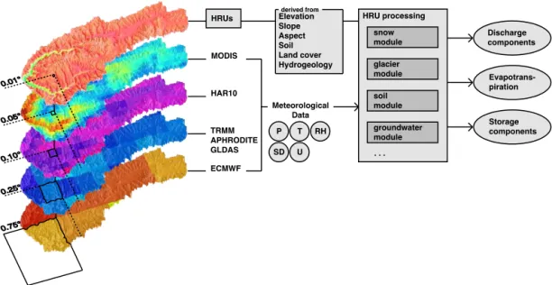
Figure 4.Schematic superimposition of different meteorological raster data with various spatial resolutions. Hydrological response unit (HRUs) have 1 km×1 km pixel size. Processing modules of the J2000g model take needed forcing data (P: precipitation;T: temperature; RH: relative humidity; SD: sunshine hours;U: near-ground wind speed) to be processed for each individual HRU. The final step is the output of discharge components, evapotranspiration, and storage changes.
3.1 Hydrological modelling
Depending on the area of interest, choices had to be made regarding the computational and distributional concept, as well as the model’s temporal resolution. Daniel (2011) gives a good comparison of different frequently used models but the number of different models is simply too large to be cov-ered entirely. The integration of raster data sets has been implemented in different models such as the MIKE SHE (Cooper et al., 2006; Liu et al., 2012) or CREST (Khan et al., 2011) models, and several more examples of raster data in-put are available (Merritt et al., 2006; Stahl et al., 2008; Wood et al., 2004). While each of these models has spe-cific qualities, none of them globally outperforms the oth-ers. The majority of existing models require very specific and scarcely available information on specific properties of, for example, soils and plants. We only have limited infor-mation available about these properties. Hence, we chose the conceptual distributed hydrological model J2000g within the JAMS framework. The model is adapted to multi-scale hy-drological studies and needs only a limited number of soil and plant properties, which also reduces the complexity of the calibration process. The benefit of higher simplicity con-trasts an apparent simplification of physical processes related to soil and water routing dynamics. An important feature of J2000g is the possibility of using raster data sets as meteoro-logical input (Krause et al., 2010) and adapting some model components to the study area. Similar approaches have been successfully implemented not only in flat, semi-arid terrain (Deus et al., 2013) but also in glaciated, mountainous regions (Nepal et al., 2014).
3.2 The JAMS framework and the hydrological model J2000g
The hydrological model J2000g (Kralisch et al., 2007; Krause and Hanisch, 2009) is modular-based and allows, to a certain degree, for the interchange of specific modules to fit the user’s needs. It uses a smaller number of calibration parameters than the fully distributed J2000 model, which has been successfully applied in the central Himalayas (Nepal et al., 2014). We chose J2000g over J2000 due to limited information on soil and aquifer properties. J2000g requires spatially distributed information about relief, land use, soil type, and hydrogeology to estimate specific attribute values for each entity or hydrological response unit (HRUs) (Krause and Hanisch, 2009). The required meteorological inputs are precipitation, minimum, maximum and average temperature, sunshine duration, wind speed, and relative humidity from one or more point sources. Usually, these data are then inter-polated to provide data for each HRU. We avoid the interpo-lation thanks to area-wide coverage of raster data.
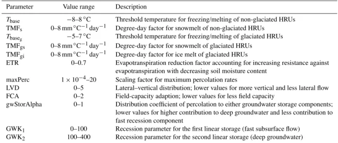
Table 1.Model calibration parameters and their value range. Parameterisation values apply to all HRUs unless specified differently.
Parameter Value range Description
Tbase −8–8◦C Threshold temperature for freezing/melting of non-glaciated HRUs
TMFs 0–8 mm◦C−1day−1 Degree-day factor for snowmelt of non-glaciated HRUs
Tbaseg −5–7
◦C Threshold temperature for freezing/melting of glaciated HRUs
TMFgs 0–8 mm◦C−1day−1 Degree-day factor for snowmelt of glaciated HRUs
TMFgi 0–8 mm◦C−1day−1 Degree-day factor for ice melt of glaciated HRUs
ETR 0–0.7 Evapotranspiration reduction factor accounting for increasing resistance against
evapotranspiration with decreasing soil moisture content maxPerc 1×10⁻⁴–20 Scaling factor for maximum percolation rates
LVD 0–5 Lateral–vertical distribution; lower values for more vertical and less lateral flow
FCA 0–2 Field-capacity adaption; lower values for less field capacity
gwStorAlpha 0–1 Distribution coefficient of percolation to either groundwater storage components; lower values for higher contribution to deep groundwater and less contribution to fast recession component
GWK1 0–100 Recession parameter for the first linear storage (fast subsurface flow)
GWK2 100–400 Recession parameter for the second linear storage (deep groundwater)
of precipitation provided as rain or snow is based on a thresh-old value, Tbase, which is determined in the calibration
pro-cess. Snow and ice melt are calculated using a degree-day method based on time-degree factors (TMFs) according to
melt[mm day−1] =TMF×(Tair−Tbase), (1)
whereTairis the air temperature. A total of three TMFs are
introduced in the model: one for snow of regular HRUs, i.e. non-glaciated HRUs; one for snow of glacier HRUs (see Sect. 4.1.3); and one for ice of glacier HRUs. Meltwater orig-inating from snow and ice of glacier HRUs is considered as glacier meltwater Qglac. Glacier mass balance is calculated
as the difference of glacier HRUs’ precipitation input and the sum of glacier HRUs’ snow and ice melt (i.e. Qglac), as well as actET. We introduce two independent TMFs for snow because of several dependencies that we can scarcely assess. These include increases in TMF with increasing so-lar radiation and elevation, and with decreasing proportions of sensible heat flux and albedo (Hock, 2003). Furthermore, we cannot validate at high elevation the temperature data sets used. Hence, this approach provides a more detailed analysis of effects of individual data sets. Glaciers in J2000g have no defined volume and could theoretically melt or store infinite amounts of water. While this does not, of course, represent the actual conditions, it allows for comparison of overesti-mating and underestioveresti-mating precipitation data sets due to the compensation of the water balance by means of increased glacier runoff. Meltwater and liquid precipitation are trans-ferred to the soil water module, which consists of a sim-ple water storage with a capacity (calibration factor FCA) derived from the field capacity of individual HRUs. Water stored in the soil, within the range of the storage capacity, can only leave through evapotranspiration. The calculated actual evapotranspiration (actET) depends on the saturation of the soil water storage, the potET, and a calibration parameter,
ETR. The soil storage must be saturated before runoff gener-ation can start. The amount of water exceeding the soil water storage is distributed into a lateral and a vertical component, based on the HRU’s slope and the calibration factor LVD (lateral–vertical distribution). The vertical component is con-sidered as percolation and is transferred to the groundwa-ter storage component. The maximum amount of percolation is limited by the calibration parameter maxPerc. Base flow
Qbas is simulated with a linear outflow routine adjusted by
the recession parameter GWK (groundwater turnover time), which is defined as
GWK[days] = V
Q, (2)
whereV is the storage volume in mm, andQis the outflow from this storage in mm day−1. The lateral excess water is di-rect runoffQdirwithout retardation. J2000g’s soil module
to the groundwater module in its design, J2000g treats both components as groundwater storages, and hence we use the termsQbas1andQbas2for the resulting discharge from these
components. Percolation water is distributed into the two lin-ear storage components based on the distribution coefficient gwStorAlpha. Finally,Qdirand the twoQbascomponents of
each HRU are summed up to give the total simulated stream-flowQtot.
J2000g does not have water routing through individual HRUs in a topological context like more complex models, such as J2000. As a result, the J2000g model cannot ac-count for losses and transformations during runoff concen-tration. We accept this limitation due to insufficient informa-tion available about soil and hydrogeological properties and assumed quick runoff on steep slopes without complex re-infiltration processes between HRUs.
4 Data
We use HRUs based on raster cells. All needed parameters were processed in the R environment (R Core Team, 2014) and finalised using open-source GIS software (GRASS-GIS and QGIS). We use a spatial resolution of 0.01◦ to balance the computational expense vs. the resolving power of some data sets. Linkage of the meteorological raster data to the single HRUs was achieved by overlay. The static parameters are considered constant over the time of the study and are provided once. The model runs with a daily temporal reso-lution. Meteorological data were either directly provided at daily resolution or downscaled if they provided a higher res-olution. The parameter and meteorological input data used in this work are described in the following two sections. An overview of these data, as well as their spatial and temporal resolution, is given in Table 2.
4.1 Geographical model parameters
4.1.1 Elevation, slope, and aspect
Elevation is taken from an SRTM (Shuttle Radar Topogra-phy Mission) DEM (digital elevation model) (Jarvis et al., 2008) with 90 m resolution (http://srtm.csi.cgiar.org). Slope and aspect are derived from this DEM with GIS software.
4.1.2 Soil
Soil data are taken from the Harmonized World Soil Database (HWSD) (FAO et al., 2009) and from the Atlas of the Republic of Tajikistan (Narzikulov and Stanjukoviˇc, 1968). A combination of the HWSD database and the clas-sification from the atlas that referred to soils by occurrence (e.g. alpine meadow or high-mountain desert) was used to parameterise the soil map. Leptosoils are the predominant soils. The HWSD provides grain size distributions for the first 30 cm for all leptosoil subtypes, and depths from 30 to
100 cm for most others. To derive the field capacities that represent a parameter of the J2000g model, empirical ta-bles of the soil mapping manual Bodenkundliche Kartier-anleitung (KA5) (Ad-hoc-Arbeitsgruppe Boden, 2005) were used. First, the bulk density given by the HWSD was used to derive the dry density (Ad-hoc-Arbeitsgruppe Boden, 2005, p. 126). Then the soil type was determined by using a soil type diagram (Ad-hoc-Arbeitsgruppe Boden, 2005, p. 142), in which the grain size distributions were used to derive the according soil types. The field capacities were derived as a function of soil type and dry density (Ad-hoc-Arbeitsgruppe Boden, 2005, p. 344). In combination with the information from the HWSD, the depth of the soils in cm and the total water capacity in mm were extracted. We assume vertical ho-mogeneity of all soils for the parameterisation of soil water capacity.
4.1.3 Land use and glacier extent
For land use, we extract the IGBP (International Geosphere-Biosphere Programme) classification scheme, included in the combined MODIS data set MCD12Q1 (Strahler et al., 1999). We use the 2005 classification, which marks the middle of the investigation period. The Gunt and Shakhdara catchments are sparsely vegetated by xeromorphic dwarf shrubs. Casual field observations in August 2011 have shown that vegetation diversity and vegetation cover are low along the main stem of the Gunt River. Vanselow and Samimi (2014) used a satellite-imagery-based approach to model vegetated land cover in the eastern Pamirs (Murghab and Alichur). They estimated half of the region to have<15 % vegetated land cover, which in-cludes the extensive alpine meadows in the vicinity of the main stem of the rivers. We observed only closed vegeta-tion cover at these spatially limited alpine meadows on the plateau, in the eastern part of the catchment (≈3800 m a.s.l.). In combination with the long-lasting snow cover, we assume vegetation to have only a minor impact on the overall water balance.
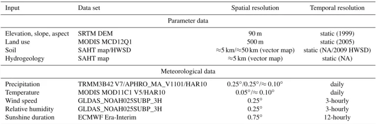
Table 2.Input used for derivation of HRUs and meteorological input data with specifications about temporal and spatial resolution. For static parameters the date of creation is given if available. SAHT is the State Administration for Hydrometeorology of Tajikistan and HWSD is the Harmonized World Soil Database. Resolutions of digitised SAHT and HWSD maps that are in vector format are roughly approximated. For the actual modelling, hourly values were averaged or summed up to yield daily values.
Input Data set Spatial resolution Temporal resolution
Parameter data
Elevation, slope, aspect SRTM DEM 90 m static (1999)
Land use MODIS MCD12Q1 500 m static (2005)
Soil SAHT map/HWSD ≈5 km/≈50 km (vector map) static (NA/2009 HWSD)
Hydrogeology SAHT map ≈5 km (vector map) static (NA)
Meteorological data
Precipitation TRMM3B42 V7/APHRO_MA_V1101/HAR10 0.25◦/0.25◦/≈0.10◦ daily
Temperature MODIS MOD11C1 V5/HAR10 0.05◦/≈0.10◦ daily
Wind speed GLDAS_NOAH025SUBP_3H 0.25◦ 3-hourly
Relative humidity GLDAS_NOAH025SUBP_3H 0.25◦ 3-hourly
Sunshine duration ECMWF Era-Interim 0.75◦ 12-hourly
(1978) and Breckle and Wucherer (2006). The according plant characteristics are then taken from the online database PlaPaDa (Plant Parameter Data) (Breuer and Frede, 2003). These characteristics comprise values for albedo, stomata re-sistances, leaf area indices, plant heights, and root depths. For the different seasonal and monthly characteristics, the as-sumption was made that little to no plant transpiration would take place during the long-lasting snow cover from autumn to spring (Immerzeel et al., 2009). To simulate this effect, the stomata resistance values were increased from November to March.
4.1.4 Hydrogeology
Hydrogeological information was taken from the Atlas of the Republic of Tajikistan (Narzikulov and Stanjukoviˇc, 1968). The study area comprises five lithologies and two other classes – one for ice/snow and one for lakes. The ice/snow extent differed from the land cover classification. Therefore we reclassified mismatching areas for snow/ice in the hy-drogeological map according to nearest-neighbour adjacent lithologies. At this stage, we have no quantitative hydro-geological information and rely on some literature values (Batu, 1998) and assign maximum percolation rates between 20 mm day−1 for magmatic rocks (including fractured rock
aquifers) and 300 mm day−1for Quaternary sediments.
Dur-ing the optimisation process, J2000g calibrates the correction factor maxPerc.
4.2 Meteorological data
4.2.1 Precipitation
Based on the work of Palazzi et al. (2013) and Ménégoz et al. (2013), who both emphasise radical differences in
precipita-tion data sets from various sources in the high mountains of Asia, we include a total of three precipitation data sets, one remote sensing product, one interpolated data set, and one climate model data set in order to assess their influence on the representation of the hydrological cycle. Evaluation of the data sets by comparison with in situ data is impeded by the point-wise character of rain/snow gauges on the one hand and area-averaged values of the raster data on the other (Tustison et al., 2001). Precipitation events taking place near the rain gauge might contribute to the data set but are not recorded for the in situ measurement. A moving rainstorm might also introduce a temporal error, because it will be recorded only within a restricted time frame at the measuring station. Fur-thermore, meteorological stations are located in the valleys. Hence, they cannot record advective precipitation at high al-titude. Different spatial resolutions of the data sets used com-plicate a representative analysis even more. Correlation anal-yses carried out with in situ data, consequently, show no sig-nificant correlation on a daily basis. If intensities are added up to monthly values (Fig. 5), correlation increases, espe-cially for the higher resolution data set. The differences in the data sets and few in situ data prevent an in-depth evalua-tion.
● ● ● ● ● ● ● ● ● ● ● ● ● ● ● ● ● ● ● ● ● ● ● ● ● ● ● ● ● ● ● ● ● ● ● ● ● ● ● ● ● ● ● ● ● ● ● ●
10 20 30 40 50 60
0 10 20 30 40 50
TRMM3B42 V7 [mm/month]
in situ [mm/month]
y = 0.44 x + 7.2 R²=0.26
● ● ● ● ● ● ● ● ●● ● ● ● ● ● ● ● ● ● ● ● ● ● ● ● ● ● ● ● ● ● ● ● ● ● ● ● ● ● ● ● ● ●● ● ● ● ●
0 50 100 150
0 10 20 30 40 50 HAR10 [mm/month]
in situ [mm/month]
y = 0.22 x + 1.8 R²=0.7
● ● ● ● ● ● ● ● ● ● ● ● Jan Feb Mar Apr May Jun Jul Aug Sep Oct Nov Dec ● ● ● ● ● ● ●● ● ● ● ● ● ● ● ● ● ● ● ● ● ● ● ● ● ● ● ● ● ● ● ● ● ● ● ● ● ● ● ● ● ● ●● ● ● ● ●
0 10 20 30 40 50
0 10 20 30 40 50 APHRO_MA_V1101 [mm/month]
in situ [mm/month]
y = 0.68 x + 9.76 R²=0.21
Figure 5. Comparison of precipitation data sets with in situ data on a monthly scale. Colour code for months indicates systematic under- and overestimations for TRMM3B42 V7 and APHRO_MA_V1101. The grey-shaded area marks 95 % modelled confidence inter-val. TRMM3B42 V7 and APHRO_MA_V1101 show the largest scatter. APHRO_MA_V1101 shows a large negative bias in winter and positive bias in summer. HAR10 has the highest correlation coefficient, but it has a major bias.
Table 3.Precipitation data sets with applied correction factors (CF). APHRO is APHRO_MA_V1101, and TRMM is TRMM3B42 V7. Values inside parentheses correspond to the resulting average an-nual precipitation amount that an individual data set provides after the application of the correction factor.
Data set name Correction CF for downscaled
factor (CF) HAR10 (CF∗)
APHRO (152 mm) 1.00 –
APHRO (200 mm) 1.30 –
TRMM (308 mm) 1.00 –
TRMM (400 mm) 1.30 –
HAR10 (172 mm)∗ 0.25 1.00
HAR10 (224 mm)∗ 0.32 1.30
HAR10 (258 mm)∗ 0.37 1.50
∗Note that HAR10 in its original version provides 688 mm of average
annual precipitation and has been downscaled in a first step to yield a ratio of unity with in situ measurements. This was done based on the mean of all meteorological stations and the mean of all pixels encompassing these stations (the resulting data set is HAR10 (172 mm)). The correction factors stated for HAR10 data sets in the third column were applied after this correction. Resulting overall CFs for HAR10 based on the uncorrected data set are according to CF=CF∗/4.05. (see Fig. 6b and Sect. 4.2.1 for an explanation).
several reasons. The most important one is to test the sen-sitivity of the models to precipitation. Second, the compar-ison of point measurements (in situ data) with gridded data sets (area-integrated values) is biased (Tustison et al., 2001). Third, we have no possibility to assess local precipitation lapse rates (different to the west–east gradient) or methods to infer orographic shielding that could, for example, result in a wet windward and a dry leeward region. Depending on the location of a meteorological station, this can already result in a significant bias between gridded and in situ data. Lastly, there are no validation data for glacier melt. This results in two unknowns – real precipitation amount and real glacier melt contribution toQtot. Hence, overestimation
(underesti-mation) of either quantity can be compensated for by under-estimation (overunder-estimation) of the other. Therefore, the eval-uation of applied correction factors will be discussed based on the modelled representation of the hydrograph during the snowmelt and glacier melt period, and based on an intercom-parison of obtained model results with different forcing data sets.
The TRMM (Tropical Rainfall Measuring Mission) Multi-satellite Precipitation Analysis (TMPA) product TRMM3B42 V7 (Huffman, 1997; Huffman et al., 1997, 2007) was chosen as the remote sensing product due to its frequent use along the Himalayan front (Bookhagen and Bur-bank, 2010; Roe, 2005; Kamal-Heikman et al., 2007). The 3B42 algorithm uses a two-step approach to compute precip-itation distribution. In the first step, TRMM’s Visible and In-frared Scanner (VIRS), TRMM Microwave Imager (TMI) or-bit data, and TMI/TRMM Combined Instrument (TCI) cali-bration parameters produce monthly infrared (IR) calicali-bration parameters. In the second step, these calibration parameters are then used to adjust merged-IR precipitation data of sev-eral geostationary satellites to derive 3-hourly and daily (de-rived from the 3-hourly) accumulated precipitation data at 0.25◦×0.25◦spatial resolution with full longitudinal cover-age. The data are validated with selected ground-truth infor-mation. The newest version (V7) includes additional sources of passive microwave satellite precipitation over the previous version (V6).
is of special interest for the study area because low precipi-tation amounts are recorded at the two highest sprecipi-tations, and because low temperatures suggest most of the precipitation to fall as snow. Detection problems of falling snow related to already existent snow cover have been pointed out by, for example, Yin (2004). Even though microwave imagers as used for the TRMM3B42 product can recognise snowfall, the quality relies on the discrimination between frozen pre-cipitation and antecedent snow cover (Skofronick-Jackson and Weinman, 2004). Other authors have reported an un-derestimation of precipitation in cases of intense snowfall in the Himalayas (Kamal-Heikman et al., 2007). Our anal-ysis of TRMM3B42 V7 data shows data records in winter, when precipitation must fall as snow. These data records show single precipitation events rather than a constant sig-nal that could be expected if the sigsig-nal was the result of the snow cover (which is persistent throughout the winter). We simply cannot assess the accuracy of TRMM3B42 V7 inten-sities at this point, but we chose this product to have a re-motely sensed product for our approach. To assess its quality performance, we independently applied an interpolated and a climate model data set for validation.
The interpolated data set is the APHRODITE (Asian Pre-cipitation Highly Resolved Observational Data Integration Towards Evaluation of Water Resources) monsoon Asia ver-sion 11, APHRO_MA_V1101 (Yatagai et al., 2009, 2012). The monsoon Asia region with a spatial coverage of 15◦S– 55◦N and 60–155◦E and a temporal coverage from 1951 to 2007 with daily temporal resolution was used. The prod-uct is a weighted interpolation prodprod-uct of ground-based pre-cipitation gauge data. The weighting is based on horizon-tal distance and an orographic correction model. Andermann et al. (2011) demonstrated that APHRODITE monsoon Asia V1003R1 is the best-performing precipitation data set avail-able for the central Himalayas, and the successor data set, APHRO_MA_V1101, has also been applied for Himalayan-wide glacier melt studies (Lutz et al., 2014).
The third data set is that of the High Asia Reanalysis (Maussion et al., 2014). The data result from a dynam-ical downscaling of global analysis data (Final Analysis data from the Global Forecasting System (National Cen-ters for Environmental Prediction, NOAA, US Department of Commerce, 2000; data set ds083.2) using the Weather Research and Forecasting (WRF-ARW) model (Skamarock and Klemp, 2008). Hence the quality of HAR depends on the global analysis data used as initialisation, as well as the model’s capability to simulate the atmospheric processes. Maussion et al. (2011) have shown good correlation of HAR with rain gauge data despite occasional overestimation on the Tibetan Plateau. Hence, HAR is assumed to show a good rep-resentation of seasonal patterns, however with the limitation of the need to calibrate precipitation intensities. From the dif-ferent spatial resolutions available (30 and 10 km), we use the 10 km version (HAR10) for precipitation without making use of the discriminated rain/snow parts, as we leave this to be the
subject of the model optimisation. Mölg et al. (2013) show that HAR10 shows good agreement with automatic weather stations on the Tibetan Plateau and therefore has high poten-tial for glacier studies.
Comparison of each data set with in situ data shows that differences in monthly added-up values for TRMM3B42 V7 and APHRO_MA_V1101 are relatively small compared to HAR10 (Fig. 6a). Seasonal biases are, however, very pro-nounced for all data sets. HAR10 shows high overestimations in winter. The ratio of an individual data set and in situ data (Fig. 6b) reveals that HAR10, despite overestimating, shows a constant ratio to in situ data, suggesting a rather systemati-cal error.
It should be noted that the obtained ratio is strongly biased by the included meteorological stations used in this compar-ison. Figure 6b shows, for example, that the individual re-sulting ratios of HAR10 with the two sites Navabad and Bu-lunkul differ by a factor of 3.5. As mentioned in Sect. 2, sta-tion Bulunkul is surrounded by mountain flanks that likely intercept incoming precipitation. This might lead to the pro-nounced overestimation of HAR10 in this situation.
APHRO_MA_V1101 and TRMM3B42 V7 show varying ratios but a lesser volume mismatch. If assuming positive precipitation lapse rates a grid value of either data set should overestimate observational data, because meteorological sta-tions are located on the valley floors. However, HAR10 pre-cipitation in its original version provided too much precipi-tation to the model, being unable to deal with resulting ex-tremely high snowmelt amounts. Based on that we correct HAR10 precipitation intensities downward to obtain a ra-tio with in situ data of 1. This downward correcra-tion at the beginning is only conducted for HAR10 because the other data sets were able to simulate the hydrograph. In a second step we apply correction factors to all precipitation data sets to account for possible positive precipitation lapse rates. We apply factors ranging from 1 to 1.5 (see Table 3) to the indi-vidual precipitation data sets. In the case of the downscaled HAR10 data set, the resulting overall factor with respect to the original data ranges from 0.25 to 0.37. Hereafter, we refer to the data sets according to their annual average precipita-tion amount, e.g. HAR10 (172 mm) for the HAR10 version with 172 mm average annual precipitation.
The precipitation data sets show different
spa-tial and seasonal distributions. TRMM3B42 V7 and
58.71
7.88 −5.26
−200
−100
0
100
200
Dataset − InSitu [mm/month]
2002 2003 2004 2005 2006
TRMM3B42V7
APHRO_V1101_MA
HAR10
over/under−prediction
1.41 4.05
9.34 (Bulunkul)
2.62
(Navabad)
0.73
0.1
0.5
5.0
50.0
Dataset / InSitu
2002 2003 2004 2005 2006
TRMM3B42V7
APHRO_V1101_MA
HAR10
ratio against in situ
A
B
Figure 6.Comparison of precipitation data sets with in situ data. Solid lines are mean monthly values for all pixels encompassing meteoro-logical stations. Dashed horizontal lines are mean values for the entire period from 2002 to 2006.(a)Difference in intensities on a monthly basis. There is strong overestimation for HAR10 and underestimation for TRMM3B42 V7 and APHRO_MA_V1101 in winter. Shaded area marks range between minimum and maximum of raster and in situ data.(b)Normalised data sets by in situ data show a constant value of≈4 for HAR10 and varying values for TRMM3B42 V7, and APHRO_MA_V1101 (extreme values in summer 2003 due to almost no recorded precipitation events in the in situ data set). Ratios of individual sites to a data set pixel encompassing this site can vary substantially (compare Navabad and Bulunkul). Different correction factors are applied to account for this uncertainty (see Sect. 4.2.1). Note the logarithmic scale.
Figure 7.Comparison of MODIS MOD11C1 V5 night LST and HAR10 2 m air temperature with in situ data. Scatter plots represent values for all pixels encompassing a meteorological station providing data. Scattering is actually smaller and correlation is higher when comparison is based on a single pixel and the encompassed meteorological station data. For calibration, the intercept values of the linear models with fixed slope of 1 (red) are added to the original data sets.
4.2.2 Temperature
We use two different data sets for air temperature – one de-rived from remote sensing data and one from a climate model data set. The data sets are calibrated based on available in situ data. Remote sensing determination of air temperature at ground level is not available at a global scale. Land surface temperatures (LSTs), on the other hand, can be determined from surface-emitted thermal infrared radiation, which can pass through the atmosphere. It can thus be measured with appropriate instruments from space. We correlate LSTs with in situ data to use them as a proxy for air temperatures.
The LST data set is the MODIS MOD11C1 V5 (Wan and Li, 1997; Wan et al., 2004; Wan, 2008) data that pro-vide night and daytime LST along with emissivity. The data are available as a 0.05◦×0.05◦resolution climate modelling
The climate model data set is the HAR10 2 m air temper-ature data. It is based on the same downscaling method used for HAR10 precipitation that was mentioned before. Due to HAR10’s reported usefulness for glacier balance studies (Mölg et al., 2013) and good representation of snow cover on the Tibetan Plateau (Maussion et al., 2011), along with a distinct correlation with in situ data (Fig. 7), we include this data set to see whether it provides a good all-in-one solution for the two key meteorological drivers. Correlation with in situ temperatures is expectedly lower compared to MODIS MOD11C1 V5, because of HAR10’s coarser spatial resolu-tion of 10 km, which averages values over a larger spatial domain.
Our comparison of LST with in situ air temperature shows high correlation (R2=0.83 for all pixels encompassing me-teorological stations) (Fig. 7). Pronounced underestimation for lower temperatures reduces the overall slope. This leads to an increased underestimation for higher temperatures. Therefore, we apply a linear regression with a fixed slope of one (linear model 1) to have a more representative depen-dency for the more important higher temperatures (affecting freezing, melting, and evapotranspiration). Based on the re-gression analysis, we calibrate the LST data set to match the observed air temperatures from the meteorological stations. Comparison of HAR10 and in situ data show a similar char-acteristic, and hence we apply the same correction procedure.
4.2.3 Wind speed and relative humidity
Wind speed and relative humidity data are based on the Noah land surface model (Chen and Dudhia, 2001; Chen et al., 2007; Ek et al., 2003) from the Global Land Data Assimilation System (GLDAS) (Rodell et al., 2004). We use the GLDAS_NOAH025SUBP_3H (Hydrological Sciences Branch at NASA/Goddard Space Flight Cen-ter , GSFC/HSB) data set provided in 3-hourly temporal and 0.25◦×0.25◦ spatial resolution. The data basis com-prises various satellite and in situ data (for more informa-tion see http://mirador.gsfc.nasa.gov/collecinforma-tions/GLDAS_ NOAH025SUBP_3H__001.shtml).
The extracted 3-hourly wind speed data were aver-aged to daily data. For relative humidity, further calcula-tions had to be performed as GLDAS_NOAH025SUBP_3H only provides specific humidity. Water vapour and at-mospheric pressures are needed to calculate relative hu-midity from specific huhu-midity (Häckel, 1999). However, GLDAS_NOAH025SUBP_3H does not provide vapour pressure. Therefore, relative humidity was calculated based on information provided by the LP DAAC (Land Processes Distributed Active Archive Center) (see Appendix A).
4.2.4 Sunshine duration
For sunshine duration, coarse (0.75◦×0.75◦) ECMWF (Eu-ropean Centre for Medium-Range Weather Forecast)
Interim data were obtained from ECMWF servers. ERA-Interim data incorporate modelled climate data from a wide range of satellite and in situ measurements (Dee et al., 2011). Sunshine duration is demanded by the model internal calcu-lation of global radiation . It serves as a proxy for cloudiness to reduce the internally calculated extraterrestrial radiation.
5 Model calibration
The JAMS framework utilises the Shuffled Complex Evolu-tion method of the University of Arizona (SCE-UA) (Duan et al., 1994), which is efficiently approaching an optimal set of model calibration parameters in an iterative process (Fis-cher et al., 2009). A set of given values for the calibration parameters will result in a certain realisation of a chosen ef-ficiency criterion. All possible realisations will span a sur-face in an+1 dimensional space, where n is the number of calibration parameters. The SCE-UA algorithm searches for the optimal calibration that is given by the global maxi-mum or minimaxi-mum (depending on whether the efficiency cri-terion has to be maximised or minimised) of this surface. The term “shuffled complex” derives from multiple sets of points (complexes) that are used to approach the extrema. The points that belong to a complex are shuffled every itera-tion (evoluitera-tion), enabling the algorithm to search the surface in a very efficient way, as has been shown by Duan et al. (1994). The Nash–Sutcliffe efficiency (NSE) (Nash and Sut-cliffe, 1970) was chosen as the efficiency criterion.
The NSE calculation is based on modelled and measured daily discharge measurements for Khorog (see Sect. 2). The same SCE optimisation procedure is conducted for all model setups. We always add an additional 300 mm to a each pre-cipitation data set at the beginning of the modelling pe-riod to account for empty groundwater storages and snow stocks. For the earlier-starting setups with temperature from MOD11C1 V5 this is on 1 March 2000, and for the setups with HAR10 temperature it is on 1 January 2001. The spin-up phase ends on 1 January 2002. Similar baseflow and snow stock values for the models with different temperature data suggest sufficient spin-up time for the setups with HAR10 that only have a 1-year spin-up phase. The actual calibration is then restricted to the period from 2002 to 2007. Due to the short period of available in situ data and high interannual variability in observed discharge, we use all available data for calibration and do not carry out an additional validation period. Instead, we address observed differences of individ-ual modelled years to point out differences in forcing data and their effect on the hydrological cycle.
6 Results
0
5
10
15
sno
wmelt [mm/d]
70
60
50
40
30
20
10
0
precipitation [mm/d]
0
1
2
3
4
5
6
Q_bas
, Q_glac [mm/d]
−20
0
20
T [°C]
0
100
200
SWE [mm]
base flow(Q_bas) snowmelt
precipitation glacier runoff(Q_glac)
snow water eq. temperature
0
1
2
3
4
5
6
Q_tot [mm/d]
0
5
10
15
20
Q_tot_cum
ulativ
e [km³]
2002 2003 2004 2005 2006 2007
observed
observed_cumulative TRMM3B42V7 308mm APHRO1101 200mm HAR10 258mm
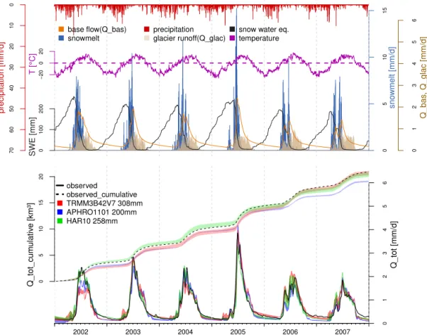
Figure 8.J2000g modelling results. Upper panel shows the individual water components for the overall best-performing model setup with MOD11C1 V5 temperature and HAR10 (258 mm). Note different scaling forQbas/Qglaccompared to snowmelt, due to higher magnitude of
snowmelt. Lower panel shows observed and modelled hydrographs and cumulative hydrographs. Displayed range (shaded area) corresponds to different temperature data sets.
amount of groundwater discharge and a transition from snow into glacier melt during summer. Strongest differences were apparent if significantly different amounts of winter precipi-tation were provided. The fact that cold temperatures during winter prevented any liquid precipitation and snow or glacier melt caused a strong constraint on the parameterisation of the groundwater aquifer. Low winter precipitation resulted in in-creased glacier melt and vice versa. Modelled variabilities in the well-pronounced intra-annual cycle were consistent be-tween different models and independent of the precipitation data set used. This highlights the temporal decoupling of pre-cipitation and discharge, and a strong influence of tempera-ture on the modelling.
6.1 Modelling results
Best NSE and lowest RMSE (root-mean-squared error) were obtained using a combination of MOD11C1 V5 temperature and HAR10 (258 mm) precipitation (Table 1). Setups with MOD11C1 V5 temperature consistently resulted in better NSE and 7–15 % smaller RMSE than setups with HAR10 temperature. The hydrological cycle according to the best
obtained model results is shown in Figs. 8 and 9 and can be summarised as follows: starting at the end of autumn, all precipitation is accumulated as snow cover. During this time
Qtotresults entirely fromQbas. In April, the melting season
starts with high peak discharges and replenishment of the groundwater reservoir. Snow stocks rapidly decline between April and July (Fig. 9a). During the middle of the melting season (July, August) snowmelt transitions into glacier melt. Finally, at the end of summer, there is no snow cover left and glacier melt is the only meltwater component. At this time,Qtotconsists mainly of groundwater discharge and, to a lesser extent, glacier melt (Fig. 9b). Then the cycle starts again. Because glacier melt directly becomes Qdir in the
model, it cannot infiltrate into soils and storage components. As a result, only snowmelt and rainfall contribute to ground-water replenishment. Glacier melt is the only effective sur-face runoff component during late summer. actET correlates with snowmelt and shows highest values in the narrow period from May to July, peaking in June with values of 1 mm day−1
1.5
1.0
0.5
0.0
precipitation, actET [mm/da
y]
J F M A M J J A S O N D
0
1
2
3
4
melt [mm/da
y]
−20
−10
0
10
20
temper
ature [°C]
0
50
100
150
200
SWE [mm]
precipitation actET temperature snow water eq. snowmelt Qglac
J F M A M J J A S O N D
0.0
0.5
1.0
1.5
2.0
Q [mm/d]
Qglac(ice) Qglac(snow) Qbas1 Qbas2
B
A
Figure 9.Monthly average hydrometeorological components(a)and hydrograph with discharge components(b)based on modelling results from 2002 to 2007 for the best-performing setup with HAR10 (258 mm) precipitation and MOD11C1 V5 temperature.
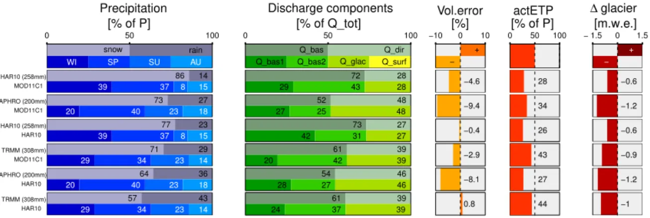
snow rain
WI SP SU AU
0 50 100
[% of P] Precipitation
Q_bas Q_dir Q_bas1 Q_bas2 Q_glac Q_surf 0 50 100
[% of Q_tot] Discharge components
+ − −10 0 10
[%] Vol.error
0 50 100
[% of P] actETP
+ −
− 1.5 0 1.5
[m.w.e.] ∆ glacier
MOD11C1
HAR10 (258mm) 86 14
39 37 8 15
72 28
29 43 28 −4.6 28 −0.6
MOD11C1
APHRO (200mm) 73 27
20 40 23 18
52 48
27 25 48 −9.4 34 −1.2
HAR10
HAR10 (258mm) 77 23
39 37 8 15
73 27
42 31 27 −0.4 26 −0.6
MOD11C1
TRMM (308mm) 71 29
29 34 23 14
61 39
20 42 39 −2.9 43 −0.9
HAR10
APHRO (200mm) 64 36
20 40 23 18
54 46
28 27 46 −8.1 27 −1.2
HAR10
TRMM (308mm) 57 43
29 34 23 14
61 39
24 37 39 0.8 44 −1
Figure 10.Average annual/intra-annual model results for the two different temperature data sets in combination with the individual best-performing precipitation data set. Descending ordering according to best NSE. The first panel is the legend. All discharge components as percent of average annualQtot. Negligible amounts ofQsurfresult from the model’s treatment of snowmelt water with a recession, which is
therefore represented byQbas1(see Sect. 3.2).
Smallest deviations for cumulative discharge were ob-served for models with precipitation from HAR10 (258 mm). For setups with TRMM (308 mm), a higher underesti-mation in 2002 and 2004, when SWE values were also much smaller, compared to HAR10 (258 mm) and APHRO (200 mm) was observed. Use of APHRO (200 mm) resulted in the highest underestimation, which is most pronounced in winter. Higher glacier melt in summer for setups with APHRODITE_MA_V1101 precipitation reduced this under-estimation in summer. The higher fraction of summer precip-itation for TRMM3B42 V7 and APHRODITE_MA_V1101 was accompanied by a higher contribution of glacier runoff to total discharge and more negative glacier mass balances (Fig. 10). All models showed highest deviations from ob-served discharge in 2006 and 2007, which might be related to the mentioned lake level regulations. We could not verify this assumption.
Comparison of the best individual model setups regarding their inputs and outputs is presented in Fig. 10. The best mod-els showed a higher fraction of snowfall over rainfall. A
par-ticular precipitation data set showed higher snowfall propor-tions (≈10 %) with MOD11C1 V5 temperatures compared to HAR10 temperatures. Despite the big differences in snow fraction, values forQbas1(resulting from snowmelt) showed
comparable results of≈20–30 % ofQtot. An exception was
the model using the combination of HAR10 temperature and HAR10 (258 mm) precipitation with 42 %Qbas1. This was
accompanied with the longest recession coefficient for the fast recession subsurface flow (GWK1) of≈38 days. Other models with HAR10 temperature show values for GWK1 be-tween 14 and 30 days and models with MODIS temperature show values between 10 and 19 days (Table 4). Despite this deviation, and despite the difference between the proportions ofQbas1toQbas2for either temperature data set, all models
showed high consistency for (1) the sum ofQbas1andQbas2,
(2) the ratio ofQbasoverQdir, (3) the proportion ofQglacto
Qtot, and (4) the glacier mass balances. Only actET and the
volume errors showed noticeable differences.
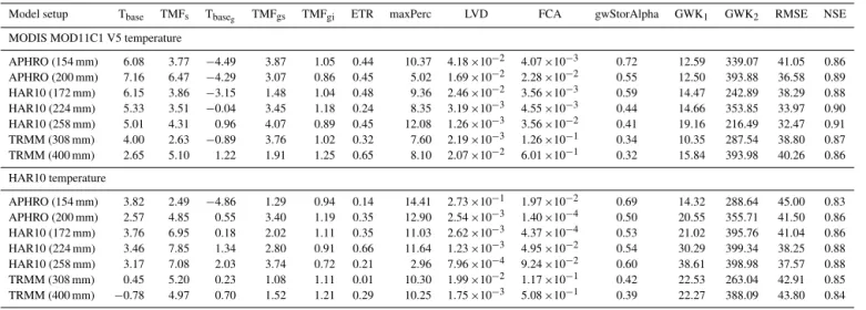
Table 4.Model parameterisations and NSE for the calibration time period 2002 to 2007.
Model setup Tbase TMFs Tbaseg TMFgs TMFgi ETR maxPerc LVD FCA gwStorAlpha GWK1 GWK2 RMSE NSE
MODIS MOD11C1 V5 temperature
APHRO (154 mm) 6.08 3.77 −4.49 3.87 1.05 0.44 10.37 4.18×10⁻² 4.07×10⁻³ 0.72 12.59 339.07 41.05 0.86
APHRO (200 mm) 7.16 6.47 −4.29 3.07 0.86 0.45 5.02 1.69×10⁻² 2.28×10⁻² 0.55 12.50 393.88 36.58 0.89
HAR10 (172 mm) 6.15 3.86 −3.15 1.48 1.04 0.48 9.36 2.46×10⁻² 3.56×10⁻³ 0.59 14.47 242.89 38.29 0.88
HAR10 (224 mm) 5.33 3.51 −0.04 3.45 1.18 0.24 8.35 3.19×10⁻³ 4.55×10⁻³ 0.44 14.66 353.85 33.97 0.90
HAR10 (258 mm) 5.01 4.31 0.96 4.07 0.89 0.45 12.08 1.26×10⁻³ 3.56×10⁻² 0.41 19.16 216.49 32.47 0.91
TRMM (308 mm) 4.00 2.63 −0.89 3.76 1.02 0.32 7.60 2.19×10⁻³ 1.26×10⁻¹ 0.34 10.35 287.54 38.80 0.87
TRMM (400 mm) 2.65 5.10 1.22 1.91 1.25 0.65 8.10 2.07×10⁻² 6.01×10⁻¹ 0.32 15.84 393.98 40.26 0.86
HAR10 temperature
APHRO (154 mm) 3.82 2.49 −4.86 1.29 0.94 0.14 14.41 2.73×10⁻¹ 1.97×10⁻² 0.69 14.32 288.64 45.00 0.83
APHRO (200 mm) 2.57 4.85 0.55 3.40 1.19 0.35 12.90 2.54×10⁻³ 1.40×10⁻⁴ 0.50 20.55 355.71 41.50 0.86
HAR10 (172 mm) 3.76 6.95 0.18 2.02 1.11 0.35 11.03 2.62×10⁻³ 4.37×10⁻⁴ 0.53 21.02 395.76 41.04 0.86
HAR10 (224 mm) 3.46 7.85 1.34 2.80 0.91 0.66 11.64 1.23×10⁻³ 4.95×10⁻² 0.54 30.29 399.34 38.25 0.88
HAR10 (258 mm) 3.17 7.08 2.03 3.74 0.72 0.21 2.96 7.96×10⁻⁴ 9.24×10⁻² 0.60 38.61 398.98 37.57 0.88
TRMM (308 mm) 0.45 5.20 0.23 1.08 1.11 0.01 10.30 1.99×10⁻² 1.17×10⁻¹ 0.42 22.53 263.04 42.91 0.85
TRMM (400 mm) −0.78 4.97 0.70 1.52 1.21 0.29 10.25 1.75×10⁻³ 5.08×10⁻¹ 0.39 22.27 388.09 43.80 0.84
model setups using only HAR10 data and the models us-ing APHRO (200 mm) (Fig. 10). Glacier mass balances show a factor of 2 difference. Smallest losses of−0.6 m w.e.yr−1
were obtained with HAR10 (258 mm). Highest losses of −1.2 m w.e.yr−1 were obtained with APHRO (200 mm),
which also showed the strongest negative volume errors of ≈ −9 % and substantially higher Qglac. Since this
in-dicates a strong underestimation of the already upward-corrected APHRO (200 mm) data set, we do not think that obtained model results of APHRO (200 mm) are represen-tative of the hydrological cycle.Qglac makes up≈30 % of
annual Qtot with HAR10 (258 mm) and up to 40 % with
TRMM (308 mm). The apparent higher glacier contribution for TRMM (308 mm) – despite providing more annual pre-cipitation – is compensated for by increased actET and is due to a higher portion of summer precipitation compared to HAR10 (258 mm).
6.2 Sensitivity analysis
Our sensitivity analysis is based on the convergence or non-convergence of calibration parameters and their value range obtained with the SCE-UA method with NSE as the opti-misation criterion. Three groups of parameters can gener-ally be differentiated. These groups are the ones determining (1) snowmelt, (2) glacier melt, and (3) groundwater proper-ties. At the beginning of the hydrological cycle, the snowmelt parameters dominate the representation of the hydrograph because snowmelt is the main contributor to river discharge. Then, depending on how much snow remains, glacier melt will start. Lastly, depending on when and how much wa-ter is available by means of snowmelt, respective groundwa-ter paramegroundwa-ters have to ensure that the wagroundwa-ter release is cor-rectly retarded and adjusted. The total amount of precipita-tion amassed as snow during the winter will thus represent the most important factor for the parameterisation.
We used a set of 12 calibration parameters (Table 1) and 8 complexes in the SCE-UA optimisation. Parameter values converged after 4000–5000 runs and showed no more than 1 % improvement in NSE later on. With limited information about specific soil and aquifer properties, all related soil and groundwater parameters were included in the SCE-UA opti-misation process. Wide value ranges for the calibration pa-rameters allowed for possible equifinality. Figure 11 shows the parameter calibration for both temperature data sets in-dependently. The best parameterisation as well as the value ranges for the individual best-performing precipitation data sets is highlighted. When considering all of the applied tem-perature and precipitation data sets, the most restricted pa-rameters were TMFgi and LVD, followed by Tbase, FCA,
and Tbaseg. The most unrestricted parameters were the
groundwater and the fast linear storage-component-related parameters GWK2, gwStorAlpha, maxPerc, and GWK1. In addition to these, TMF and ETR appear to be unrestricted. Constraints for a certain parameter were largely independent of the temperature data set used.
The degree-day factor for glacier melt TMFgi always
showed a narrow value range of about 1 mm◦C−1day−1.
Degree-day factors for snow were less constrained. The most obvious difference regarding the use of a specific tempera-ture data set were observed for the obtained threshold tem-peratures Tbase. Tbase for models with MOD11C1 V5 was about 2–3◦C higher than for models with HAR10 temper-ature. The threshold temperature for glaciers, Tbaseg, did
not show such a distinction between the different tempera-ture data sets. Low-precipitation-volume data sets, such as APHRO (154 and 200 mm) and HAR10 (172 mm), led to lowest Tbasegvalues in the setups with MOD11C1 V5. No
MOD11C1V5 0.92 0.7 20 1 100 2 5 8 7 8 8 8 410 NSE ETR maxPerc gwStorAlpha GWK2 GWK1 FCA LVD Tbase Tbase_g TMF_s TMF_gs TMF_gi PrecSum ● ● ● ● ● ● ● ● ● ● ● ● ● ● ● ● ● ● ● ● ● ● ● ● ● ● ● ● ● ● ● ● ● ● ● ● ● ● ● ● ● ● ● ● ● ● ● ● ● ● ● ● ● ● ● ● ● ● ● ● ● ● ● ● ● ● ● ● ● ● ● ● ● ● ● ● ● ● ● ● ● ● ● ● 400 ● ● ● ● ● ● ● ● ● ● ● ● ● ● ● ● ● ● ● ● ●● ● ● ● ● ● ● ● ● ● ● ● ● ●● ● ● ● ● ● ● TRMM3B42V7 308mm APHRO1101 200mm HAR10 258mm HAR10 0.92 0.7 20 1 100 2 5 8 7 8 8 8 410 NSE ETR maxPerc gwStorAlpha GWK2 GWK1 FCA LVD Tbase Tbase_g TMF_s TMF_gs TMF_gi PrecSum ● ● ● ● ● ● ● ● ● ● ● ● ● ● ● ● ● ● ● ● ● ● ● ● ● ● ● ● ● ● ● ● ● ● ● ● ● ● ● ● ● ● ● ● ● ● ● ● ● ● ● ● ● ● ● ● ● ● ● ● ● ● ● ● ● ● ● ● ● ● ● ● ● ● ● ● ● ● ● ● ● ● ● ● 400 ● ● ● ● ● ● ● ● ● ● ● ● ● ● ● ● ● ● ● ● ●● ● ● ● ● ● ● ● ● ● ● ● ● ● ● ● ● ● ● ● ● TRMM3B42V7 308mm APHRO1101 200mm HAR10 258mm -8 0 0 0 100 1E-040.82 -5 0 0 0 0 0 0
Figure 11. Ranges (shaded areas) for calibration parameters during the last steps of SCE-UA optimisation. Only parameterisations for NSE≥0.82 are considered. Possible value ranges are according to Table 1. The left panel displays realisations with setups using MOD11C1 V5 temperatures, and the right panel shows those with HAR10 temperatures. Solid lines represent best-performing individual precipitation data sets. PrecSum is the average annual precipitation.
Figure 12.Area-normalised discharge (specific discharge) dependencies on area-normalised precipitation (specific precipitation) and specific effective precipitationPeff, i.e. all liquid water input from rainfall, snowmelt (SM), and glacier melt (GM). All plots except for(f)are on a bi-logarithmic scale. Modelled discharge (MOD11C1 V5 temperature and HAR10 (258 mm) precipitation) response to(a)precipitation and(b)Peff. Colour-coding corresponds to month of the year. Error bars represent 95th percentiles and numbers represent mean monthly values. Panels(d)and(e)include model results from all other model combinations (shaded area) showing the same relationships as(a)and
(b), respectively; colour coding corresponds to precipitation data sets. Best individual precipitation data sets with either temperature data set are represented by the solid or dashed lines. Panel(c)shows for comparison purposes the discharge–rainfall relationship for the Naryani catchment, central Himalayas, Nepal. The shape is included in(d)and(e)to highlight similarity in shape but different order of magnitude in both discharge and precipitation. Panel(f)displays modelled discharge–temperature relationship.
store very little water and distribute the majority of this wa-ter to the underlying storage components. For the setups with