Study of Singularities in Nonsmooth Dynamical Systems via Singular Perturbation∗
Jaume Llibre†, Paulo R. da Silva‡, and Marco A. Teixeira§
Abstract. In this article we describe some qualitative and geometric aspects of nonsmooth dynamical systems theory around typical singularities. We also establish an interaction between nonsmooth systems and geometric singular perturbation theory. Such systems are represented by discontinuous vector fields onRℓ,ℓ≥2, where their discontinuity set is a codimension one algebraic variety. By means of a regularization process proceeded by a blow-up technique we are able to bring about some results that bridge the space between discontinuous systems and singularly perturbed smooth systems. We also present an analysis of a subclass of discontinuous vector fields that present transient behavior in the 2-dimensional case, and we dedicate a section to providing sufficient conditions in order for our systems to have local asymptotic stability.
Key words. regularization, vector fields, singular perturbation, discontinuous vector fields, sliding vector fields
AMS subject classifications. 34C20, 34C26, 34D15, 34H05
DOI. 10.1137/080722886
1. Introduction. The purpose of this article is to present some aspects of the geometric theory of a class of nonsmooth systems. Our main concern is understanding the dynamics of such systems by means of tools in the geometric singular perturbation theory. Many similarities between such fields were observed, and a comparative study of the two categories is called for. The main task for the future is to bring the theory of nonsmooth dynamical systems to a maturity similar to that of smooth systems. Needless to say, geometric singular perturbation theory is an important tool in the field of continuous dynamical systems, of which very good surveys are available (see [6, 7, 9]). The techniques of geometric singular perturbation theory can be used to obtain information on the dynamics of the nonsmooth system, mainly in searching minimal sets.
The study of nonsmooth dynamical systems has in recent years established an important bridge between Mathematics, Physics, and Engineering. The book [5] presents motivating models that arise in the occurrence of impact motion in impact systems as well as switchings in electronic systems and hybrid dynamics in control systems. For a survey on qualitative
∗Received by the editors April 30, 2008; accepted for publication (in revised form) by H. Kokubu December 17, 2008; published electronically March 18, 2009.
http://www.siam.org/journals/siads/8-1/72288.html
†Departament de Matem`atiques, Universitat Aut`onoma de Barcelona, 08193 Bellaterra, Barcelona, Catalonia, Spain ([email protected]). This author was partially supported by MTM2005-06098-C02-01 and by CICYT grant 2005SGR 00550.
‡Departamento de Matem´atica, IBILCE–UNESP, Rua C. Colombo, 2265, CEP 15054–000 S. J. Rio Preto, S˜ao Paulo, Brazil ([email protected]). This author was partially supported by FAPESP, CNPq, CAPES, and FAPESP– BRAZIL grant 2007/06896-5.
§IMECC–UNICAMP, CEP 13081–970, Campinas, S˜ao Paulo, Brazil ([email protected]). This author was partially supported by FAPESP–BRAZIL grant 2007/06896-5.
aspects of such systems we refer the reader to [14] and references therein. In many appli-cations examples of nonsmooth systems where the discontinuities are located on algebraic varieties are available (see, for example, [1,2]). See, for instance, the system represented by ¨
x+xsign(x) +sign( ˙x) = 0. Concerning theoretical results on this subject we refer the reader to [3, 12]. This paper is mainly motivated by such issues. It is worthwhile to point out that in [4] and [10] preceding results were established in two dimensions and three dimensions, respectively, when the discontinuity set is a codimension one submanifold.
Let X be a nonsmooth vector field in Rl, and denote by S its discontinuity set. First we focus our attention on the flow (determined by the orbits of X tending toS) that is tangent to S, which is denominated the sliding mode. It appears when the flow of X across S and points “inward” cannot leave such a surface.
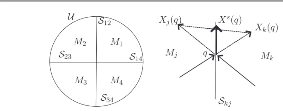
Now we address the discussion to a more general context. Let U ⊆Rℓ,ℓ≥2, be an open set with 0 ∈ U. Let S = S1S2, where S1 and S2 are codimension one submanifolds of U with 0∈ S1∩ S2 that are in general position. Around 0∈ U we have that S1∪ S2 separates U into four open quadrants: M1, . . . , M4. In our approachS will be the discontinuity boundary of our systems, also named the switching variety.
Let Xi, i = 1, . . . ,4, be Cκ vector fields, with κ 1, κ = ∞, or κ = ω, defined on
U. We are concerned with the behavior of the sliding mode generated from a discontinuous differential system expressed by
(1.1) z˙=X(z) =Xi(z), z∈Mi, i= 1, . . . ,4.
We will denote these systems byX = (X1, . . . , X4)∈Ωκ1234(U) and the intersectionMi∩Mj
by Sij.
Throughout the paper we consider local coordinates (x1, x2, . . . , xℓ) such thatS1 =S14∪ S23={x2 = 0},S2 =S12∪ S34={x1 = 0}, and
M1 ={x1>0, x2 >0}, M2 ={x1 <0, x2>0},
M3 ={x1<0, x2 <0}, M4 ={x1 >0, x2<0}.
Denote by S∗ = S \(S1 ∩ S2) the regular part of S. In S∗ the definition of an orbit-solution obeys, whenever possible, the Filippov convention (see [8]). Consider Mi and Mj,
i=j, having a common boundary. According to this convention there may exist generically a sliding regionSsl⊂ S∗ such that any orbit which meetsSslremains tangent toS∗for positive time. This region is the part of S∗ on which X
i and Xj point inward to S∗. Analogously
there may exist generically an escaping region Ses⊂ S∗ such that any orbit which meets Ses
remains tangent to S∗ for negative time.
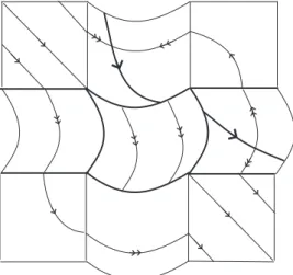
On SslSes the flow slides on S∗; the flow follows a well-defined vector field XS called the sliding vector field. See Figure 1. The sewing region Ssw ⊂ S∗ is the part of S∗ where the flow crosses S∗. The boundary between the three regions is the locus of points where the vector field is tangent to S∗ and the flow grazes the switching surface. In our context such points together with the critical points of XS and S
1∩ S2 constitute the set of singularities of X.
S14 S12
S23
S34 M1 M2
M3 M4
U
Skj
Mj q Mk
Xk(q)
Xj(q) Xs(q)
Figure 1. Boundary of four regions and the sliding vector field.
been the object of many studies. In the specific topic addressed in this paper the situation may be even more complicated since we want to study the dynamics of the vector field X around the origin. Alexander and Seidman in [1,2] established a discussion of such a situation by using two mechanisms termedblending and hysteresis. Our approach is closest in spirit to the works [4] and [10], and one of our concerns is to know when a sliding flow in S∗ can be continued until the intersection S1∩ S2. In addition, we also present some applications of the techniques developed in [4] and [10] for analyzing the behavior of the so-called transient flow around 0.
We begin by explaining the main concepts with a concrete example before discussing the general result of this setting.
Example. Consider U ⊆ R3, an open set with 0 ∈ U and X = (X1, . . . , X4) ∈Ωκ1234(U). We denote Xi = (fi, gi, hi),i= 1, . . . ,4. Suppose that f1<0,g1 <0; f2 >0,g2 <0; f3 >0, g3 >0; and f4<0,g4 >0. This means that all vector fields point inward to the intersecting switching curve Σ =S1∩ S2 ={(0,0, x3)}. It is natural to extend the definition of the sliding vector field to this set. A possible sliding vector field is a convex combination ofX1,X2,X3, and X4. We denote this combination by
XλΣ1,...,λ4 =λ1X1+· · ·+λ4X4,
i=4
i=1
λi= 1.
If
rank
⎡ ⎣
f1(0) f2(0) f3(0) f4(0) g1(0) g2(0) g3(0) g4(0)
1 1 1 1
⎤ ⎦= 3,
then there exists an open set 0∈ U ⊆R3 such that for any (0,0, x3)∈ U the set
λ∈R4;
i=4
i=1
λi= 1, XλΣ1,...,λ4(0,0, x3)∈Σ
is a nonempty set with dimension one in R4. Clearly we face here an ambiguity situation, and naturally some questions arise. For example, What is required to avoid such ambiguity?, or
Let X = (X1, . . . , X4) ∈Ωκ1234(U). Summarizing, in what follows we give a rough overall description of the main results of this paper.
(a) There exist four curves
{γi(ψ, x1, ρ) = 0}, {αi(θ, x2, ρ) = 0}, i= 1,2,
with θ, ψ ∈ [0, π], x1, x2 ∈ R, ρ ∈ Rℓ−2, and such that the sliding region SslSes on the regular part S∗ is homeomorphic to one of them. Moreover, the sliding vector field XS is topologically equivalent to one of the following reducing problems:
γi(ψ, x1, ρ) = 0, x˙1 =δi(ψ, x1, ρ), ρ˙=νi(ψ, x1, ρ)
or
αi(θ, x2, ρ) = 0, x˙2=βi(θ, x2, ρ), ρ˙=σi(θ, x2, ρ).
See Theorem 2.2(a), (b).
(b) For ℓ≥3 there exists a differential system
ζ(θ, ψ, ρ) = 0, ξ(θ, ψ, ρ) = 0, ρ′ =φ(θ, ψ, ρ),
which extends the concept of the Filippov system for the case S1∩ S2. See Theorem2.2(c). (c) For ℓ= 2,X1 =X3, andX2 =X4, the flow of the regular vector fields which approach X = (X1, X2, X1, X2) in the transient case is described. See Proposition 5.4.
2. Preliminaries and statement of results. In this section basic concepts and the main result of the paper are presented.
The sliding vector field XS is defined at q ∈ S
kj∩(SslSes) by XS(q) = m−q, with
m being the point where the segment joining q+Xk(q) andq+Xj(q) cuts Skj. In previous
works (see [4,10,11]) it was shown that ifp= (x1, . . . , xℓ)∈ S1∪ S2 andx21+x22 = 0, then the sliding vector field on a neighborhoodV ofp can be studied via singular perturbation theory. Suppose that p = (0, x2, . . . , xℓ) ∈ S12, X = X1 = (f1, g1) ∈ R ×Rℓ−1 if x1 > 0, X =X2 = (f2, g2)∈R×Rℓ−1 ifx1 <0, andf1(p)·f2(p)= 0.
Definition 2.1. A C∞-function ϕ : R −→ R is a transition function if ϕ(s) = −1 for
s−1, ϕ(s) = 1 ifs1, and ϕ′(s)>0 if s∈(−1,1).
The ϕx2-regularization of X is the one-parameter family given by
(2.1) Xε12= (1/2) [(1 +ϕ(x1/ε))X1+ (1−ϕ(x1/ε))X2]
forx2>0,ε >0.
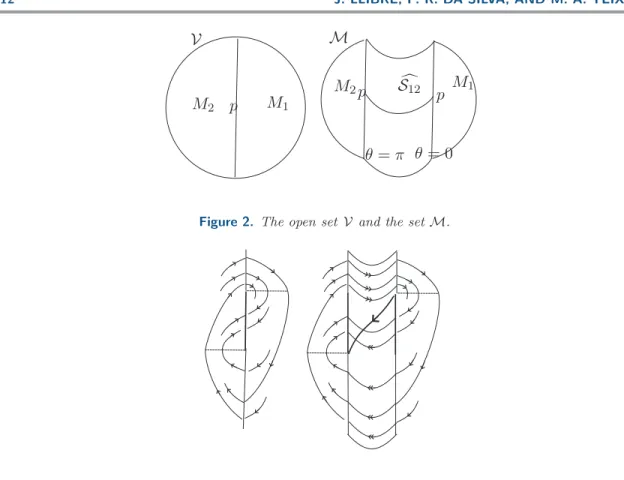
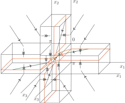
Consider, around the point p, the surface composed by the union of M1∩ V,M2∩ V, and
S12={(θ, ρ) :θ∈(0, π), ρ= (x2, . . . , xℓ)∈ S12∩V}. We denoteM= (M1∩V)∪S12∪(M2∩V) and remark that the set{(0, ρ) :ρ∈S12∩V}has two distinct copies: ∂(M1∩V) and∂(M2∩V). The blow-up process is the change of coordinates x1 = rcosθ, ε = rsinθ. It induces a smooth vector field on Mwhose trajectories coincide with those ofX1 onM1, of X2 on M2, and of a singular perturbation problem on S12 described by
M1 p
M2 V
S12 p M1 p
M2 M
θ= 0 θ=π
Figure 2. The open set V and the setM.
Figure 3. Fast and slow dynamics with the slow manifold connecting two folds.
with r ≥0, θ ∈(0, π), ρ∈ S12∩ V, and α and β of class Cκ. We remark that the functions α(r, θ, ρ) and β(r, θ, ρ) are given by
α=−sinθ
f1+f2
2 +ϕ(cotθ)
f1−f2 2
, β = g1+g2
2 +ϕ(cotθ)
g1−g2 2 ,
with the functionsfi, gi,i= 1,2, depending on (rcosθ, ρ). See Figures2and 3.
Clearly in a neighborhood of 0 ∈ Rℓ we have two singular perturbation problems, SP1 and SP2, defined on the sets r ≥ 0, θ ∈ (0, π) for ρ ∈ S12, and for ρ ∈ S34, respectively. Moreover, another two singular perturbation problems, SP3 and SP4, defined on the sets u≥0,ψ∈(0, π) forη ∈ S14, and forη ∈ S23, respectively, still occur. Our main result is the following.
Theorem 2.2. Consider X = (X1, . . . , X4)∈Ωκ1234(U). There exist a neighborhood V ⊆ U
of 0 and the following singular perturbation problems defined at 0∈Rℓ:
θ′=αi(r, θ, x2, ρ), x2′ =rβi(r, θ, x2, ρ), ρ′ =rσi(r, θ, x2, ρ), i= 1,2; (2.3)
ψ′=γi(u, ψ, x1, ρ), x1′=uδi(u, ψ, x1, ρ), ρ′ =uνi(u, ψ, x1, ρ), i= 1,2;
(2.4)
and
with r, u≥0, θ, ψ∈[0, π], (x1, x2, ρ)∈ V, ρ= (x3, . . . , xℓ). Moreover,αi, βi, σi, γi,δi,νi,ζ,
ξ, and φare of class Cκ for i= 1,2 and satisfying the following:
(a) The sliding region (SslSes)∩S1 is homeomorphic to the slow manifold {γi(0, ψ, x1, ρ)
= 0} \ Zψ ={ψ= 0, π} of (2.4), withi= 1 atS14 and with i= 2 atS23. The sliding
vector field XS is topologically equivalent to the reduced problem γ
i(0, ψ, x1, ρ) = 0,
˙
x1=δi(0, ψ, x1, ρ), and ρ˙=νi(0, ψ, x1, ρ).
(b) The sliding region (SslSes)∩S2 is homeomorphic to the slow manifold {αi(0, θ, x2, ρ)
= 0} \ Zθ ={θ = 0, π} of (2.3), with i= 1at S12 and with i= 2 at S34. The sliding
vector field XS is topologically equivalent to the reduced problem α
i(0, θ, x2, ρ) = 0,
˙
x2=βi(0, θ, x2, ρ), andρ˙=σi(0, θ, x2, ρ).
(c) The singular perturbation (2.5) is the blowing up of the regularization of the systems (2.3)fori= 1,2. The slow manifold is given bySM1={ζ(0,0, θ, ψ, ρ) = 0}.
Further-more, for ℓ≥ 3, the slow flow is the limit, for r, u ↓ 0, of the trajectories of another singular perturbation expressed by
(2.6) rθ˙=ξ(r, u, θ, ψ, ρ), ρ˙=φ(r, u, θ, ψ, ρ).
The slow manifold of (2.6) is the set on Rℓ given by
SM2 ={ξ(0,0, θ, ψ, ρ) = 0, ζ(0,0, θ, ψ, ρ) = 0} ⊆SM1.
In section 3 we focus on the concept of regularization discussed above, and we prove Theorem 2.2. The sets given byαi(0, θ, x2, ρ) = 0, γi(0, ψ, x1, ρ) = 0, and ζ(0,0, θ, ψ, ρ) = 0 are called slow manifolds, and they will be denoted by SM. We say that a slow manifold is nontrivial if it is not contained inZ ={θ= 0, π} ∪ {ψ= 0, π}.
p
M1
M1
OX ϕX1(t1, p)
ϕX1(t2, p)
OY
M2 M2
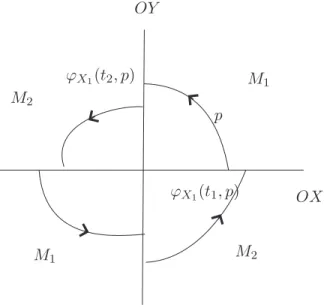
Figure 4. Transient vector fields around0.
conditions for the local asymptotic stability. Finally, in section5we study systems in this class that present a transient behavior. See section 5 for a precise definition. For an illustration see Figure4.
3. Proof of Theorem2.2. First we introduce some basic definitions. Consider a transition function ϕ.
(a) The ϕx2-regularization of X is the one-parameter family given by
(3.1) Xε12= (1/2) [(1 +ϕ(x1/ε))X1+ (1−ϕ(x1/ε))X2]
forx2>0,ε >0, and
(3.2) Xε43= (1/2) [(1 +ϕ(x1/ε))X4+ (1−ϕ(x1/ε))X3]
forx2<0,ε >0.
(b) The ϕx1-regularization of X is the one-parameter family given by
(3.3) Xa14= (1/2) [(1 +ϕ(x2/a))X1+ (1−ϕ(x2/a))X4]
forx1>0,a >0, and
(3.4) Xa23= (1/2) [(1 +ϕ(x2/a))X2+ (1−ϕ(x2/a))X3]
forx1<0,a >0. Denote
ϑ+ij = ϑi+ϑj 2 , ϑ
−
ij =
ϑi−ϑj
2 , λ(z) =ϕ(cot(z)), Sα =−sinα,
and
ϑ∗abcd⋆◦ = ϑa∗ϑb⋆ ϑc◦ϑd
4 ,
where ∗, ⋆,◦ ∈ {+,−}.
Let ϕ :R−→ Rbe a transition function. We remark that the mapping λ: [0, π] −→ R
given by λ(θ) =ϕ(cotθ) for 0< θ < π,λ(0) = 1, and λ(π) =−1 is a nonincreasing smooth function which is strictly decreasing for π4 < θ < 34π.
Proof of Theorem 2.2. For simplicity we suppose thatℓ= 3, and we writeXi = (fi, gi, hi),
i = 1, . . . ,4. Denote by Xr1, Xr2 the equations of (3.1) and (3.2), respectively, after the coordinate change ε=rsinθ,x1 =rcosθ. Let X1r and X2r be these equations after the time rescaling t = rτ. Let X3
r, Xr4 be the systems given by (3.3) and (3.4) now written in the
coordinates a = usinψ, x2 = ucosψ. Represent by X3r, X4r those systems after the time rescaling t = uτ. Thus Xr
i, i = 1,2, are the vector fields corresponding to the differential
systems (2.3), given in Theorem2.2, onS12and onS34, respectively. Analogously,Xir,i= 3,4,
are the vector fields corresponding to the differential systems (2.4), given in Theorem2.2, on
Table 1
The equations of the regularizations.
X1 r ⎧ ⎪ ⎨ ⎪ ⎩
rθ˙ = Sθ
f12+ +λ(θ)f − 12
˙
x2 = g12+ +λ(θ)g − 12
˙
x3 = h+12+λ(θ)h − 12 X2 r ⎧ ⎪ ⎨ ⎪ ⎩
rθ˙ = Sθ
f43++λ(θ)f − 43
˙
x2 = g43+ +λ(θ)g − 43
˙
x3 = h+43+λ(θ)h − 43 X3 r ⎧ ⎪ ⎨ ⎪ ⎩
uψ˙ = Sψ
g14+ +λ(ψ)g − 14
˙
x1 = f14+ +λ(ψ)f − 14
˙
x3 = h+14+λ(ψ)h − 14 X4 r ⎧ ⎪ ⎨ ⎪ ⎩
uψ˙ = Sψ
g23+ +λ(ψ)g − 23
˙
x1 = f23++λ(ψ)f − 23
˙
x3 = h+23+λ(ψ)h − 23 Xr 1 ⎧ ⎪ ⎨ ⎪ ⎩
θ′ = S
θ
f+
12+λ(θ)f − 12
x′ 2 = r
g+
12+λ(θ)g − 12
x′3 = r
h+
12+λ(θ)h − 12 X r 2 ⎧ ⎪ ⎨ ⎪ ⎩
θ′ = S
θ
f+
43+λ(θ)f − 43
x′ 2 = r
g+
43+λ(θ)g − 43
x′3 = r
h+
43+λ(θ)h − 43 Xr 3 ⎧ ⎪ ⎨ ⎪ ⎩
ψ′ = S
ψg+14+λ(ψ)g − 14
x′
1 = u
f+
14+λ(ψ)f − 14
x′3 = u
h+
14+λ(ψ)h − 14 X r 4 ⎧ ⎪ ⎨ ⎪ ⎩
ψ′ = S
ψg23+ +λ(ψ)g − 23
x′
1 = u
f+
23+λ(ψ)f − 23
x′3 = u
h+
23+λ(ψ)h − 23 1 3 2 4 0 3 4 0 0 0 1 2 0 0 0 X X X X X X X X X ψ π π θ
Figure 5. Local vector fields in the blowing-up locus.
Since the proofs of the cases (a) and (b) are similar, we will prove only (b) for x2 > 0. The slow manifold for θ∈(0, π) is implicitly determined by the equation f12+ +λ(θ)f12− = 0. We have that f12− = 0 if and only iff1(0, x2, x3) =f2(0, x2, x3).
We denote f(x1, x2, x3) and f(r, θ, x2, x3) before and after the blow-up, respectively. If (0, θ, x2, x3)∈(SslSes), then the vector fields point inward or outward. This implies that
f1(0, θ, x2, x3).f2(0, θ, x2, x3)<0.
Thus we have that f12−(0, θ, x2, x3)= 0 for any θ∈(0, π), (0, x2, x3)∈(SslSes). Since
f12+
f12− =±1⇒f1.f2 = 0,
we have
−1<−f +
12(0, θ, x2, x3) f12−(0, θ, x2, x3)
for all (0, θ, x2, x3)∈(SslSes). Moreover, the inverse of the restrictionλ|(π
4, 3π
4) is increasing
on (−1,1), and the equation f12++λ(θ)f12− = 0 defines a continuous graphic contained in
(θ, x2, x3)|x2∈R, x3 ∈R, θ∈
π 4, 3π 4 .
In accordance with the definition ofXS, we have thatXS =X
1+k(X2−X1) withk∈Rsuch thatX1(x1, x2, x3) +k(X2−X1)(x1, x2, x3) = (0, y2, y3) for somey2, y3. Thus it is easy to see that XS is given by XS =0,f1g2−f2g1
f1−f2 ,
f1h2−f2h1 f1−f2
. The reduced problem is then represented
by ˙x2 =g12+ +λ(θ)g12−, ˙x3 =h+12+λ(θ)h−12 under the restriction λ(θ) =−
f12+ f12−
. Then we must
have ˙x2 = f1gf21−−ff22g1, ˙x3 = f1hf21−−ff22h1. It follows immediately that the flows of XS and the reduced problem are equivalent.
To prove case (c) we consider the ϕx1-regularization ofX r
1 andX2r:
(3.5) Xa1r,2r
⎧ ⎪ ⎨
⎪ ⎩
θ′ = S
θ
f1234++++λ(θ)f1243−+−+ϕ(x2/a)f1234+−−+ϕ(x2/a)λ(θ)f1243−−+
, x′
2 = r
g1234++++λ(θ)g1243−+−+ϕ(x2/a)g1234+−−+ϕ(x2/a)λ(θ)g1243−−+
, x′
3 = r
h1234++++λ(θ)h1243−+−+ϕ(x2/a)h+1234−−+ϕ(x2/a)λ(θ)h−−1243+
.
The equations of the equivalent system with a=usinψ,x2 =ucosψ are
(3.6) ⎧ ⎪ ⎨ ⎪ ⎩
θ′ = S
θf1234++++λ(θ)f1243−+−+λ(ψ)f1234+−−+λ(ψ)λ(θ)f1243−−+
,
uψ′ = rS
ψ
g1234++++λ(θ)g1243−+−+λ(ψ)g1234+−−+λ(ψ)λ(θ)g−−1243+, x′3 = rh+++1234 +λ(θ)h−1243+−+λ(ψ)h+1234−−+λ(ψ)λ(θ)h−−1243+.
By means of the time rescaling τ =us we get (keeping the notationθ′, ψ′, x′
3 for simplicity)
(3.7) ⎧ ⎪ ⎨ ⎪ ⎩
θ′ = uS
θf1234++++λ(θ)f1243−+−+λ(ψ)f1234+−−+λ(ψ)λ(θ)f1243−−+
, ψ′ = rS
ψ
g1234++++λ(θ)g1243−+−+λ(ψ)g+1234−−+λ(ψ)λ(θ)g1243−−+, x′
3 = r
h1234++++λ(θ)h1243−+−+λ(ψ)h+1234−−+λ(ψ)λ(θ)h−−1243+.
Thus we have
ξ(r, u, θ, ψ, x3) =Sθf1234++++λ(θ)f1243−+−+λ(ψ)f1234+−−+λ(ψ)λ(θ)f1243−−+
,
ζ(r, u, θ, ψ, x3) =Sψ
g1234++++λ(θ)g1243−+−+λ(ψ)g+1234−−+λ(ψ)λ(θ)g1243−−+,
and
φ(r, u, θ, ψ, x3) =h+++1234 +λ(θ)h−1243+−+λ(ψ)h+1234−−+λ(ψ)λ(θ)h−−1243+.
We define the slow system (u= 0 at (3.6)) and the fast system (divide byr andu= 0 at (3.7)) at (x1, x2, x3) = (0,0, x3), respectively, by
(3.8) X00S
⎧ ⎨
⎩
0 = Sψ
g1234++++λ(θ)g1243−+−+λ(ψ)g1234+−−+λ(ψ)λ(θ)g1243−−+,
θ′ = S
θf1234++++λ(θ)f1243−+−+λ(ψ)f1234+−−+λ(ψ)λ(θ)f1243−−+
, x′
and
(3.9) X00F
⎧ ⎨
⎩
ψ′ = S
ψ
g1234++++λ(θ)g1243−+−+λ(ψ)g1234+−−+λ(ψ)λ(θ)g−−1243+, θ′ = 0,
x′
3 = 0.
This finishes the proof.
Next the results of the theorem are illustrated.
Example 1. Consider X1(x1, x2) = (−1,−1), X2(x1, x2) = (2,−1), X3(x1, x2) = (4,5),
and X4(x1, x2) = (−2,3). The trajectories of X01 are the solutions of the reduced problem
Sθ 1
2 − 32λ(θ)
= 0, ˙x2 = −1, where Sθ = −sinθ. The slow manifold is the curve θ = θ0
with λ(θ0) = 1/3, and the slow flow points to region x2 <0. The fast vector field is (θ′,0)
with θ′ <0 for θ > θ0 and θ′ >0 for θ < θ0. The trajectories of X02 are the solutions of the
reduced problem Sθ(1−3λ(θ)) = 0, ˙x2 = 4−λ(θ). The slow manifold is the curve θ = θ0
with λ(θ0) = 1/3, and since 4−λ(θ)>0 forθ∈(0, π), the slow flow points to region x2 >0.
The fast vector field is (θ′,0) withθ′ <0 forθ > θ0 and θ′ >0 forθ < θ0. The trajectories of X03 are the solutions of the reduced problemSψ(1−2λ(ψ)) = 0, ˙x1=−32+12λ(ψ). The slow
manifold is the curve ψ=ψ0 withλ(ψ0) = 1/2, and since ˙x1<0 forψ∈(0, π), the slow flow
points to region x1 <0. The fast vector field is (ψ′,0) withψ′ >0 for ψ < ψ0 and ψ′ <0 for ψ > ψ0. The trajectories of X04 are the solutions of the reduced problem Sψ(2−3λ(ψ)) = 0,
˙
x1= 3−λ(ψ). The slow manifold is the curve ψ=ψ1 withλ(ψ1) = 2/3, and since ˙x1 >0 for ψ ∈(0, π), the slow flow points to region x1 >0. The fast vector field is (ψ′,0) with ψ′ >0 for ψ < ψ1 and ψ′ <0 for ψ > ψ1. The trajectories of X00 are the solutions of the reduced
problem Sψ32 −12λ(θ)−52λ(ψ) + 12λ(ψ)λ(θ)= 0,θ′ =Sθ34 −92λ(θ)−14λ(ψ) + 34λ(ψ)λ(θ). The slow manifold is the curve 32−12λ(θ)−52λ(ψ) +12λ(ψ)λ(θ) = 0, which connects the points (θ, ψ) = (0, ψ0) and (θ, ψ) = (π, ψ1) with λ(ψ0) = 1/2 and λ(ψ1) = 2/3. In fact, if θ = 0,
then λ(θ) = 1, and 32 − 12λ(θ)− 52λ(ψ) + 12λ(ψ)λ(θ) = 0 implies λ(ψ) = 12, and if θ = π, then λ(θ) = −1, and 32 − 12λ(θ)− 52λ(ψ) + 12λ(ψ)λ(θ) = 0 implies λ(ψ) = 23. Observe that
3
2 − 12λ(θ)− 52λ(ψ) +12λ(ψ)λ(θ) = 0 implies θ′ =
Sθ
4(λ(θ)−5)(−15λ2(θ) + 83λ(θ)−12). There
exists a uniqueα= 8330−301 √6169∈(−1,1) such that−15α2+ 83α−12 = 0. Furthermore, if λ < α, then−15λ2+ 83λ−12<0, and if λ > α, then−15λ2+ 83λ−12>0. So there exists a uniqueθ∗∈(π4,34π) such thatλ(θ∗) =α and
0< θ < θ∗⇒λ(θ)> λ(θ∗)⇒θ′ >0
and
θ > θ∗ ⇒λ(θ)< λ(θ∗)⇒θ′<0.
Moreover, λ(θ0) = 1/3 and θ′>0 imply that θ0 < θ∗. See Figure 6.
Example 2. Consider X1(x, y) = (−y, x) and X2(x, y) = (1,−1). The trajectories of X01
are the solutions of the reduced problem −y+ 1
2 +λ(θ)
−y−1
2 = 0, y˙=− 1
2(1−λ(θ)).
The slow manifold is the curve y=y(θ) given byy= 1+1−λλ((θθ)). This function is increasing:
lim θ−→π
4
y(θ) = 0, lim θ−→3π
4
Figure 6. Local vector fields in the blowing-up locus of Example1.
Since 1−λ(θ)≥0, we have that ˙y≤0. So the slow flow points to region y <0. Denote θ(y) the inverse function of y(θ). The fast vector field is (θ′,0) with θ′ <0 forθ(y) < θ < π and
θ′>0 for 0< θ < θ(y). The trajectories of X02 are the solutions of the reduced problem
−y+ 1
2 +λ(θ)
y+ 1
2 = 0, y˙=− 1
2(1 +λ(θ)).
The slow manifold is the empty set. In fact, the right-hand side ofy = −1+λ(λθ()+1θ) is positive for
θ∈(π4,34π), and here we have y <0. The fast vector field is (θ′,0) with θ′<0 for 0< θ < π. The trajectories of X03 are the solutions of the reduced problem
x−1
2 +λ(ψ)
x+ 1
2 = 0, x˙ = 1
2(1−λ(ψ)).
The slow manifold is the curve x=x(ψ) given by x= 1+1−λλ((ψψ)). This function is increasing:
lim ψ−→π
4
x(ψ) = 0, lim ψ−→3π
4
x(ψ) = +∞.
We have ˙x≥0. So the slow flow points to region x >0. Denote byψ(x) the inverse function of x(ψ). The fast vector field is (ψ′,0) with ψ′ < 0 for 0 < ψ < ψ(x) and ψ′ > 0 for
ψ(x)< ψ < π. The trajectories ofX04 are the solutions of the reduced problem
x−1
2 +λ(ψ)
−x−1
2 = 0, x˙ = 1
2(1 +λ(ψ)).
The slow manifold is the empty set. In fact, the right-hand side of x= −1+λ(λψ()+1ψ) is positive, and here we have x < 0. The fast vector field is (ψ′,0) with ψ′ < 0 for 0 < ψ < π. The trajectories of X00 are the solutions of the reduced problem
−1
2 +λ(ψ)λ(θ) 1
2 = 0, θ ′= Sθ
The slow manifold is given by the equation λ(ψ)λ(θ) = 1, and the slow flow is θ′ = 0, which is highly degenerated. The fast vector field is (ψ′,0) with ψ′ ≤0 for 0 < ψ < π. Note that
λ(ψ)λ(θ) = 1 for all (θ, ψ)∈([0, π/4]×[0, π/4])∪([3π/4, π]×[3π/4, π]). See Figure7.
Figure 7. Local vector fields in the blowing-up locus of Example2.
4. Intersecting switching surfaces on R3
. In this section we consider the caseℓ= 3. We provide sufficient conditions in order for an equilibrium point of the reduced problem (2.6) to be a local attractor. See previous results in this direction in [12,13].
In what follows we use the notation
∂(Φ,Ψ) ∂(a, b) =
Φaa Ψab
Φba Ψbb
.
Proposition 4.1. Consider U ⊆ R3, an open set with 0 ∈ U and X = (X1, . . . , X4) ∈
Ωκ1234(U). Denote Xi = (fi, gi, hi), i = 1, . . . ,4. Let ζ, ψ be the functions which satisfy
ζ =Sθζ and ξ=Sψξ with ζ, ξ, and φgiven by (2.5). Let D⊆(0, π)×(0, π)×R be an open
neighborhood of (θ0, ψ0,0). Suppose that ζ(0,0, θ0, ψ0,0) =ξ(0,0, θ0, ψ0,0) = 0 and that for
(θ, ψ, x3)∈D we have
∂(ζ, ξ)
∂(θ, ψ) >0,
∂(ζ, ξ)
∂(θ, x3)
<0, ∂(ζ, ξ) ∂(ψ, x3)
<0.
Then the slow manifold SM2 is a curve parameterized by (θ(x3), ψ(x3), x3). Moreover, if
φ(θ0, ψ0,0) = 0, ∂ ∂x3
φ(θ0, ψ0,0)<0,
then (θ0, ψ0,0) is an attracting singular point of the reduced system (2.6).
Proof. It is enough to apply the implicit function theorem. The assertions about the singular point follow the fact that the reduced problem isx′
Example. Consider X = (X1, . . . , X4) ∈ Ωκ1234(U) given by X1 = (−1,−1,−x3), X2 = (2,−3,−x3), X3 = (1,2,−x3), andX4 = (−3,1,−x3). System (2.5) takes the form
uψ′ = rSψ(−41 +14λ(θ)−74λ(ψ) + 34λ(ψ)λ(θ)), θ′ = S
θ(−14− 74λ(θ) +34λ(ψ) + 14λ(θ)λ(ψ)),
x′
3 = −rx3.
The slow manifold SM1 is given by −1 +λ(θ)−7λ(ψ) + 3λ(θ)λ(ψ) = 0. This is a surface parameterized by (θ, ψ(θ), x3) with θ ∈ [0, π]. Moreover, the curve (θ, ψ(θ)) is such that it connects (θ, ψ) = (0, π/2) to (π, ψ2) with λ(ψ2) = −1/5. The fast vector field is such that ψ′>0 on the upper side andψ′ <0 otherwise. The slow manifoldSM
2 is represented by
−1 +λ(θ)−7λ(ψ) + 3λ(θ)λ(ψ) = 0,
−1−7λ(θ) + 3λ(ψ) +λ(θ)λ(ψ) = 0.
This curve is parameterized by (θ0, ψ0, x3),x3 ∈R, withλ(ψ0) = 11−4 √
11
2 andλ(θ0) = 3−√11
2 .
Since x′
3 = −x3, the slow flow on SM2 has an attracting singular point at (θ0, ψ0,0). See Figure 8.
0 π
π
x1 x1 x2
x2
x3 x3
Figure 8. A sequence of slow manifoldsSM2⊆SM1.
5. Transient vector fields on R2
Figure 9. T-type singular points.
theCκ-topology. ConsiderX
1, X2 ∈ Cκ(U,R2). The idea is to study the following nonsmooth system in U:
(5.1) X(q) =
X1(q) = (f1(q), g1(q)) if F(q)>0, X2(q) = (f2(q), g2(q)) if F(q)<0.
The case (a) was treated in [11]. The case (b) can be seen as a particular case of the system studied above when ε = −1. In this case we will denote X = (X1, X2) ∈ Ωκ12(U). The case when ε= 1 does not deserve to be analyzed. We choose local coordinates such that M =F−1(0) = {xy = 0}. Thus M
1 = {x.y > 0} and M2 = {x.y < 0}. In what follows we denote by OXi(p) = {ϕXi(t, p), t∈R} the orbit of the vector field X
i,i= 1,2, through the
point p.
Definition 5.1. We say that X = (X1, X2) ∈ Ωκ12(U), U ⊆ R2, is a transient vector field
around 0 if, for all p= (x, y)∈Mi for some i= 1,2, there exist t1, t2 ∈R such that OXi(p) (i = 1 if xy > 0 or i = 2 if xy < 0) cuts 0X \ {0} and 0Y \ {0} transversally for t = t1
and t = t2, respectively. Moreover, t1t2 < 0, and for any t between t1 and t2 we have that ϕXi(t, p)∈Mi.
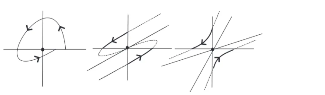
Definition 5.2. Let A∈M(2)be a 2×2real matrix. We say that (0,0) is a T-type singular point of A if the Jordan form of A, J(A), is one of the following.
• (focus-type) J(A) =β αα−β, with α·β = 0; • (improper node–type) J(A) = [α1
0 α], with α = 0 and with the eigenvectorω ∈Mi;
• (saddle- or node-type) J(A) = λ1 0
0 λ2
, with λ1 =λ2 ∈ R and with both eigenvectors
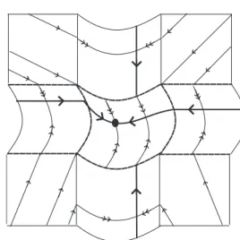
in the same Mi. See Figure 9.
Proposition 5.3. Let X= (X1, X2)∈Ω12κ (U), U ⊆R2, be a transient vector field. If (0,0)
is a hyperbolic singular point of Xi,i= 1,2, then (0,0) is a singular point of the linear vector
field DXi(0,0) of T type.
Proof. We have that (0,0) is a saddle or a node or a focus. The transient behavior of Xi implies that we cannot have orbits on Mi ∪ {(0,0)} with α-limit or ω-limit equal to
{(0,0)}.Moreover, if (0,0) is a saddle or a node, then the stable and unstable manifolds are on Mi∪ {(0,0)}.
Now we introduce some notation. Q1 ={(x, y);x >0, y >0}.
• We say thatXi fori= 1,2 is ofFij type in a neighborhood of (0,0) if (0,0) is a focus
or an improper node of Xi. Moreover, the trajectories are positively oriented ifj= 1
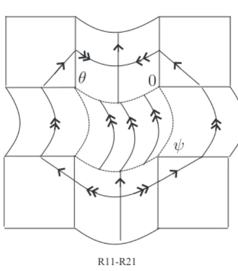
R11-R21
0 θ
ψ
Figure 10. Transient vector field of (R11, R21) type.
• We say that Xi for i = 1,2 is of Sij type in a neighborhood of (0,0) if (0,0) is a
saddle or a node of Xi and the trajectories onMi are positively oriented ifj= 1 and
negatively oriented ifj = 2.
• We say that X1 is of R1j type in a neighborhood of (0,0) if (0,0) is a regular point of
X1 andX1(0,0)∈Q2 if j= 1 and X1(0,0)∈Q4 ifj = 2.
• We say that X2 is of R2j type in a neighborhood of (0,0) if (0,0) is a regular point of
X2 andX2(0,0)∈Q1 if j= 1 and X1(0,0)∈Q3 ifj = 2.
• We say that (X1, X2) is of (A, B) type if X1 is ofA type andX2 is of B type.
Remark. We have 36 possible combinations for X1 and X2. However, we can reduce this number, observing that some cases can be identified by means of a rotation or a change of sign. For example, roughly speaking, (F12, F21) can be identified with −(F11, F22), and (S11, F21) can be identified with Rπ/2(F11, S21). Thus we have the following:
(a) If X1(0,0) ∈M2, X2(0,0) ∈M1, then, by means of a rotation, X = (X1, X2) is such that its phase portrait is of (R11, R21) type. See Figure 10.
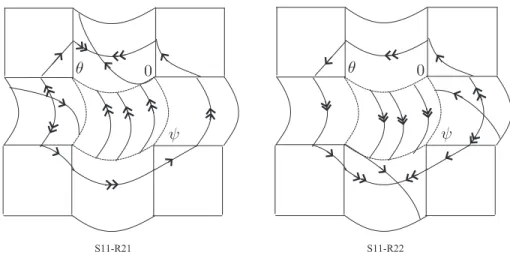
(b) If|X1(0,0)|.|X2(0,0)|= 0 and|X1(0,0)|2+|X2(0,0)|2 = 0, thenX = (X1, X2) is such that its phase portrait is of (F11, R21), (F11, R22), (S11, R21), or (S11, R22) type. See Figures11 and 12.
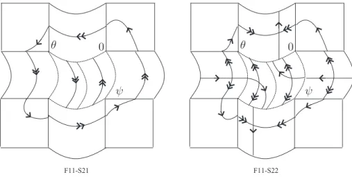
(c) If |X1(0,0)|2+|X2(0,0)|2 = 0, then X= (X1, X2) is such that its phase portrait is of (F11, F21), (F11, F22), (F11, S21), (F11, S22), (S11, S21), or (S11, S22) type. See Figures
13,14, and 15.
Example. Let X = (X1, X2) ∈ Ωk12(U) be a transient vector field defined on a neigh-borhood of 0 ∈ U ⊆ R2. Suppose that X1(0,0) = (a, b), ab < 0, and X2(0,0) = (c, d), with cd > 0. The slow manifold on the blowing-up locus corresponding to x1 > 0, x2 = 0 is Sψ(b+2d +b−2dλ(ψ)) = 0 and on the blowing-up locus corresponding to x1 < 0, x2 = 0 is Sψ(b+2d+d−2bλ(ψ)) = 0. If we considerbd <0, we have that−bb+−dd ∈(−1,1), which implies that
there exist ψ1, ψ2 ∈(π4,34π) such that the slow manifolds areψ=ψ1 andψ=ψ2, respectively. Finally, the equation of the slow manifold in the intersection is Sψ(b+2d+ b−2dλ(θ)λ(ψ)) = 0.
F11-R21
0 θ
ψ
F11-R22
0 θ
ψ
Figure 11. Transient vector fields of (F11, R21) type and (F11, R22)type.
S11-R21
0 θ
ψ
S11-R22
0 θ
ψ
Figure 12. Transient vector fields of (S11, R21) type and (S11, R22)type.
Proposition 5.4. LetX = (X1, X2)∈Ωk12(U) be a transient vector field defined on a
neigh-borhood of 0∈U ⊆R2. Denote
Ai =
ai −bi
bi ai
, i= 1,2,
Bλ =
sin(λ1+λ2) −2 cosλ1cosλ2
2 sinλ1sinλ2 −sin(λ1+λ2)
,
and
Cλ =
−2 sinλ1sinλ2 sin(λ1+λ2)
sin(λ1+λ2) −2 cosλ1cosλ2
.
F11-F21
0 θ
ψ
F11-F22
0 θ
ψ
Figure 13. Transient vector fields of (F11, F21) type and (F11, F22)type.
F11-S21
0 θ
ψ
F11-S22
0 θ
ψ
Figure 14. Transient vector fields of (F11, S21) type and (F11, S22)type.
and for b1 >0, b2 <0, and a1 =a2 the slow manifold is nontrivial and the slow flow
has a singular point.
(b) If X1(0,0) =X2(0,0) = (0,0), DX1(0,0) =A1, and b1 >0, 0< λ1< λ2 < π/2, then
forDX2(0,0) =Bλ the slow manifold is nontrivial and the reduced flow of system (2.5)
is singular; and forDX2(0,0) =−Bλ the slow manifold is nontrivial and the slow flow
has not only singular points. Moreover, if 2a1sin(λ1) sin(λ2) > b1sin(λ1+λ2), then
the slow flow has a singular point.
(c) If X1(0,0) = X2(0,0) = (0,0), DX1(0,0) = Cλ, 0 < λ1 < λ2 < π/2, and 0 < μ1 < μ2 < π/2, then forDX2(0,0) =Bµthe slow manifold is nontrivial and the reduced flow
of system (2.5) is singular; and for DX2(0,0) =−Bµ the slow manifold is nontrivial
and the slow flow has a part composed only of singular points and another part where there exists a singular point.
S11-S21
0 θ
ψ
S11-S22
0 θ
ψ
Figure 15. Transient vector fields of (S11, S21) type and (S11, S22)type.
focus type at (0,0), andBλ andCλ are the matrices of linear vector fields which have singular
points of saddle type at (0,0) with eigenvectors (cosλ1,sinλ1) and (cosλ2,sinλ2) in the first and second quadrants, respectively.
Proof of Proposition 5.4. Suppose that X1 and X2 satisfy the hypothesis of (a). The equation of the slow manifold is Sψ
2 cos(θ)((b1 +b2) + (b1−b2)λ(θ)λ(ψ)) = 0. If b1 >0 and b2 >0, then |bb11+−bb22|>1. This implies that the nontrivial part of the slow manifold is given by θ=π/2. Moreover, the slow flow is determined by θ′, which is zero for θ=π/2. If b1>0 and b2 <0, then|bb11−+bb22|<1, and thus (b1+b2) + (b1−b2)λ(θ)λ(ψ) = 0 defines two smooth
curves. The slow flow has a singular point because θ′ =S
θcos(θ)(a2−a1) has a sign change at θ= π2. So (a) is proved.
Suppose now that both X1 and X2 satisfy the hypothesis of (b). The equation of the slow manifold is Sψ
2 cos(θ)[(b1 + 2Sλ1Sλ2) + (b1 −2Sλ1Sλ2)λ(θ)λ(ψ)] = 0. If b1 > 0 and
0 < λ1 < λ2 < π/2, then Sλ1Sλ2 > 0. This implies that the nontrivial part of the slow
manifold is given by θ = π/2. Moreover, the slow flow is determined by θ′, which is zero for θ = π/2. If DX2(0,0) = −Bλ, then the slow manifold is S2ψ cos(θ)[(b1 −2Sλ1Sλ2) +
(b1+ 2Sλ1Sλ2)λ(θ)λ(ψ)] = 0. Since
b1−2Sλ1Sλ2 b1+2Sλ1Sλ2 ∈
(−1,1), the equation defines at least two
curves. The slow flow has a singular point because θ′ =S
θcos(θ)
2a1Sλ1Sλ2+b1Sλ1+λ2 b1+2Sλ1Sλ2
has a sign change at θ= π2. So (b) is proved.
Suppose now that X1 and X2 satisfy the hypothesis of (c). The equation of the slow manifold is Sψ
2 cos(θ)[(−Sλ1+λ2 + 2Sµ1Sµ2) + (−Sλ1+λ2−2Sµ1Sµ2)λ(θ)λ(ψ)] = 0. If 0< λ1 <
λ2 < π/2 and 0 < μ1 < μ2 < π/2, then −Sλ1+λ2 > 0 and Sµ1Sµ2 > 0. This implies that
the nontrivial part of the slow manifold is given by θ = π/2. Moreover, the slow flow is determined by θ′, which is zero for θ=π/2. If DX
2(0,0) =−Bµ, then the slow manifold is Sψ
2 cos(θ)[(−Sλ1+λ2−2Sµ1Sµ2) + (−Sλ1+λ2+ 2Sµ1Sµ2)λ(θ)λ(ψ)] = 0. Since
−Sλ1+λ2−2Sµ1Sµ2
−Sλ1+λ2+2Sµ1Sµ2 ∈
(−1,1), the equation defines at least two curves. The slow flow has a singular point because θ′ = S
θcos(θ)−8Sλ1Sλ−2SSλµ1Sµ2−2Sλ1+λ2Sµ1 +µ2 1+λ2+2Sµ1Sµ2
that if
δ = −8Sλ1Sλ2Sµ1Sµ2−2Sλ1+λ2Sµ1+µ2
−Sλ1+λ2 + 2Sµ1Sµ2
⇒sgn(δ) =−1,
then (c) is proved.
6. Conclusions. In this paper we propose a method of studying the dynamics around the intersection of codimension one discontinuity submanifolds. Using a regularization process proceeded by a blow-up, we get a singular perturbation problem. We also consider questions like transient behavior and asymptotic stability.
Acknowledgment. The authors express their gratitude to the referees for their helpful comments.
REFERENCES
[1] J. C. Alexander and T. I. Seidman, Sliding modes in intersecting switching surfaces. I. Blending, Houston J. Math., 24 (1998), pp. 545–569.
[2] J. C. Alexander and T. I. Seidman,Sliding modes in intersecting switching surfaces. II.Hysteresis, Houston J. Math., 25 (1999), pp. 185–211.
[3] M. Broucke, C. Pugh, and S. Simi´c,Structural stability of piecewise smooth systems, Comput. Appl. Math., 20 (2001), pp. 51–89.
[4] C. Buzzi, P. R. Silva, and M. A. Teixeira,A singular approach to discontinuous vector fields on the plane, J. Differential Equations, 231 (2006), pp. 633–655.
[5] M. di Bernardo, C. Budd, A. Champneys, and P. Kowalczyk,Piecewise-Smooth Dynamical Sys-tems. Theory and Applications, Appl. Math. Sci. 163, Springer-Verlag, London, 2008.
[6] F. Dumortier and R. Roussarie,Canard cycles and center manifolds, Mem. Amer. Math. Soc., 121 (1996), 132708.
[7] N. Fenichel,Geometric singular perturbation theory for ordinary differential equations, J. Differential Equations, 31 (1979), pp. 53–98.
[8] A. F. Filippov,Differential Equations with Discontinuous Righthand Sides, Math. Appl. (Soviet Ser.), Kluwer Academic Publishers, Dordrecht, The Netherlands, 1988.
[9] C. Jones,Geometric singular perturbation theory, in Dynamical Systems, C.I.M.E. Lectures (Montecatini Terme, 1994), Lecture Notes in Math. 1609, Springer-Verlag, Heidelberg, 1995, pp. 44–118.
[10] J. Llibre, P. R. Silva, and M. A. Teixeira,Regularization of discontinuous vector fields via singular perturbation, J. Dynam. Differential Equations, 19 (2007), pp. 309–331.
[11] J. Llibre, P. R. Silva, and M. A. Teixeira,Sliding vector fields via slow–fast systems, Bull. Belg. Math. Soc. Simon Stevin, 15 (2008), pp. 851–869.
[12] J. Llibre and M. A. Teixeira,Global asymptotic stability for a class of discontinuous vector fields in R2, Dyn. Syst., 22 (2007), 133–146.
[13] M. A. Teixeira,Stability conditions for discontinuous vector fields, J. Differential Equations, 88 (1990), pp. 15–29.