Abstract—The paper proposes a sequential computation method of the state vector associated to a circuit in dynamic behavior, for pre-established time intervals or punctually. Based on discrete circuit models with direct or iterative companion diagrams, the method is intended to a wide range of analog circuits: linear or nonlinear circuits, with or without magnetically coupled inductors or excess elements. The enclosed example proves the efficiency and the accessibility of the proposed analysis method.
Index Terms—Analog circuit, discrete modeling, numerical integration, state variable formulation.
I. INTRODUCTION
The discretization of the circuit elements, followed by corresponding companion diagrams, leads to discrete circuit models associated to the analyzed analog circuits [1,2]. Using the Euler, trapezoidal or Gear approximations [3,4], simple discretized models are generated, whose implementation leads to an auxiliary active resistive network. In this manner, the numerical computation of desired dynamic quantities becomes easier and faster. Considering the time constants of the circuit, the discretization time step can be adjusted for reaching the solution optimally, in terms of precision and computation time.
The discrete modeling of nonlinear circuits assumes an iterative process too, that requires updating the parameters of the companion diagram at each iteration and each integration time step [4,5]. If nonzero initial conditions exist, they are computed usually through a steady state analysis performed prior to the transient analysis.
The discrete modeling can be associated to the state variables approach [6,7], as well as the modified nodal approach [4,8], the analysis strategy being chosen in accordance with the circuit topology, the number of the energy storage circuit elements (capacitors and inductors) and the global size of the circuit.
The known computation algorithms based on the discrete modeling allow the sequential computation, step by step, along the whole analysis time, of the state vector or output vector directly [4,9]. In this paper, one proposes a method that allows computing the state vector punctually, at the moments considered significant for the dynamic evolution of the circuit. Thus, the sequential computation for pre-established time subdomains is allowed.
Manuscript received March 8, 2010.
The authors are with the University of Craiova, Romania, Faculty of Electrical Engineering, (phone/fax: +40-251-413102; e-mail: [email protected]).
II. MODELING THROUGH COMPANION DIAGRAMS The time domain analysis is performed for the time interval [t0,tf], bounded by the initial moment t0 and the final moment tf. It can be discretized with the constant time step h, chosen sufficiently small in order to allow using the Euler, trapezoidal or Gear numerical integration algorithms [1-4]. One can choose t0 =0 and tf =wh, where w is a positive integer.
The analog circuit analysis using discrete models requires replacing each circuit element through a proper model according to its constitutive equations. In this way, if the Euler approximation is used, the discretization equations and the corresponding discrete circuit models associated to the energy storage circuit elements are shown in table 1, for the time interval [nh,(n+1)h],h<w.
The tree capacitor voltages uC and the cotree inductor currents iL [6,7] are chosen as state quantities, assembled in the state vectorx. The currents
C
I of the tree capacitors and
the voltages across the cotree inductors UL are complementary variables, assembled in the vector X.
At the moment t=nh , the above named vectors are partitioned as:
=
n L n C n
i u
x ,
=
n L n C n
U I
X (1)
with obvious significances of the vectors Ln n C n L n
C i I U
u , , , .
For the magnetically coupled inductors, the discretized equations and the companion diagram are shown in table 1, where the following notations were used:
. ,
,
, ,
,
1 21 2 22 1 2 21 1 21 22 1 22
2 12 1 11 1 1 12 1 12 11 1 11
n n
n n
n
n n
n n
n
i h L i h L e h L R h L R
i h L i h L e h L R h L R
+ =
= =
+ =
= =
+ +
+
+ +
+
(2)
For nonlinear circuits, the state variable computation at the moment t=(n+1)h requires an iterative process that converges towards the exact solution [4,5]. A second upper index corresponds to the iteration order (see table 2). Similar results to those of table 1 and table 2 can be obtained using the trapezoidal [4,10] or Gear integration rule [3,4].
Punctual State Computation Using Discrete
Modeling
Table I: Discrete modeling of the energy storage elements.
No. Element Symbol Discretized expressions Companion diagram
1 Tree capacitor C I C u S C=1/
1
1 +
+ = + n
C n C n
C u hSI
u 1 + n C I hS 1 + n C u n C u
2 Excess capacitor C i C U S C=1/
(
n)
C n C n
C U U
hS i +1 = 1 +1−
1 + n C i hS 1 + n C U n C U hS 1
3 Cotree inductor
Γ =1/ L L U L i 1 1 +
+ = + Γ n
L n
L n
L i h U
i n L i Γ h 1 + n L U n L i
4 Excess inductor
Γ =1/ L
L
u
L
I
(
n)
L n L n
L I I
h
u −
Γ
= +
+1 1 1
1
+
n L
I 1/hΓ
n L I hΓ 1 1 + n L u 5 Magnetically coupled inductor pair 1 1 + n U * * 1 2 + n U 1 1 + n i 1 2 + n
i L12 L21
11 L 22 L 1 2 ' 1 ' 2 n n n n n n n n n n i R i R i R i R U i R i R i R i R U 2 22 1 2 22 1 21 1 1 21 1 2 2 12 1 2 12 1 11 1 1 11 1 1 − + + − = − + + − = + + + + + + 1 1 + n U 1 1+ n
i R11
1 2 ' 1 ' 2 1 1 + n
e 122+1
n i R 1 2 + n U 1 2 + n
i R22
1 2
+
n
e 211 1
+
n
i R
Table II: Iterative discrete modeling.
No. Element Iterative dynamic
parameter Companion diagram
Notations in the companion diagram 1 i u ) ( ˆ i u
u= i in m
m n i u R , 1 , 1 + = + ∂ ∂ = m n m n m n m n m n m n i R u e R R , 1 , 1 , 1 , 1 , 1 , 1 + + + + + + ⋅ − = = 2 i u q ) ( ˆ q u u= m n u u m n u q C , 1 , 1 + = + ∂ ∂ = m n m n m n m n m n m n i hS u e hS R , 1 , 1 , 1 , 1 , 1 , 1 + + + + + + ⋅ − = = 3 i u ϕ ) ( ˆ i ϕ
ϕ = i in m
m n i L , 1 , 1 + = + ∂ ∂ = ϕ 1 , 1 + + m n
i Rn+1,m m n e +1,
1 , 1 + + m n u m n m n m n m n m n m n i L h u e L h R , 1 , 1 , 1 , 1 , 1 , 1 1 1 + + + + + + ⋅ − = = 4 i u ) ( ˆu i
i= u un m
m n u i G , 1 , 1 + = + ∂ ∂ = m n m n m n m n m n m n u G i j G G , 1 , 1 , 1 , 1 , 1 , 1 + + + + + + ⋅ − = = 5 i u q ) ( ˆ u q q= m n q q m n q u S , 1 , 1 + = + ∂ ∂ = m n m n m n m n m n m n u C h i j C h G , 1 , 1 , 1 , 1 , 1 , 1 1 1 + + + + + + ⋅ − = = 6 i u ϕ ) ( ˆϕ i i= m n i m n , 1 , 1 + = + ∂ ∂ = Γ ϕ ϕ ϕ 1 , 1 + + m n i m n G +1,
m n j +1,
III. SEQUENTIAL AND PUNCTUAL STATE COMPUTATION The treatment with discretized models assumes substituting the circuit elements with companion diagrams, which consist in a resistive model diagram. It allows the sequential computation of the circuit solution.
A. Circuits without excess elements
If the given circuit does not contain capacitor loops nor inductor cutsets [6,7], the discretization expressions associated to the energy storage elements (table 1, lines 1 and 3), using the notations (1), one obtains
1
1 +
+
+
= n n
n x h S X
x
Γ 0
0
, (3)
where S is the diagonal matrix of capacitor elastances and Γ
is the matrix of inductor reciprocal inductances.
Starting from the companion resistive diagram, the complementary variables are obtained as output quantities [4,9,10] of the circuit
1
1 +
+ = n+ n
n Ex Fu
X , (4)
where E and F are transmittance matrices, and un+1 is the vector of input quantities [4,6,7] at the moment t=(n+1)h. From (3) and (4) one obtains an equation that allows computing the state vector sequentially, starting from its initial value x0 = x(0) until the final value xw= x(wh):
1
1 +
+ = n+ n
n M x Nu
x , (5)
where
E S
M
+ =
Γ 0
0
1 h , (6)
1 being the identity matrix, and
F S
N
=
Γ 0
0
h . (7)
Starting from eq. (5), through mathematical induction, the useful formula is obtained as
∑
= −
+
= n
i
k k n n
n
1
0 M Nu x
M
x , (8)
where the upper indexes of the matrix M are integer power exponents. The formula (8) allows the punctual computation of the state vector at any moment t=nh, if the initial conditions of the circuit and the excitation quantities are known.
If a particular solution xp(t) of the state equation exists, it
significantly simplifies the computation of the general
solution x(t). Using the Euler numerical integration method,
one obtains [4]:
(
)
1.1 +
+ = − + n
p n p n
n M x x x
x (9)
The sequentially computation of the state vector implies the priory construction of the matrix E, according to eq. (6) and (9). This action requires analyzing an auxiliary circuit obtained by setting all independent sources to zero in the given circuit.
Starting from eq. (9), the expression
(
)
np p n
n M x x x
x = 0 − 0 + (10)
allows the punctual computation of the state vector.
B. Circuits with excess elements
The excess capacitor voltages [6,7,10], assembled in the vector UC, as well as the excess inductor currents [4,6,7],
assembled in the vector
I
L, can be expressed in terms of thestate variables and excitation quantities, at the moment nh
t= :
n n
n L n
C u
K K x K K
I U
+
=
' '
2 1
2 1
0 0
0 0
, (11)
where the matrices K1,K1' and K2,K2' contain voltage and current ratios respectively.
Using the table 1, the companion diagram associated to the analyzed circuit can be obtained, whence the complementary quantities are given by:
n n
L n C n
n Fu
I U E x E
X +
+ =
+
1
1 , (12)
the matrices E,E1 and F containing transmittance coefficients.
Considering eq. (11) and (12), the recurrence expression is obtained from (5), allowing the sequential computation of the state vector:
n n
n
n Mx Nu N u
x
1 1 1= + + +
+
, (13) where
(
)
. ' ' ' ,
, ' ,
,
2 1
2 1
1 1
1
=
=
Γ =
Γ =
+
Γ +
=
K K K K
K K
K E S N F S N
K E E S
M
0 0
0 0
0 0
0 0 0
0 1
h h
h
If
x
p is a particular solution of the state equation, thefollowing identity is obtained:
n p n
p n
n N u x Mx
u
N + + = +1−
1 1
, (15) that allows converting (13) in the form (9), as common
expression for any circuit (with or without excess elements). IV. EXAMPLE
In order to exemplify the above described algorithm, let us consider the transient response of the circuit shown in fig. 1, caused by turning on the switch. The circuit parameters are:
; 10
3 2
1=R =R = Ω R µF; 100 mH; 10 = = C L . A 1 V; 10 = = J E E R1 iL L R3 R2 uC t=0 J C
Fig. 1. Circuit example.
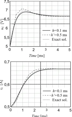
The time-response of capacitor voltage and inductor current will be computed for the time interval t∈[0,5ms]
.
These quantities are the state variables too. The corresponding discretized Euler companion diagram is shown in fig. 2.
h L 1 + n L U n C u 1 + n C u 1 + n C I E R1 R3 R2 C h J n L i 1 + n L i
Fig. 2. Discretized diagram.
According to the notations used in section II, we have:
= = = J E U I i u L C L
C X u
x ; ;
The computation way of the matrices E and F arises from the particular form of the expression (4):
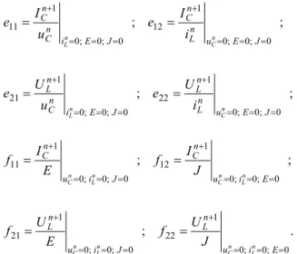
⋅ + ⋅ = + + J E f f f f i u e e e e U I n L n C n L n C 22 21 12 11 22 21 12 11 1 1 from where: ; ; ; ; 0 ; 0 ; 0 1 22 0 ; 0 ; 0 1 21 0 ; 0 ; 0 1 12 0 ; 0 ; 0 1 11 = = = + = = = + = = = + = = = + = = = = J E u n L n L J E i n C n L J E u n L n C J E i n C n C n C n L n C n L i U e u U e i I e u I e . ; ; ; 0 ; 0 ; 0 1 22 0 ; 0 ; 0 1 21 0 ; 0 ; 0 1 12 0 ; 0 ; 0 1 11 = = = + = = = + = = = + = = = + = = = = E i u n L J i u n L E i u n C J i u n C n L n C n L n C n L n C n L n C J U f E U f J I f E I f
Using the diagram of fig. 2, the elements of the matrices E and F were computed, assuming a constant time step
ms 1 . 0 = h : = − − − = 7519 , 0 0752 , 0 8270 , 0 0827 , 0 , 7740 , 9 7519 , 0 7519 , 0 1729 , 0 F E
The matrices M and N given by eq. (6), (7) are:
, 9023 , 0 0075 , 0 7519 , 0 8271 , 0 10 10 1 0 0 10 100 1 10 1 . 0 1 0 0 1 3 6 3 − = = ⋅ ⋅ ⋅ ⋅ ⋅ + = − − − E M . 0075 , 0 0008 , 0 8270 , 0 0827 , 0 10 10 1 0 0 10 100 1 10 1 , 0 3 6 3 = ⋅ ⋅ ⋅ ⋅ ⋅ = − − − F N
Starting from the obvious initial condition
= = A V i u L C 5 . 0 5 0 0 0 x ,
the solutions were computed using (8) and represented in fig. 3 with solid line.
The calculus was repeated in the same manner for a longer time step, h/ =5h=0,5ms, the solution being shown in the same figure. Both computed solutions are referred to the exact solution represented with thin dashed line.
V. CONCLUSION
computation of nonlinear dynamic networks.
The versatility of the method has already allowed an extension, in connection to the modified nodal approach.
uC
[V]
5 6 7
1 2 3
Time [ms]
4
0 5
6,5
5,5 7,5
h=0.1 ms
h’=0.5 ms Exact sol.
iL
[
A
]
1 2 3
Time [ms]
4
0 5
0,5 0,6 0,7
h=0.1 ms
h’=0.5 ms Exact sol.
Fig. 3. Circuit response.
ACKNOWLEDGMENT
This work was supported in part by the Romanian Ministry of Education, Research and Innovation under Grant PCE 539/2008.
REFERENCES
[1] A. Henderson, Electrical networks, London: Edward Arnold, 1990, pp.319-325.
[2] D. Topan, Computerunterstutze Berechnung von Netzwerken mit zeitdiskretisierten linearisierten Modellen, Wiss. Zeitschr. T.H. Ilmenau, 1978, pp. 99-107.
[3] C. Gear, The Automatic Integration of Ordinary Differential Equations, ACM, vol. 14, no. 3, 1971, pp.314-322.
[4] D. Topan, L. Mandache, Chestiuni speciale de analiza circuitelor electrice, Craiova: Universitaria, 2007, pp. 115-143.
[5] D. Topan, Iterative Models of Nonlinear Circuits, Annals of the University of Craiova, Electrotechnics, nr. 19, 1995, pp. 44-48. [6] R.A. Rohrer, Circuit Theory: An Introduction to the State Variable
Approach, New York: Mc Graw-Hill, Chap. 3-4, 1970.
[7] L. O. Chua, P. M. Lin, Computer-Aided Analysis of Electronic Circuits – Algorithms and Computational Techniques, Englewood Cliffs, NJ: Prentice-Hall, Chap. 8-9, 1975.
[8] W.-K. Chen, Active Network Analysis, Singapore: World Scientific, 1991, pp. 465-470.
[9] A. Opal, Sampled Data Simulation of Linear and Nonlinear Circuits, IEEE Trans. on Computer-Aided Design of Integrated Circuits Syst., vol. 15, no. 3, March 1996, pp. 295-307.