Data based on a Univariate Score
Glen A. Satten1*, Andrew S. Allen2, Morna Ikeda3, Jennifer G. Mulle3,4, Stephen T. Warren4
1Division of Reproductive Health, Centers for Disease Control and Prevention, Atlanta, Georgia, United States of America,2Department of Biostatistics and Bioinformatics and Duke Clinical Research Institute, Duke University, Durham, North Carolina, United States of America,3Department of Human Genetics, Emory University, Atlanta, Georgia, United States of America,4Department of Epidemiology, Emory University, Atlanta, Georgia, United States of America
Abstract
Motivation: The discovery that copy number variants (CNVs) are widespread in the human genome has motivated development of numerous algorithms that attempt to detect CNVs from intensity data. However, all approaches are plagued by high false discovery rates. Further, because CNVs are characterized by two dimensions (length and intensity) it is unclear how to order called CNVs to prioritize experimental validation.
Results:We developed a univariate score that correlates with the likelihood that a CNV is true. This score can be used to order CNV calls in such a way that calls having larger scores are more likely to overlap a true CNV. We developed cnv.beast, a computationally efficient algorithm for calling CNVs that uses robust backward elimination regression to keep CNV calls with scores that exceed a user-defined threshold. Using an independent dataset that was measured using a different platform, we validated our score and showed that our approach performed better than six other currently-available methods.
Availability:cnv.beast is available at http://www.duke.edu/,asallen/Software.html.
Citation:Satten GA, Allen AS, Ikeda M, Mulle JG, Warren ST (2014) Robust Regression Analysis of Copy Number Variation Data based on a Univariate Score. PLoS ONE 9(2): e86272. doi:10.1371/journal.pone.0086272
Editor:Marie-Pierre Dube´, Universite de Montreal, Canada
ReceivedApril 12, 2013;AcceptedDecember 12, 2013;PublishedFebruary 7, 2014
This is an open-access article, free of all copyright, and may be freely reproduced, distributed, transmitted, modified, built upon, or otherwise used by anyone for any lawful purpose. The work is made available under the Creative Commons CC0 public domain dedication.
Funding:MI, JGM, and STW are supported, in part, by NIH grants MH080129 and MH083722 and by the Simons Foundation (to STW). JGM was supported by a NIH fellowship award (MH080583). ASA is supported by NIH grants HL077663 and MH084680. The funders had no role in the study design, data collection and analysis, decision to publish, or preparation of the manuscript.
Competing Interests:The authors have declared that no competing interests exist.
* E-mail: [email protected]
Introduction
In any procedure for calling CNVs, there will be false positive calls made. While it may seem clear that CNV calls that are longer and/or feature a larger change in log intensity ratio (LIR) are more likely to be validated, it is not clear how to combine length and LIR information into a single measure that can be used to rank CNV calls. Optimally, such a measure would correlate with the chance that a CNV would be experimentally validated. All current methods of calling CNVs are in some way based on statistical information,e.g.based on a p-value for a hypothesis test or a posterior probability from a Bayesian model, to determine whether a series of adjacent probes should be considered a CNV. It is not cleara priorithat statistical information is the best predictor of whether a CNV will validate, and assessing this proposition is the first goal of our paper.
To develop a univariate measure that predicts experimental validation, we introduce a family of scores of the formmma, where
m is a measure of CNV intensity and mis a measure of CNV length. We choose the exponentaso that the resulting score is the best predictor of experimental validation. We made this choice using data on log intensity ratios (LIRs) measured using a Nimblegen array comparative genome hybridization (aCGH) platform, with calls made by the Nimblescan software. For a
subset of 111 putative CNVs, we used gel electrophoresis of PCR products to determine which calls corresponded to true CNVs.
Because our score is chosen to correlate with the chance a CNV is validated, we wanted to make calls based on this score; in particular, we wanted a fast, easy-to-use algorithm that would call CNVs based on their score, keeping those that exceed a user-specified minimum score. To this end, we developed cnv.beast (backward elimination algorithm with score-based threshold), a novel regression-based computationally-efficient algorithm for calling CNVs.
Additional methods for calling CNVs include wavelet-based methods [2], smoothing approaches [3], and hierarchical cluster-ing [4]. Additional approaches are described by [5] and [6].
Three regression-based algorithms for finding CNVs are currently available: GLAD [7], a 1-dimensional version of a smoothing-based non-parametric regression approach developed for analyzing 2-dimensional images, and two approaches based on the Lasso [8], [9]. In our experience, the parameters for GLAD are hard to tune and do not have simple interpretations; further, GLAD is computationally intensive. The Lasso-based approach also has several drawbacks. First, the choice of smoothing parameters can be ad-hoc [8] or complex [9], leading to limitations on the number of probes that can be fit [5]. Further, it is not clear that the global optimization criterion used by the lasso corresponds to a good choice of CNVs. For example, small shifts in intensity over a large number of probes may be selected by the lasso but are unlikely to correspond to CNVs. Thus we seek an algorithm tailored to the problem of CNV detection.
The remainder of the paper is organized as follows. We first analyze a set of experimentally-validated calls made using Nimblegen data on the X-chromosome to determine a score function that correlates with the chance that a called CNV overlaps with a true CNV. We then develop cnv.beast, a novel backward-elimination regression algorithm that keeps CNVs having scores that exceed a user-defined threshold. Finally, we validate our approach by using data on deletions in eight Hapmap samples that have been experimentally determined [10]. Ely [5] compared the ability of six previously-published methods to use data from the Illumina 1M chip to detect the CNVs found by Kidd et al. [10]. By analyzing these data with our algorithm, we can assess the performance of our approach relative to existing algorithms for calling CNVs.
Ordering CNVs by a Score that Predicts Validation We assume that the observed data comprise the log-intensity ratio (LIR) values at a series of probes having known position in the genome, either from an aCGH experiment or from quantitative intensity data from a genotyping platform (i.e., Illumina or Affymetrix), compared to a reference population. Suppose that from these data, a set of putative CNVs have been proposed. For each called CNV, letmdenote a measure of the ‘length’ of the CNV (here we use the number of probes that comprise the CNV) and letmdenote a measure of the intensity or ‘height’ of a CNV (here we use the absolute value of the median LIR across probes that comprise the CNV). We seek a univariate score of the formmmato assign each putative CNV. The choice
a~1=2 corresponds to statistical information [6], in that a statistical hypothesis test (e.g., at-test) of whether the intensities of the probes comprising the CNV are significantly different from zero would be proportional tomm1=2. We wish to chooseaso that
high-scoring CNVs have a greater chance of being validated (true). To choose the value ofafor the score, we used data on copy number variation on the X chromosome for 41 human males whose DNA is available through the Autism Genetics Resource Exchange (AGRE) [11]. The copy number status of each individual’s X chromosome was queried using three non-overlapping but contiguous Nimblegen comparative genome hybridization (CGH) sub-arrays. Each sub-array had approxi-mately 700,000 probes, so that a LIR was measured at 2,020,823 probes on the X chromosome for each individual. The X chromosome sequence was repeat masked and the PAR1 and PAR2 regions were removed prior to probe selection. This resulted in an average intermarker distance of 50 base pairs or 20 probes/kilobase.
Copy number variants were called using the NimbleScan (NS) software package version 2.4, an implementation of circular binary segmentation analysis, distributed by Nimblegen. Each sub-array was analyzed separately. Data from non-unique probes as well as data from approximately 5% of poorly-behaving probes having unusually large variance was discarded. Spatial correction and normalization were performed using NS, then segment boundaries were determined using the default parameters (no minimum difference in LIR that segments must exhibit before they are identified as separate segments; two or more adjacent probes required to call a change in LIR; maximum stringency for selecting initial segment boundaries).
The NS package gives a list of segment boundaries; because change in LIR across boundaries may be negligible, segment boundaries do not necessarily correspond to CNVs. We selected as CNVs those segments for which the absolute value of the mean LIR was greater than the absolute value of the sum of the mean LIR for the sub-array LIR plus one standard deviation. To identify a parsimonious set of segments for validation, CNVs were merged if their endpoints were within 3kB and if their mean LIRs had the same sign. The LIR of the merged CNV was taken to be the
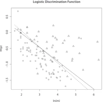
Figure 1. Logistic discrimination functions for Nimblegen X-chromosome data corresponding to optimal score (a= 0.44, solid line) and statistical information score (a= 0.5, dashed line).Triangles correspond to true positives, ellipses to false positives. doi:10.1371/journal.pone.0086272.g001
Table 1.Choice of Parameters in Cutoff Function.
Parameter Default Value
mmin 6
mmax 30
mmin 0.25
a 0.5
weighted average of the unmerged LIRs, weighted by the number of probes. Finally, to increase reliability, CNVs were only called if the probe density was greater than 9 probes/kB (i.e., slightly less than half of the average probe density for these data, 20 probes/ kB).
Using Nimblescan as described above, we obtained 414 putative CNVs. Experimental determination of validation status using PCR amplification followed by gel electrophoresis was successfully completed for 111 putative CNVs called among 41 persons. For generalizability to multiple platforms, we quantile normalized the LIR data before further analysis. Based on examination of both the X-chromosome data described above and data from Affyme-trix arrays (data not shown), we chose to quantile normalize to at
distribution with 5 degrees of freedom, scaled so that the median absolute deviation (MAD) was 0.2. For each called CNV we counted the number of probesmand took the intensitymto be the absolute value of the median LIR for the quantile-normalized data.
We fit a logistic regression model with validation status (V= 1 if validated,V= 0 if not) as the outcome, using the log of the absolute intensity ln(m) and the log of the number of probes ln(m) as predictor variables,i.e.
lnPr½V~1jm,m
Pr½V~0jm,m~a1za2ln (m)za3ln (m) ð1Þ
CNVs found in the same individual as well as overlapping CNVs found in multiple individuals were treated as independent when fitting this model. The region ofmandmvalues whereV= 0 is more likely and the region ofmandmvalues whereV= 1 is more likely is separated by the decision boundary where
Pr½V~1jm,m~Pr½V~0jm,m,which corresponds to the line
ln (m)~{a1 a3
{a2 a3
ln (m) ð2Þ
Note that for any scoring function of the form S~mma, contours of constant score are also straight lines of the form (2)
with a1 a3
~{ln (S) and a2 a3
~a. Scoring based on statistical
information thus corresponds toa2 a3
~1
2.
By fitting the logistic model, we found^aa2 ^ a a3
~0:44and that a 95% confidence interval for^aa2
^ a a3
obtained using the delta method (on the
log scale) was (0.32, 0.59). Figure 1 shows a plot of validation status by ln(m) and ln(m), with the logistic regression discrimination function (2). Visual examination of Figure 1 suggests that a scoring function of the formmma is valid, as the proportion of validated CNVs increases perpendicular to lines of constant score. Note that
the choicea~1
2lies in the confidence interval foraand is thus
consistent with these data. In Figure 1 we also plot the discrimination function obtained by fitting model (1) subject to
the restriction^aa2 ^ a a3
~1
2. Visual examination of Figure 1 shows that
the restricted model predicts experimental validation almost as well as the unrestricted model. Thus, statistical information as
measured bymm1=2 correlates with experimental validation, and for all subsequent analyses in this paper, we used the choicea~1
2.
A Regression Approach to CNV Calling using a Backward Elimination Algorithm with a Score-based Threshold
We describe cnv.beast, a novel backward elimination algorithm for regression analysis of CNV data that is based on the availability of a univariate score function for ordering CNVs. The algorithm is based on a regression model in which LIR data from an individual is regressed on a series of step functions having jumps at each probe. We treat each step function (jump) as a CNV (with length given by the distance to the nearest jump and height given by the change in predicted magnitude) so that a score for each term can be calculated. Then, the algorithm implements backward elimi-nation until each term in the regression model has a score higher than a user-specified cutoffS*, while also eliminating CNVs that contain fewer thanmminprobes or have intensity less thanmmin. Any
univariate scoring function can be used; here we use mma with
a~1
2.
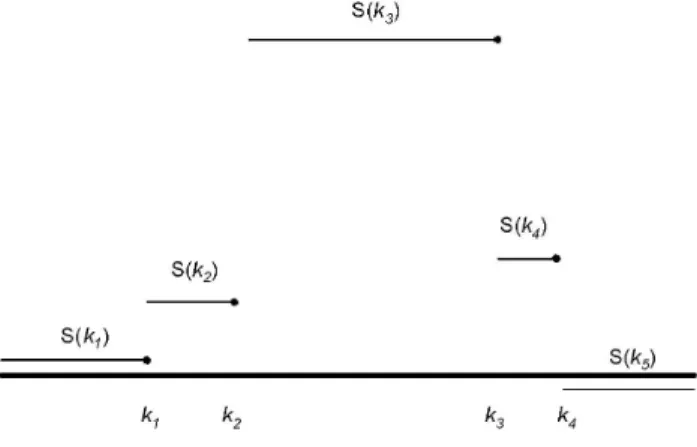
Figure 2. Illustration of situation where removed jump does not have smallest value ofd.As illustrated, we would remove the probe atk2rather than the probe atk1, and then the probe atk4rather than the probe at k3 even though d1vd2 and d3vd4 The solid horizontal line corresponds to a log-intensity ratio of 0.
doi:10.1371/journal.pone.0086272.g002
Figure 3. Illustration of cleanup step.As the backward elimination step has terminated, each jump is larger than the appropriate cutoff. At the start of the cleanup step,S(k1) and S(k3) would be set to zero, decreasingjb(k3)j~jS(k4){S(k3)jand hence making it a candidate for removal if it becomes smaller than the appropriate cutoff.
We use backward elimination to avoid masking. Masking occurs in forward selection algorithms when a term that would correspond to one boundary of a CNV is not entered into the model because the term that corresponds to that CNVs other boundary is not yet in the model. For example, a CNV comprised of probes 80–120 would be described by two terms in equation (3):
b(k79)I½iwk79and b(k120)I½iwk120. A forward selection
algo-rithm that adds these terms one at a time may find that neither term should be added by itself. By using backward elimination, and by starting with a possible term at each probe, we hope to avoid masking.
We advocate quantile normalization of the log intensity ratios even if the numerator and denominator have already been normalized, so that the same cutoffs can be used for all datasets. As described previously, we normalized to a student t distribution with 5 degrees of freedom, scaled so that the median absolute deviation was 0.2. We made this choice so that our cutoffs for quantile normalized data could also be reasonably applied to untransformed data if necessary.
Regression Analysis of CNV Data
Letyi,i~1, ,N denote the log intensity ratio for data onN
probes from a single chromosome or chromosomal subregion for a single individual. The goal of our analysis is to fit step functions to theyis to determine the locations of the jumps (places where the copy number may change) and the magnitude of these changes. We assume that the (normalized or centered)yican be described using the model
yi~ X J{1
j~1
b(kj)I½iwkjzei ð3Þ
where kj is the location (probe number) of thejth of J change points,b(kj) is the change in log intensity ratio between probekj
and kj+1 andI½iwk~1ifi.kand 0 otherwise. Our goal is to select the change points kj and the values b(kj). We denote the resulting step function fit to the datayiby
S(t)~X
J{1
j~1
b(kj)I½twkj, k1vtvkJ
While it is possible to determine fit by using least squares,i.e.by minimizing
yi~ X J{1
j~1
b(kj)I½iwkj !2
, ð4Þ
we instead propose a robust regression approach that minimizes
yi~ X J{1
j~1
b(kj)I½iwkj
, ð5Þ
which is robust to isolated large values that are present in CNV data even after quantile normalization.
WhenJ~Nand consequentlykj~j, the model is saturated and
has(N{1)jumps (i.e., takes a different value between each probe). This model is clearly over-fit. When using least squares, one approach to thinning the set of jumps is to use the Lasso, which corresponds to minimizing the saturated model (4) subject to the
constraint that JP {1
j~1 b(j)
j jƒl for some appropriately chosen
smoothing parameter l [2], [9]. Here we adopt a different approach which is specifically tailored to the CNV problem, is computationally efficient when using (5), and features a novel backward-elimination algorithm that allows control of the intensity, length and score of CNVs that are detected.
Our backward elimination algorithm begins with the saturated model(J~N)havingN{1terms, and removes one term from (3) at each step. Thus, at the beginning of therth step, there areN{r terms in the model; we denote the probes that are in the model at the start of the rth step by k(1r),k2(r), ,k(Nr){r. At each step, we
remove a single jump,i.e.we remove a single valuekj(r) from the set of jumps.
Backward elimination is facilitated by the following observa-tions. First, the values ofb(j) that minimize either (4) or (5) for the saturated model are
^ b
b(j)~yjz1{yj,
so that the saturated model can be easily fit. Second, at therth step of backward elimination, the least-squares estimator ofbb^(k(jr))is
^ b b(kj)~
1
kj(zr)1{k (r) j
! X k(r)
jz1
i~k(jr)z1
yi{
1
kj(r){k(r)
j{1
! X kj(r)
i~k(r) j{1z1
yi,
while the L1 estimator ofbb^(kj(r))is
^ b b(kj)
~median yi,kj(r)viƒk (r) jz1
n o
{median yi,k(j{r)1viƒk (r) j n oð6Þ
Importantly, note that removing a term from (3), say k(jr), only
affects the values of bb^ k(jr){1
and ^bb kj(r)z1
. As a result,
backward elimination can be carried out very efficiently; for each term removed it is only necessary to update the two adjacent coefficients.
Backward Elimination using a Score-Based Threshold Algorithm, and the Cutoff Function
We now describe how we choose which jumps to eliminate so that only CNVs having ‘large’ scores are retained. We define the ‘gap’ between the probek(jr)and the nearest probes remaining in
Table 2.CNV.BEAST calls and Validation Status.
Validation Detected by CNV.BEAST
Status: Yes No
True 38 6
False 50 17
the model (i.e., probes for which bkj(r)=0) to be g(jr)~mink(jr){kj{(r)1,k(jzr)1{k(jr) with the convention that kN(r){rz1~N and k
(r)
0 ~1. Thus, the gj is simply the distance to
the nearest jump. We wish to eliminate terms for which the change in intensity is ‘small,’ considering the size of the gap. Noting that
b(kj) is the magnitude of the change in intensity at probe kj, we therefore wish to keep the jump atkjonly if the score b(kj)
gaj is
‘large.’ This suggests that we keep terms for which
b(kj)
§D
ga
j
,
for some valueD. However, we also wish to ensure that all CNVs that are kept are comprised of at leastmminprobes. To avoid jumps
of very small magnitude that involve many probes, we also require that CNVs comprised of more thanmmaxprobes also have intensity
larger thanmmin. To accomplish all of these goals, we replace the
cutoffD=ga
j by the cutoff functionC(g), defined by
C(g)~
M, gvmmin
mminma
max
ga , mminƒgvmmax
mmin, mmaxƒg
8 > > <
> > :
whereMis some very large number (say, 1016) that is much larger than the absolute value of the largest log intensity ratio in the data. The ‘default’ values of the parameters mmin, mmaxand mmin were
selected based on our experience with our algorithm, and are given in Table 1. Users may vary these parameters in our software implementation, if they so desire.
Having chosen the form of the cutoff functionC(g), we take as the goal of our algorithm that, at termination, we should have
b(k(jr))
§C g
(r) j
ð7Þ
for all terms remaining in the model. To this end, we define Figure 4. Logistic discrimination functions for Illumina Hapmap data corresponding to optimal score (a= 0.59, solid line) and statistical information score (a= 0.5, dashed line).Triangles correspond to true positives, ellipses to false positives.
doi:10.1371/journal.pone.0086272.g004
Table 3.Comparison of Sensitivity and FDR.
Method #of calls Sensitivity1
#of calls
.6kbp FDR2
Circular Binary Segmentation
315 0.218 104 0.788
Hidden Markov Model
20,226 0.287 1,081 0.957
Segmentation/ Cluster
837 0.208 55 0.691
Wavelet-based Segmentation
13,665 0.198 187 0.840
Fused Lasso 655 0.248 130 0.808
Robust Smoothing
37 0.059 29 0.690
CNV.BEAST 195 0.299 167 0.826
1Sensitivity is the number of true deletions that overlap at least partially with a called deletion, divided by the number of true deletions.
2FDR is the number of called deletions that do not overlap even partially with a true deletion, divided by the number of called deletions.
d(jr)~b(k(jr))
{C g
(r) j
;
note that d(jr)v0 if the jump at k(jr) violates (7) and d (r) j §0
otherwise. Thus, in general, we choose to remove the jump atk(jr) that corresponds to the smallest (i.e.,the most negative) value of
dj(r). When kj(r) is removed, b kj(r){1
, b kj(r)z1
, g(jr){1, g (r) jz1, d(jr){1, and d
(r)
jz1 are updated, concluding the rth step of the
algorithm. The algorithm is terminated at the first stepr*for which
d(jr)§0 for 1ƒjvr{1, at which point all remaining jumps satisfy (7).
Our backward elimination algorithm can be efficiently executed with a single pass through a sorted list of the values ofd(jr). After each step, there are only three values ofd(jr)that are out of order;
d(jr){1,d (r) j and d
(r)
jz1so that it is easy to update the list of sorted
values ofd(jr)required for subsequent steps of the algorithm.
Alternative Selection Criterion for Adjacent Jumps in the Same Direction
As described above, we choose to remove the jump atk(jr) that
corresponds to the smallest (most negative) value ofd(jr). In some situations, as illustrated in Figure 2, this is unwise. Note that for this situation, b(k2):S(k3){S(k2)w b(k1):S(k2){S(k1)w
while g1~g2 (because the probes at k1 and k2 are each their
closest neighbors) so that d1vd2, suggesting that we remove k2
beforek1. Similarly, we may be tempted to removek3beforek4. However, this may under-estimate the true length of the CNV. Worse, if the (remaining) jumps atk2andk3satisfyk3{k2ƒmmin,
they will be removed and a CNV will not be called. Thus, whenever two adjacent jumps occur in the same direction that take
S(k) further from zero, the first jump will be kept in preference to the second (even ifdfor the first jump is smaller than the second). Similarly, whenever two adjacent jumps occur in the same direction that result inS(k) being moved closer to zero, the second jump will be kept in preference to the first (even ifdfor the second
jump is smaller than the first). Formally, these conditions can be stated as follows. When considering whether to remove a probe at positionk(jr), we instead remove the probe at positionk(jzr)1if: (1)
bk(jr)b k(jrz)1
w0, (2)k(jr){kj({r)1wmminandk(jzr)1{k (r) j ƒmmin,
and (3) S k(jrz)2
w S k
(r) j
Similarly, when considering whether to remove a probe at positionk(jr), we instead remove
the probe at position k(j{r)1 if: (1) b k (r) j{1
bk(jr)w0, (2) k(jr){k
(r)
j{1ƒmmin and kj(zr)1{k (r)
j wmmin, and (3) S kj(zr)1
w
S kj({r)1
.
Overlapping Blocks for Large Probesets
Although our algorithm is computationally efficient, calculating medians for large numbers of probes between CNVs slows the algorithm as the number of probesNincreases. To handle datasets with large numbers (,200,000) of probes, we have developed a
variant of our algorithm that breaks the calculation into overlapping blocks ofM probes. The mth such block comprises
data yi on probes
(m{1)M
2 z1ƒiƒ
(mz1)M
2 for 1ƒmƒ 2N
m{1; a final block comprising data yi on probes N{Mz1ƒiƒN is also used. The algorithm described above is then implemented on each block. Then, the algorithm is restarted using datayion all probes, but only allowing terms into model (3) that were retained in at least one of the block analyses. WhenMis sufficiently large (50,000 probes) we have observed negligible difference in the output of the block and standard versions of our algorithm. We analyzed data on chromosome 2 from 104 individuals, each data set having 148,812 probes, and found no differences in output when using 50,000 (corresponding to 5 blocks) and the analysis done in a single block. The block algorithm can substantially reduce the run time for largeN. For example, an analysis of 700,000+ probes that took 9Kminutes, when run as a single block, completed in 1Kminutes when run using 15 blocks of 50,000 probes, with identical results. Timings are for a core duo laptop with a 2.53 GHz clock speed and 3 GB RAM.
The Cleanup Step
At the termination of the algorithm just described (either with or without the use of blocks), the log-intensity ratios predicted by (3) form a step function in which each jump is ‘large enough’ compared with the gap between adjacent retained probes to satisfy our model selection criterion (7). However, because we have not required that the predicted log-intensity ratio return to zero between adjacent CNVs, it can occur that the predicted intensity between probes is actually less thanmmin(see Figure 3). Thus, once
the algorithm has terminated, we implement a ‘cleanup step’ in which we re-start the backward elimination (treating the entire data as a single block) with the requirement that all predicted values be either zero or greater than mmin. This corresponds to
replacing (6) with
^ b
b(kj)~h median yi,k(jr)viƒk (r) jz1
n o
;mmin
{h median yi,k(r)
j{1viƒk (r) j
n o
;mmin
whereh(x;mmin)~xifj jx§mminand 0 otherwise.
Finally, even after the cleanup step, some regions may have several jumps before returning to zero. Typically, this occurs for long CNVs. When the predicted LIR has the same sign over the entire region, we use the average intensity over the region, weighted by the number of probes. In those rare cases where a sign change occurs, we consider the probe at which the sign changes to be a boundary between two (adjacent) CNVs. Thus, if a region has first positive and then negative LIR values, we could consider that two CNVs are adjacent; if this occurs, we separately average the predicted intensities over any jumps occurring in regions where the LIR was positive and negative. Scores are then calculated using the length of the region and the averaged intensity.
Validation using Experimentally Verified Samples We first applied our algorithm to the Nimblegen data that we used previously to determine the score exponenta. Here our goal is to compare the quality of the calls made by Nimblescan to those made by cnv.beast. Of the 111 Nimblescan calls that we have determined validation status experimentally, 44 were found to be true. Using the parameter values in Table 1, cnv.beast detected 88 of the 111 calls; however, of the 23 calls missed by cnv.beast, 17 (74%) failed to experimentally validate (see Table 2). Overall, cnv.beast made 638 calls compared with 414 calls made using our filtering of the calls made by Nimblescan.
To assess the performance of our approach in an independent dataset, we analyzed Illumina 1M data from eight Hapmap participants. Deletions among these individuals were determined experimentally by Kidd et al. [10] using fosmid-ESP with additional confirmation by a second method. Deletions in these data were also called by Ely [5] using six CNV-calling programs, allowing us to compare the performance of cnv.beast with previously-existing methods. The methods chosen (and the names of the R packages used) were circular binary segmentation analysis [12] (DNAcopy), hidden Markov partitioning [13] (aCGH), segmentation-clustering [14] (segclust), wavelet segmentation [2] (waveslim), fused lasso segmentation [9] (FLasso), and robust smooth segmentation [3] (smoothseg). The last three methods also utilized the R package ‘cluster’.
We first validated that our choice of CNV score was predictive of validation in these data by fitting the logistic regression model (1) to quantile-normalized data. We found good agreement between the exponent we obtained using Nimblegen X-chromosome data and the Illumina data; the estimated exponent was 0.59 with
95% confidence interval (0.34, 1.04). In Figure 4 we compare
the best-fitting logistic model to the case a~1
2. Comparing
Figure 4 with Figure 1, we note the higher proportion of false positive calls due to the exhaustive enumeration of deletions in these data compared with the more selective approach taken in the Nimblegen data.
Cnv.beast performed well when compared to the six methods considered by Ely (see Table 3). Details of the implementation of these six methods in these data can be found in Ely (2009). We note first that our algorithm processed data from all eight individuals in 6K minutes on a core duo laptop with a 2.53 GHz clock speed and 3 GB RAM. Note that cnv.beast had the second smallest number of calls (195) but the highest proportion of true deletions that were at least partially covered by a called region (29.9%). To compare with Ely, we calculated the false discovery rate (FDR) only for calls that exceeded 6000 base pairs in length. Of the 167 calls we made that exceeded this threshold, 138 did not overlap with a true deletion, for a false discovery rate of 82.6%. The only methods with notably lower FDR made fewer true discoveries (9 for SmoothSeg and 17 for SegClust) than the 29 we made.
Although the FDR of cnv.beast was 82.6% overall, it is possible to achieve lower FDRs by further filtering the list of called CNVs to those having score greater than some specified value. For example, the FDR for our method among calls made by cnv.beast using the default parameters in Table 1, that further have score greater than 2.5, is 69.2% while the FDR for calls having score greater than 5 is 50%. Considering only calls with score greater than 2.5 where the FDR of our method is comparable to SegClust (17) and SmoothSeg, our method finds 20 true deletions, more than found by either SegClust or SmoothSeg (9). These results suggest that overall, our method outperforms the six competing methods compared by Ely [5]. A plot of the empirical FDR is given in Figure 5. This plot suggests that the score is very useful in prioritizing which calls to experimentally validate.
Discussion
CNVs are characterized by both height (intensity) and length (number of probes), making it difficult to predict which calls are valid. Using X-chromosome high-density Nimblegen array CHG data, we propose a univariate score that incorporates both intensity data and the number of probes in a call, and that predicts the probability a CNV is valid. We then showed that the same score is a valid predictor of experimental validation in Illumina gene chip data.
Based on the concept of a univariate score, we then developed cnv.beast, a novel backward elimination regression algorithm that keeps terms corresponding to CNVs that exceed a user-defined threshold. Using data from eight Hapmap participants, we showed that cnv.beast had superior performance when compared to the six other methods considered by Ely [5]. Cnv.beast has been successfully used to find CNVs that are risk factors for schizophrenia and autism [15–17].
As a univariate quantity, the score can facilitate Monte-Carlo significance testing. Specifically, if we can generate replicate datasets that are known to have no signal, then for each replicate dataset, we can record the largest score found among all CNVs detected. This distribution can then be used to assign ap-value to the CNVs observed in the original data. Hypothesis testing of this type is difficult without a univariate measure to order CNVs. Further, cnv.beast, which is fast even for datasets with many probes, is ideal for this kind of Monte-Carlo analysis. This approach has been implemented by Satten et al. (2012) [18].
Many algorithms for calling CNVs were initially developed for data from cancer cell lines, where copy number changes are often long and hence may be easier to detect. As Table 3 illustrates, the data quality of current CNV platforms is poor when applied to DNA from normal cells, regardless of the algorithm used for calling variants. In order to be useful for association studies (the goal of many studies that use CNVs) it is currently necessary to validate CNV calls using a second technology. Because experi-mental validation is laborous, slow and expensive, a predictor of validation status such as the score we propose, could be useful in
prioritizing which CNV calls to validate, regardless of what algorithm is used to make the calls.
Software Availability
A fortran program to unleash the power of the beast, as well as an R shell to run it and a pdf file with usage notes, is available at http://www.duke.edu/,asallen/Software.html.
Acknowledgments
We thank Li Hsu and Ben Ely for graciously giving us access to the HapMap data and early access to Ben Ely’s Master’s thesis.
Disclaimer: The findings and conclusions in this report are those of the authors and do not necessarily represent the official position of the Centers for Disease Control and Prevention.
Author Contributions
Conceived and designed the experiments: GS JM SW. Performed the experiments: JM MI. Analyzed the data: GS AA. Wrote the paper: GS AA JM.
References
1. Wang K, Li M, Hadley D, Liu R, Glessner J, et al. (2007) An integrated hidden Markov model designed for high-resolution copy number variation detection in whole-genome SNP genotyping data. Genome Research 17: 1665–1674. 2. Hsu L, Self S, Grove D, Randolph T, Wang K, et al. (2005) Denoising
array-based comparative genomic hybridization data using wavelets. Biostatistics 9: 211–226.
3. Huang J, Gusnanto A, O’Sullivan K, Staaf J, Borg A, et al. (2007) Robust smooth segmentation approach for array CGH data analysis. Bioinformatics 23: 2463–2469.
4. Xing B, Greenwood CMT, Bull SB (2007) A hierarchical clustering method for estimating copy number variation. Biostatistics 8: 632–653.
5. Ely B (2009) A comparison of methods for detecting copy number variants from single nucleotide polymporphism intensity data. Masters Thesis, Department of Biostatistics, University of Washington, Seattle WA.
6. Jeng XJ, Cai TT, Li H (2010) Optimal sparse segment identification with application in copy number variation analysis. Journal of the American Statistical Assocociation 105: 1156–1166.
7. Hupe P, Stransky N, Thiery J, Radvanyi F, Barillot E (2004) Analysis of array CGH data. Bioinformatics 20: 3413–3422.
8. Huang T, Wu B, Lizardi P, Zhao H (2005) Detection of DNA copy number alterations using penalized least squares regression. Bioinformatics 21: 3811– 3817.
9. Tibshirani R, Wang P (2008) Spatial smoothing and hot spot detection for CGH data using the fused lasso. Biostatistics 9: 18–29.
10. Kidd JM, Cooper GM, Donahue WF, Hayden HS, Sampas N, et al. (2008) Mapping and sequencing of structural variation from eight human genomes. Nature 453: 56–64.
11. Geschwind DH, Sowinski J, Lord C, Iversen P, Shestack J, et al (2001) The Autism Genetic Resource Exchange: a resource for the study of autism and related neuropsychiatric conditions. American Journal of Human Genetetics 69: 463–6.
12. Olshen A, Venkatraman E, Lucito R, Wigler M (2004) Circular binary segmentation for the analysis of array-based DNA copy number data. Biostatistics 5: 557–572.
13. Fridlyand J, Snijders A, Pinkel D, Albertson D, Jain A (2004) Hidden Markov models approach to the analysis of array CGH data. Journal of Multivariate Analysis 90: 132–153.
14. Picard F, Robin S, Lebarbier E, Daudin J (2007) A Segmentation/Clustering Model for the Analysis of Array CGH Data. Biometrics 63: 758–766. 15. Mulle JG, Dodd AF, McGrath JA, Wolyniec PS, Mitchell AA, et al. (2010)
Microdeletions in 3q29 Confer High Risk of Schizophrenia. American Journal of Human Genetics 87: 229–236.
16. Moreno-De-Luca D, SGENE Consortium, Mulle JG, Simons Simplex Collection Genetics Consortium, Kaminsky EB, et al. (2010) Deletion 17q12 is a Recurrent Copy Number Variant that Confers High Risk of Autism and Schizophrenia. American Journal of Human Genetics 87: 618–30. Erratum in: American Journal of Human Genetics 88: 121.
17. Mulle JG, Pulver AE, McGrath JA, Wolyniec PS Dodd AF, et al. (2013) Reciprocal Duplication of the Williams-Beuren Syndrome Deletion on Chromosome 7q11.23 is Associated with Schizophrenia. Biological Psychiatry in press.