Altitudinal Gradient in Gongga Mountain, China
Shou-Qin Sun*, Yan-Hong Wu, Gen-Xu Wang, Jun Zhou, Dong Yu, Hai-Jian Bing, Ji Luo
Key Laboratory of Mountain Surface Processes and Ecological Regulation, Institute of Mountain Hazards and Environment, Chinese Academy of Sciences, Chengdu, China
Abstract
An investigation of terrestrial bryophyte species diversity and community structure along an altitudinal gradient from 2,001 to 4,221 m a.s.l. in Gongga Mountain in Sichuan, China was carried out in June 2010. Factors which might affect bryophyte species composition and diversity, including climate, elevation, slope, depth of litter, vegetation type, soil pH and soil Eh, were examined to understand the altitudinal feature of bryophyte distribution. A total of 14 representative elevations were chosen along an altitudinal gradient, with study sites at each elevation chosen according to habitat type (forests, grasslands) and accessibility. At each elevation, three 100 m62 m transects that are 50 m apart were set along the contour line, and three 50 cm650 cm quadrats were set along each transect at an interval of 30 m. Species diversity, cover, biomass, and thickness of terrestrial bryophytes were examined. A total of 165 species, including 42 liverworts and 123 mosses, are recorded in Gongga mountain. Ground bryophyte species richness does not show any clear elevation trend. The terrestrial bryophyte cover increases with elevation. The terrestrial bryophyte biomass and thickness display a clear humped relationship with the elevation, with the maximum around 3,758 m. At this altitude, biomass is 700.3 g m22 and the maximum thickness is 8 cm. Bryophyte distribution is primarily associated with the depth of litter, the air temperature and the precipitation. Further studies are necessary to include other epiphytes types and vascular vegetation in a larger altitudinal range.
Citation:Sun S-Q, Wu Y-H, Wang G-X, Zhou J, Yu D, et al. (2013) Bryophyte Species Richness and Composition along an Altitudinal Gradient in Gongga Mountain, China. PLoS ONE 8(3): e58131. doi:10.1371/journal.pone.0058131
Editor:Ben Bond-Lamberty, DOE Pacific Northwest National Laboratory, United States of America
ReceivedJuly 12, 2012;AcceptedFebruary 4, 2013;PublishedMarch 5, 2013
Copyright:ß2013 Sun et al. This is an open-access article distributed under the terms of the Creative Commons Attribution License, which permits unrestricted use, distribution, and reproduction in any medium, provided the original author and source are credited.
Funding:The present work was supported by the ‘‘National Natural Science Foundation of China’’ (Grant No. 41273096, 30900201) and the ‘‘Knowledge Innovation Project of the Chinese Academy of Sciences’’ (Grant No. KZCX2-EW-QN310, KZCX2-YW-BR-20). The funders had no role in study design, data collection and analysis, decision to publish, or preparation of the manuscript.
Competing Interests:The authors have declared that no competing interests exist. * E-mail: [email protected]
Introduction
Bryophytes are an important component of ecosystem bio-diversity and make up a significant part of species richness [1–3] and plant biomass in forests in some cases [4,5]. They also play a prominent role in ecosystem functions, such as soil development [6,7], nutrient biogeochemical cycling [4,8], water retention [9], plant colonization [10], seed germination, seedling growth, and forest renovation [5,8,11]. However, bryophytes are still rarely considered in biodiversity surveys when compared with their vasular counterparts [12]. The reasons include difficulties in identification, fewer specialists, less literatures on bryophyte taxonomy in tropical areas, and the high-costs (both time and money) for searching and identifying bryophytes. Bryophytes have wider distribution and longer altitudinal gradient than vascular plants, and thus strong generalizations on observable changes in diversity along latitudinal and altitudinal gradients can be made according to bryophyte distribution if any patterns do exist [13]. They therefore have been deemed as ideal candidates for altitudinal studies in recent years [13]. With growing interest in climate change, using bryophytes as indicator species for climate change has also attracted more attention due to their sensitivity to environmental change [14]. Research on bryophyte diversity, richness and distribution is therefore increasing [12,15].
Several altitudinal patterns of bryophyte richness and distribu-tion have been reported, such as decreasing [16] or increasing
[12,17–19] with elevation increasing, a hump-shaped distribution [15] and no obvious trends at all [13]. Although there still is no explanation for these differences, it is now widely accepted that peak diversity coincides with optimum environmental conditions [12]. However, various factors such as forest properties include stand structure [20], canopy opening [21,22], forest management [23], and climate [24,25] can cause variation in species richness, growth rate, and community structure of bryophytes.
influences the diversity and distribution of ground and field-layer species.
Views about the factors mainly influencing bryophyte growth and distribution are still debated. The ecological mechanisms of bryophyte richness and distribution pattern along altitudinal gradients still need to be further investigated. In addition, the biomass, thickness and cover of bryophytes are key indices reflecting bryophyte growth status. Such data are useful for modeling whole ecosystem response to climate change, modeling ecosystem carbon and nutrient cycling, and improving our understanding of the ecological roles of bryophytes in forest ecosystem. However, most of the previous research did not consider the biomass, thickness and cover of bryophytes.
The objectives of the present study were (1) to describe the distribution pattern of terrestrial bryophytes along an altitudinal gradient in Gongga Mountain, Sichuan, China, and (2) to find out the major factors which influence bryophyte diversity and distribution. This investigation will be helpful in identifying strategies and opportunities for the conservation of bryophyte species, and would also be the basis of climate change research in this area. We hypothesized that climate is the main factor that influences bryophyte distribution.
Methods
Study Area
The study was conducted in Gongga Mountain (29u209- 30u209
N, 101u309- 102u159E), which is located in Sichuan, southwestern China, at the eastern edge of the Tibetan Plateau. The peak of Gongga Mountain is 7556 m a.s.l., the summit in the Hengduan Mountain Range. Within a horizontal distance of 28 km the relative height drops 6,400 m to the eastern bottom of Gongga Mountain. On the eastern slope of Gongga Mountain, the annual precipitation varies between 1,068 and 3,210 mm (increases with the elevation below 3,650 m a.s.l., but decreases with the elevation above 3,650 m a.s.l.), the mean annual temperature is between
22.6 and 14.5uC depending on the altitude. The mountain has an intact vertical zonality from subtropical vegetation to alpine cold vegetation [31]. The vegetation in the study area varies from evergreen broad-leaved forest (1,600–2,200 m a.s.l.), mixed evergreen and deciduous broad-leaved forest (2,200–2,400 m a.s.l.), mixed broadleaf-conifer forest (2,400–2,800 m a.s.l.), dark coniferous forest (2,800–3,600 m a.s.l.), alpine shrubland (3,600– 4,000 m a.s.l.), alpine meadow (4,000–4,600 m a.s.l.), alpine sparse vegetation (4,600–4,900 m a.s.l.), to ice covered area (above 4900 m a.s.l.).
Sampling
In June 2010, bryophytes were collected along an altitudinal transect between 2,001 and 4,221 m a.s.l. All permits required to carry out the field studies were obtained from the Natural Park authorities. A total of 14 sites at representative elevations were chosen along the altitudinal gradient, with each site chosen according to habitat type (forests, grasslands) and accessibility (Figure 1). At each site, three 100 m62 m transects with 50 m apart were set along the contour line. All the three transects of one elevation level were homogenous and comparable to each other with regard to forest type, herb layer, forest management, soil type, and climate. In each transect, three 50 cm650 cm quadrats were set in the center with an interval of 30 m along the horizontal distances. If large rocks or dead wood occurred in a transect, the quadrat was moved to the nearest suitable place and established. A screen with 400 grids (2.5 cm62.5 cm) was then placed on each quadrat. The percentage cover of the whole ground floor
bryophytes was recorded based on the number and space of grids occupied with bryophytes [32]. The thickness of bryophyte layer was recorded at 5 points separately located in the middles of the four sides and in the center of each quadrat using a ruler with a millimeter scale. Bryophyte species found in each quadrat were collected, coded, and kept for proper identification. All bryophytes in each quadrat were then destructively collected and put in clean contamination-free polyethylene (PE) plastic bags. In the field, the PE bags were marked with the transect number. In the laboratory, the bryophytes were separated from other vegetation and washed with tap water to remove dirt. All samples were oven dried at 40uC, and then weighed to calculate the biomass. Collections made for identification of species were not included in the biomass measurements. This did not significantly affect the bryophyte biomass as the samples collected for species identification were very small, and the density of bryophytes was also very small. Bryophyte species identification was performed with a stereo microscope and a light microscope. The nomenclature was after literatures such as Flora Bryophytorum Sinicorum [33–41], Illustrations of Bryophytes of China [42], and two others [43,44].
Environmental and Climate Indices
Climate indices, including air temperature, relative humidity (RH), precipitation, soil temperature, and soil moisture in each sampling elevation, were obtained from meteorological stations set up by the Alpine Ecosystem Observation and Experiment Station of Gongga Mountain. There are seven meteorological stations along the altitudinal gradient. For sites without a meteorological station, the climatic conditions were estimated after adjusting the meteorological data from the closest meteorological station to consider the effect of altitude. To this end, air temperature gradient (0.5uC of decrease per 100 m altitude; R2= 0.9677,
P,0.01), RH (1.35% of increase per 100 m altitude below 3,060 m a.s.l.,R2= 0.9189,P,0.01; 1.58% of decrease per 100 m altitude above 3,060 m a.s.l.,R2= 0.9992,P,0.01), precipitation (90.85 mm of increase per 100 m altitude below 3,650 m a.s.l.,
R2= 0.8181,P,0.01; 391.16 mm of decrease per 100 m altitude above 3,650 m a.s.l.,R2= 1.0000,P,0.01), and soil temperature (0.5uC of decrease per 100 m altitude;R2= 0.8734,P,0.001) were calculated using the yearly climatic data of the seven meteorolog-ical stations.
Vegetation type, canopy height and closure, aspect, slope, and the geographic position were investigated in each transect. Canopy height was determined by measuring the height of one represen-tative tree in each transect using a ruler and a tape measure [45]. The tree height was calculated based on the distance from the tree base to the observing site, and inclination angle of a line from the observing site to the tree top. Canopy closure was measured with a spherical densitometer at four randomly chosen spots and then averaged within each transect [45]. The depth of litter was measured at the same 5 points where bryophyte thickness was measured. Then the topsoil (0–5 cm) at the same 5 points was collected for soil pH and Eh (redox potential) measurement. The soil pH and Eh were measured in 1:2.5 soil–H2O solutions using a pH/Eh meter (Thermo Electron Corporation, US). The environmental and climatic factors along the altitudinal gradient were presented in Table 1.
Statistical Analysis
For analyses of species richness we used the total species number per transect (n = 42). Coverage and biomass values were averaged in each transect and elevation.
(GAMs), a widely used biological nonparametric generalization of multiple linear regression, were used to describe responses of species richness, coverage, biomass and thickness of bryophyte to elevation change. In the GAMs, a link function is related to predictor variables by scatterplot smoothers instead of least-squares fits, and is subject to less restrictive distributional assumptions than multiple linear regression [46]. The GAMs analysis was implemented by S-plus 8.0 statistical software (Insightful Corporation, Seattle) [47]. Relationships between bryophyte biomass and number of species, cover, and thickness of bryophyte layer were established using simple regression analysis. The relationship between species composition and environmental variables (including altitude, air temperature, relative humidity (RH), precipitation, soil temperature, soil moisture, depth of litter, vegetation type, aspect, slope, canopy height and closure, soil pH and Eh) was evaluated using canonical correspondence analysis (CCA), with detrended correspondence analysis (DCA) used to obtain estimates of gradient lengths (in standard deviation (S.D.) units of species turnover) [48]. CCA is a good ordination method which can reflect the variation of biotic communities with environmental conditions or the response of biotic communities to environmental parameters [49]. DCA in our study revealed lengths of the gradient was longer than 4.0, therefore the unimodel should be selected against the liner modal method [49]. In the CCA analysis, the percentage cover of the dominant genus was used as the species input. The forward selection modus of a CCA [49] was implemented to rank the
importance of each environmental variable, and to remove any environmental variables insignificantly contributing to the ob-served variation. Monte-Carlo tests with 1000 unrestricted permutations were performed to test the statistical significance of each environmental variable (ata= 0.05 to enter or stay in model) for the variance of bryophyte distribution. The CCA analyses were performed with CANOCO 4.5 [50].
Results
Species Composition
695 specimens were collected across all transects and identified to 165 species level, including 42 liverworts and 123 mosses, representing 64 genera within 30 bryophyte families (Table S1). The ground-layer bryophyte richness in different transects ranges from 7 to 26 species (Table 2). Generally, the number of mosses is higher than that of liverworts at each altitude (Table 2). According to percentage cover measurements, the most popular families are Amblystegiaceae (with 2 genus and 8 species), Brachytheciaceae (with 5 genera and 23 species), Grimmiaceae (with 3 genera and 9 species), Hylocomiaceae (with 4 genera and 5 species), Mniaceae (with 4 genera and 11 species) and Thuidiaceae (with 5 genera and 8 species).
Distribution of Bryophytes along Altitudinal Gradient A humped relationship between bryophyte species number and the elevation is clear below 3,650 m a.s.l., while an increasing
Figure 1. Sampling sites.
trend of species number above 3,650 m a.s.l. were observed (R = 0.605, P = 0.01). Elevation trend of species richness is highly curvature as the elevation varies from 2,001 m to 4,221 m a.s.l.
(Figure 2A). Along the altitude, bryophytes are respectively dominated in cover by (Table 3): Thuidium, Brachythecium, and Eurhynchium (2,001–2,359 m a.s.l.); Thuidium and Bra-Table 1.Environmental and climatic factors along the altitudinal gradient.
Site No.
Transect
No. AL (m) VT AT (uC) RH (%) PR (mm) ST (uC) pH Eh (S/cm) LI (cm) SL (u) CC (%) CH (m) AS
1 1 2001 EBLF 10.47 80.74 1234 14.37 6.58 23967.2 6.260.36 5 8964.4 1462.0 S
2 2001 EBLF 10.47 80.74 1234 12.37 6.58 26266.2 660.26 0 9362.6 12.961.9 S
3 2023 EBLF 10.36 81.04 1254 12.37 6.58 255611.1 5.860.17 1 8562.5 11.861.0 S
2 4 2301 EDBF 8.97 84.79 1506 12.26 6.76 288610.6 3.460.44 1 8863.6 13.360.8 E
5 2301 EDBF 8.97 84.79 1506 10.87 6.76 29366.1 3.760.17 1 8964.4 15.660.7 E
6 2359 EDBF 8.68 85.57 1559 10.87 6.76 31065.6 3.460.26 15 8461.7 13.160.6 E
3 7 2760 BLCF 7.56 94.71 1923 6.83 7.2 37066.6 2.360.10 1 7964.0 16.561.2 E
8 2760 BLCF 7.56 94.71 1923 6.83 7.2 38465.0 260.26 3 8362.0 2061.8 E
9 2784 BLCF 6.55 91.31 1945 8.57 7.2 37167.5 1.760.17 2 8465.6 19.661.2 E
4 10 2964 DCF 5.65 93.74 2108 8.45 6.4 20467.9 2.560.36 30 9062.6 2362.3 NW
11 2964 DCF 5.65 93.74 2108 7.55 6.4 20968.5 2.660.46 45 9362.6 21.461.2 NW
12 2964 DCF 5.65 93.74 2108 7.55 6.4 223610.8 2.460.44 45 8464.6 1862.7 N
5 13 3044 DCF 5.25 94.82 2181 7.37 6.54 33367.2 1.760.26 10 9062.6 22.960.8 E
14 3060 DCF 4.47 94.33 1933 5.01 6.54 34268.9 1.760.20 5 9361.7 19.361.8 E
15 3060 DCF 4.47 94.33 1933 5.01 6.54 34268.7 260.36 30 9362.0 19.661.3 E
6 16 3103 DCF 4.22 94.19 2064 5.67 6.8 34967.5 1.760.30 30 8762.6 18.660.6 E
17 3106 DCF 4.94 94.02 2237 6.86 6.8 358611.5 260.20 25 8964.4 20.960.6 E
18 3106 DCF 4.94 94.02 2237 6.84 6.8 37364.6 1.760.10 35 9461.0 22.361.8 SE
7 19 3174 DCF 4.60 92.95 2299 6.84 5.66 20967.0 2.660.26 62 7162.6 19.460.9 E
20 3174 DCF 4.60 92.95 2299 6.50 5.66 21766.6 2.560.17 58 7262.6 20.261.8 E
21 3174 DCF 4.60 92.95 2299 6.50 5.66 22865.6 2.460.17 60 7663.6 21.661.4 E
8 22 3247 DCF 4.24 91.79 2366 6.50 6.89 399610.6 2.660.26 61 7662.6 18.360.4 SE
23 3247 DCF 4.24 91.79 2366 6.14 6.89 41566.1 2.660.53 61 7663.5 20.260.7 SE
24 3247 DCF 4.24 91.79 2366 6.14 6.89 40166.7 2.360.31 58 8263.6 22.461.5 SE
9 25 3650 APS 3.07 85.42 3211 5.40 6.63 34067.8 0.160.1 2 0 0 E
26 3650 APS 3.07 85.42 3211 5.40 6.63 33567.9 0.260.1 15 0 0 E
27 3650 APS 3.07 85.42 3211 5.40 6.63 35769.6 060.00 13 0 0 E
10 28 3725 APS 1.85 84.24 2917 4.12 6.78 33267.5 060.00 55 0 0 E
29 3758 APS 1.68 83.71 2788 3.75 6.78 33667.9 0.160.10 62 0 0 E
30 3758 APS 1.68 83.71 2788 3.58 6.78 35267.0 0.260.10 63 0 0 E
11 31 3817 APS 1.39 82.78 2557 3.58 6.83 23266.6 1.960.30 56 0 0 W
32 3817 APS 1.39 82.78 2557 3.29 6.83 25769.6 1.960.10 63 0 0 W
33 3817 APS 1.39 82.78 2557 3.29 6.83 252612.8 1.660.26 61 0 0 NW
12 34 3987 APS 0.54 80.09 1892 3.29 7.2 300610.4 260.30 64 0 0 E
35 3987 APS 0.54 80.09 1892 2.44 7.2 30966.2 1.760.17 47 0 0 E
36 3987 APS 0.54 80.09 1892 2.44 7.2 32167.6 1.760.20 69 0 0 E
13 37 4107 APM 20.06 78.20 1423 2.44 7.06 295611.3 2.760.23 55 0 0 E
38 4111 APM 20.08 78.14 1407 1.84 7.06 28765.6 2.460.36 62 0 0 E
39 4111 APM 20.08 78.14 1407 1.82 7.06 30967.2 2.460.26 63 0 0 E
14 40 4206 APM 20.86 76.64 1035 1.82 7.18 27167.6 1.960.17 64 0 0 E
41 4221 APM 20.53 76.40 1036 2.34 7.18 26866.0 2.260.20 58 0 0 SE
42 4221 APM 20.53 76.40 1036 2.34 7.18 29267.8 1.960.26 58 0 0 SE
chythecium, (2,760–2,784 m a.s.l.); Actinothuidium, Hyloco-mium, Pleurozium, and Rhizomnium (2,964–3060 m a.s.l.); Brachythecium and Eurhynchium (3,103–3,247 m a.s.l.); Drepa-nocladus, Racomitrium and Sanionia (3,650–3,758 m a.s.l.); Brachythecium (3,817 m a.s.l.); and Drepanocladus, Brachythe-cium and Sanionia (3,987–4,221 m a.s.l.).
Terrestrial bryophyte cover increases linearly from 17.4% to 95.6% with increasing elevation (R = 0.711, P,0.001) (Figure 2B). The bryophyte layer is well-developed in the upper montane forests above 2,784 m a.s.l., with the highest mean coverage of 95.64% at 3,758 m a.s.l. On the contrary, bryophyte cover is low below 2784 m a.s.l., and is often inconspicuous at 2,001 m a.s.l., Table 2.Number of bryophytes along the altitudinal gradient.
Site No. Transect No. Altitude (m a.s.l.) Number of total Bryophytes Number of Mosses Number of Liverworts
1 1 2001 7 7 0
2 2001 12 12 0
3 2023 7 7 0
2 4 2301 21 19 2
5 2301 19 18 1
6 2359 25 24 1
3 7 2760 19 14 5
8 2760 20 17 3
9 2784 23 16 7
4 10 2964 26 19 7
11 2964 27 16 11
12 2964 19 14 5
5 13 3000 20 13 7
14 3044 21 13 8
15 3060 22 13 9
6 16 3060 14 13 1
17 3103 11 10 1
18 3106 7 7 0
7 19 3106 11 9 2
20 3174 7 7 0
21 3174 11 11 0
8 22 3174 19 14 5
23 3247 18 13 5
24 3247 18 15 3
9 25 3247 11 11 0
26 3650 14 14 0
27 3650 11 10 1
10 28 3650 7 7 0
29 3725 14 13 1
30 3758 24 17 7
11 31 3758 13 12 1
32 3817 8 7 1
33 3817 11 8 3
12 34 3817 9 9 0
35 3987 8 7 1
36 3987 11 9 2
13 37 3987 13 11 2
38 4107 15 12 3
39 4111 18 13 5
14 40 4111 21 19 2
41 4206 15 14 1
42 4221 20 19 2
Figure 2. Distribution characters of terrestrial bryophyte along the altitudinal gradient.A, Number of bryophyte species; B, Cover of terrestrial bryophyte; C, Thickness of bryophyte layer; D, Biomass of terrestrial bryophyte.
doi:10.1371/journal.pone.0058131.g002
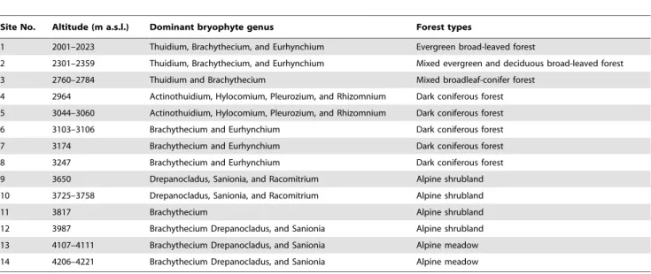
Table 3.Forest types and the most-prevalent bryophyte genus along the altitudinal gradient.
Site No. Altitude (m a.s.l.) Dominant bryophyte genus Forest types
1 2001–2023 Thuidium, Brachythecium, and Eurhynchium Evergreen broad-leaved forest
2 2301–2359 Thuidium, Brachythecium, and Eurhynchium Mixed evergreen and deciduous broad-leaved forest
3 2760–2784 Thuidium and Brachythecium Mixed broadleaf-conifer forest
4 2964 Actinothuidium, Hylocomium, Pleurozium, and Rhizomnium Dark coniferous forest
5 3044–3060 Actinothuidium, Hylocomium, Pleurozium, and Rhizomnium Dark coniferous forest
6 3103–3106 Brachythecium and Eurhynchium Dark coniferous forest
7 3174 Brachythecium and Eurhynchium Dark coniferous forest
8 3247 Brachythecium and Eurhynchium Dark coniferous forest
9 3650 Drepanocladus, Sanionia, and Racomitrium Alpine shrubland
10 3725–3758 Drepanocladus, Sanionia, and Racomitrium Alpine shrubland
11 3817 Brachythecium Alpine shrubland
12 3987 Brachythecium Drepanocladus, and Sanionia Alpine shrubland
13 4107–4111 Brachythecium Drepanocladus, and Sanionia Alpine meadow
14 4206–4221 Brachythecium Drepanocladus, and Sanionia Alpine meadow
even all trunks and branches are covered with dense bryophyte cushions.
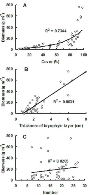
A clear humped relationship is observed between the bryophyte thickness and biomass and the elevation, with a maximum thickness of 8 cm and an averaged biomass of 700.3 g m22 around 3,758 m a.s.l. (Figure 2C, 2D). The biomass is very low (less than 50 g m22) between 2,001 and 2,784 m a.s.l., where the ecotones are evergreen broad-leaved forest, mixed evergreen and deciduous broad-leaved forest, and mixed broadleaf-conifer forest (Table 3). Higher biomass always coincided with both higher cover and higher thickness of bryophyte layer (Figure 2). Regression analysis also indicates that a significant exponential-relationship and a linear correlation are separately existed between bryophyte biomass and cover (p,0.05, Figure 3A), and between bryophyte biomass and bryophyte layer thickness (p,0.05, Figure 3B). Bryophyte biomass is unrelated to species number (Figure 3C).
Factors Influencing Bryophyte Species Composition and Distribution
According to CCA, depth of litter, air temperature, relative humidity and precipitation are the main factors correlated with bryophyte composition (Figure 4). The eigenvalues for the two first axes of the partial CCA are 0.720 and 0.395, respectively (Table 4). The first canonical axis explained 38.9%, the second 60.2%, and the first four axes 72.7% of the variation in species composition explained by the recorded explanatory variables. As shown in Figure 4, air temperature, and RH correlated to axis I, depth of litter and precipitation correlated with axis II. According to CCA, bryophytes can be categorized to 3 groups. For example, Actinothuidium, Hylocomiastrum, Hylocomium, Pleurozium, Pogonatum, Rhizomnium and Sphagnum are genus located in sites with higher RH and higher air temperature. Brachythecium, Bryhnia, Cirriphyllum, Eurhynchium, Mnium, Rhynchostegium, Taxiphyllum and Thuidium are genus growing in sites with higher litter depth. Bryonoguchia, Drepanocladus, Grimmia, Paraleuco-bryum, Ptilium, Racomitrium and Sanionia are genus growing in sites with higher precipitation.
Discussion
There is rich ground bryophyte diversity in Gongga Mountain, where 165 bryophyte species, including 42 liverworts and 123 mosses are found. Regions in the southwest of China are always rich in bryophytes, for example 153 bryophyte species including 118 mosses and 35 liverworts were reported in Xiaozhaizi Nature Reserve [51], and 134 mosses were reported in Wanglang Nature Reserve [52]. Rather, bryophytes in Gongga Mountain contribute greatly to the overall plant biodiversity in this region, and, even in Southwest China. However, we just investigated ground
bryo-Figure 3. Correlation analysis between bryophyte biomass and A) cover, B) thickness of bryophyte layer, and C) species number.
doi:10.1371/journal.pone.0058131.g003
Figure 4. CCA ordination Bio-plot for the most abundance bryophyte species. Genus abbreviation: Acti = Actinothuidium, Brac = Brachythecium, Bryh = Bryhnia, Bryo = Bryonoguchia, Cirr = Cirri-phyllum, Drep = Drepanocladus, Eurh = Eurhynchium, Grim = Grimmia, Hylo1 = Hylocomiastrum, Hylo2 = Hylocomium, Mniu = Mnium, Para = -Paraleucobryum, Pleu = Pleurozium, Pogo = Pogonatum, Ptil = Ptilium, Raco = Racomitrium, Rhiz = Rhizomnium, Rhyn = Rhynchostegium, Sa-ni = SaSa-nioSa-nia, Spha = Sphagnum, Taxi = Taxiphyllum, Thui = Thuidium;
Environment abbreviation: AT = Air temperature, LI = Depth of litter, PR = Precipitation, RH = Relative humidity.
phytes in this study, and broader investigations including other epiphytes types should be conducted later.
Although a clear humped relationship between the number of species and altitude below 3,650 m a.s.l., and an increasing trend above 3,650 m a.s.l. were observed, the elevation trend is highly curved from 2,001 m to 4,221 m a.s.l. This result differs significantly from those previous report in other places, where a decreasing trend [16], an increasing trend [12,17,18], or a hump-shaped distribution of species richness [15] were founded. In our study, the curved altitudinal trend of bryophyte species richness, especially the second increase trend following the first hump, is a new finding. In the present study, the humped relationship between species number and altitude stops at about 3,650 m a.s.l., the treeline of Gongga Mountain Forest. At this location, bryophyte community changes to genus dominated by Drepano-cladus, Sanionia, and Racomitrium, accompanying with the abrupt change of vegetation community from forest to open alpine shrubland. For the second increase of bryophyte diversity above 3,650 m a.s.l., one possible interpretation is the greater capacity of bryophytes to tolerate extreme conditions and the pioneer strategy of many bryophytes [18]. It could also be a part of a second hump which might appear if extended to higher altitudes. However, no investigation was conducted above 4,221 m a.s.l. in this study due to difficulty in accessing such sites.
The bryophyte distribution seems to be influenced by the elevation, and the bryophyte cover increases linearly with the increasing elevation. Vegetation types alternate along the altitu-dinal gradient (Table 3). From 2,001 to 2,358 m a.s.l., the vegetation are evergreen broad-leaved forest, and mixed evergreen and deciduous broad-leaved forests, where the ground bryophyte cover is low. From 2,964 to 3,987 m a.s.l., where the averaged bryophyte cover is higher than 85% with dark coniferous forest and alpine shrubland, and becomes an important vegetation layer. The terrestrial bryophyte cover linearly relates to elevation increase in Gongga Mountain, which is in accordance with the findings in tropical rain forests [53] and the Southern Appalachian Mountains [19].
The bryophyte biomass is linearly correlated with the thickness of bryophyte layer, exponentially correlated with the cover, but not correlated with the species number. In spite of this, higher biomass just appears at sites with both higher cover and higher thickness of bryophyte layer in this study (Figure 2). This kind of
relationship likely results from the difference of species composi-tion at different altitudes. For instance, pleurocarpous or creeping bryophytes generally have lower volume than the same cover of their acrocarpous or erect opponents. Therefore, large cover does not always mean a large biomass. However, a deep bryophyte layer thickness is commonly associated with particular species groups that often have large cover, which therefore produce a high biomass. Our result is in accordance with that provided by Kuusipalo [54], who developed bryophyte biomass models with two factors of percentage cover and height.
Results of CCA analysis suggests that the depth of litter, the air temperature, the precipitation and the relative humidity are the main factors influencing bryophyte species composition. One reason for the important role of air temperature, precipitation and the relative humidity in influencing bryophyte distribution might be the poikilohydric properties of bryophytes [10]. This result is in accordance with findings of Porley and Hodgetts [27], who explained that bryophyte distribution is influenced primarily by macroclimatic factors, including rainfall and temperature. Some other studies, suggesting that moisture is an important growth determinant more limiting than nutrients to bryophyte pro-ductivity [55], and that air temperature causes moss cover deterioration [56,57], also support our results.
The depth of litter is another major factor influencing terrestrial bryophyte distribution according to CCA results. Forests from 2,001 to 3,247 m a.s.l. are dominated by tall trees, where many rocks, fallen logs, branches, and twigs on the ground can grow the bryophytes [15]. Forests within the ranges of 2,001–2,358 m a.s.l. and 3,103–3,247 m a.s.l. are respectively dominated by tall broadleaves and conifers with dense undergrowth vegetation, where a thick layer of litter is formed. Bryophyte growth might be inhibited by shading and litter leachates [58–61]. Forests within the altitude range of 2,760–3,060 m a.s.l. are dominated by mixed broadleaved-conifer or conifers with few shrubs only, where fallen branches and twigs provide a favorable substrate for the inhabitation of bryophytes but without the limitation of litter thickness. At altitudes higher than 3,650 m a.s.l., close to the timber line (approximately 3,600 m in Gongga Mountain), fallen branches and twigs are rare. With increasing altitude, the vegetation changes gradually into alpine meadow. The herbaceous vegetation and its litter have good moisture-holding capacity and Table 4.Results of the CCA, showing eigenvalues, cumulative explained variance of species data, species–environment correlation coefficients, and correlation coefficients of the environmental variables for the 4 axes established.
Axes F P
1 2 3 4
Eigenvalues 0.720 0.395 0.143 0.089
Species-environment correlations 0.969 0.875 0.864 0.737
Cumulative percentage variance
of species data 38.9 60.2 67.9 72.7
of species-environment relation 53.4 82.7 93.4 100.0
Environmental variables correlation coefficients
AT 0.6982 0.176 0.5713 20.0441 9.120 0.0010
RH 0.7924 20.2129 0.2557 20.3168 16.19 0.0010
PR 20.2446 20.2874 0.4881 20.5261 15.54 0.0010
LI 0.6359 0.6515 20.0199 0.0893 18.99 0.0010
nutrient availability at this region, and therefore benefit for bryophyte species [62].
Conclusions
Our investigations show the rich terrestrial bryophyte diversity in Gongga Mountain. A clear humped relationship between the amount of species and the elevation below 3,650 m a.s.l., as well as an increasing trend above 3,650 m a.s.l. are found. From 2,001 to 4,221 m a.s.l, the species richness increases in a high curvature trends. These features significantly differ from those of previous investigations, especially the second increase trends following the first hump in our investigation.
The cover of terrestrial bryophyte increases with elevation, while the biomass and the thickness of bryophyte exhibit a clear humped relationship with the elevation. The elevation of 3,758 m a.s.l. is a key point for bryophytes, where the averaged biomass of 700.3 g m22 and the maximum thickness of 8 cm are observed. These results are helpful for modeling ecosystem carbon and nutrient cycling, as well as promoting the understanding of bryophytes’ ecological role in the forest ecosystem.
The bryophyte distribution is primarily associated with the depth of litter, the air temperature and the precipitation. The
relationship between bryophyte distribution and climatic proxies might be useful for modeling responses of bryophyte to climate changes. However, in this study, just ground bryophytes were investigated, and no sites above 4,221 m a.s.l. were examined.
Supporting Information
Table S1.
(DOC)
Acknowledgments
We specially thank Prof. Tong Cao in Shanghai Normal University, Shanghai, China, for his assistance in bryophyte species identification. We also thank Prof. Graham Shields from University College London for his assistance in English corrections.
Author Contributions
Conceived and designed the experiments: SQS GXW. Performed the experiments: SQS JZ DY. Analyzed the data: YHW HJB. Contributed reagents/materials/analysis tools: JL. Wrote the paper: SQS.
References
1. Grytnes JA, Heegaard E, Ihlen PG (2006) Species richness of vascular plants, bryophytes and lichens along an altitudinal gradient in western Norway. Acta Oecol 29: 241–246.
2. Ingerpuu N, Vellak K, Kukk T, Pa¨rtel M (2001) Bryophyte and vascular plant species richness in boreo-nemoral moist forests and mires. Biodivers Conserv 10: 2153–2166.
3. Steel JB, Wilson JB, Anderson BJ, Lodge RHL, Tangney RS (2004) Are bryophyte communities different from higher-plant communities? Abundance relations. Oikos 104: 479–486.
4. Frego KA (2007) Bryophytes as potential indicators of forest integrity. Forest Ecol Manag 242: 65–75.
5. Jeschke M, Kiehl K (2008) Effects of a dense moss layer on germination and establishment of vascular plants in newly created calcareous grasslands. Flora 203: 557–566.
6. Belnap J, Bu¨del B, Lange OL (2003) Biological soil crusts: characteristics and distribution. In: Belnap J, Lange OL, editors. Ecological Studies 150: Biological soil crusts: Structure, function, and management. Berlin, Heidelberg, New York: Springer. 3–30.
7. Zhao J, Zheng Y, Zhang B, Chen Y, Zhang Y (2009) Progress in the study of algae and mosses in biological soil crusts. Frontiers of Biology in China 4: 143– 150.
8. Turetsky MR (2003) The role of bryophytes in carbon and nitrogen cycling. Bryologist 106: 395–409.
9. Beringer J, Lynch AH, Chapin FS, Mack M, Bonan GB (2001) The representation of arctic soils in the land surface model: the importance of mosses. J Climate 14: 3324–3335.
10. Uchida M, Muraoka H, Nakatsubo T, Bekku Y, Ueno T, et al. (2002) Net photosynthesis, respiration, and production of the moss Sanionia uncinata on a glacier foreland in the high arctic, Ny-Alesund, Svalbard. Arct Antarc Alp Res 34: 287–292.
11. Delach A, Kimmerer RW (2002) The effect of Polytrichum piliferum on seed germination and establishment on iron mine tailings in New York. Bryologist 105: 249–255.
12. Ah-Peng C, Chuah-Petiot M, Descamps-Julien B, Bardat J, Stamenoff P, et al. (2007) Bryophyte diversity and distribution along an altitudinal gradient on a lava flow in La Re´union. Divers Distrib 13: 654–662.
13. Andrew NR, Rodgerson L, Dunlop M (2003) Variation in invertebrate-bryophyte community structure at different spatial scales along altitudinal gradients. J Biogeogr 30: 731–746.
14. Gignac LD (2001) Bryophytes as Indicators of climate change.Bryologist104:
410–420.
15. Grau O, Grytnes J, Birks HJB (2007) A comparison of altitudinal species richness patterns of bryophytes with other plant groups in Nepal, Central Himalaya. J Biogeogr 34: 1907–1915.
16. Tusiime FM, Byarujali SM, Bates JW (2007) Diversity and distribution of bryophytes in three forest types of Bwindi Impenetrable National Park, Uganda. Afr J Ecol 45: 79–87.
17. Frahm JP, Ohlemu¨ller R (2001) Ecology of bryophytes along altitudinal and latitudinal gradients in New Zealand. Studies in austral temperate rain forest bryophytes 15. Trop Bryol 20: 117–137.
18. Bruun HH, Moen J, Virtanen R, Grytnes JA, Oksanen L, et al. (2006) Effects of altitude and topography on species richness of vascular plants, bryophytes and lichens in alpine communities. J Veg Sci 17: 37–46.
19. Stehn SE, Webster CR, Glime JM (2010) Elevational gradients of bryophyte diversity, life forms, and community assemblage in the southern appalachian mountains. Can J Forest Res 40: 2164–2174.
20. Ma´rialigeti S, Ne´meth B, Tinya F, O´ dor P (2009) The effects of stand structure
on ground-floor bryophyte assemblages in temperate mixed forests. Biodivers Conserv 18: 2223–2241.
21. Weibull H, Rydin H (2005) Bryophytes species richness on boulders: relationship to area, habitat diversity and canopy tree species. Biol Conserv 122: 71–79. 22. Shields JM, Webster CR, Glime JM (2007) Bryophyte community response to
silvicultural opening size in a managed northern hardwood forest. Forest Ecol Manag 252: 222–229.
23. Bardat J, Aubert M (2007) Impact of forest management on the diversity of corticolous bryophyte assemblages in temperate forests. Biol Conserv 139: 47– 66.
24. Bergamini A, Ungricht S, Hofmann H (2009) An elevational shift of cryophilous bryophytes in the last century–an effect of climate warming? Divers Distrib 15: 871–879.
25. Ja¨gerbrand AK, Alatalo JM, Chrimes D, Molau U (2009) Plant community responses to 5 years of simulated climate change in meadow and heath ecosystems at a subarctic-alpine site. Oecologia 161: 601–610.
26. Pharo EJ, Beattie AJ (2002) The association between substrate variability and bryophyte and lichen diversity in eastern Australian forests. Bryologist 105: 11– 26.
27. Porley R, Hodgetts N (2005) Mosses and Liverworts. Harper Collins Publishers, London, UK.
28. Pentecost A (1998) Some observations on the biomass and distribution of cryptogamic epiphytes in the upper montane forest of the Rwenzori mountains, Uganda. Global Ecol Biogeogr Lett 7: 273–284.
29. Batty K, Bates JW, Bell JNB (2003) A transplant experiment on the factors preventing lichen colonization of oak bark in South-east England under declining sulphurdioxide pollution. Can J Bot 81: 439–451.
30. Vellak K, Paal J, Liira J (2003) Diversity and distribution pattern of bryophytes and vascular plants in a boreal spruce forest. Silva Fenn 37: 3–13.
31. Huo C, Cheng G, Lu X, Fan J (2010) Simulating the effects of climate change on forest dynamics on Gongga Mountain, Southwest China. J Forest Res 15: 176– 185.
32. Fernando TM, Cristina E, Isabel M, Adria´n E (2008) Are soil lichen communities structured by biotic interactions? A null model analysis. J Veg Sci 19: 261–266.
33. Gao Q (1994a) Flora bryophytorum sinicorum. I. Sphagnales andreaeales, Archidiales dicranales. Science Press, Beijing, China.
34. Gao Q (1994b) Flora bryophytorum sinicorum. II. Fissidentales, Pottiales. Science Press, Beijing, China.
35. Li XJ (2000) Flora bryophytorum sinicorum. III. Grimmiales, Funariales, Tetraphidales. Science Press, Beijing, China.
37. Wu PC (2002) Flora bryophytorum sinicorum. VI. Dedicatum. Science Press, Beijing, China.
38. Hu RL, Wang YF (2005) Flora bryophytorum sinicorum. VII. Hypnobryales. Science Press, Beijing, China.
39. Wu PC, Jia Y (2004) Flora bryophytorum sinicorum. VIII. Hypnobryales, Buxbaumiales, Polytrichales, Takakiales. Science Press, Beijing, China. 40. Gao Q (2003) Flora bryophytorum sinicorum. IX. Takakiales, Calobryales,
Jungermanniales. Science Press, Beijing, China.
41. Gao Q, Wu YH (2008) Flora bryophytorum sinicorum. X. Jungermanniales (Lophoziaceae-Neotrichocoleaceae). Science Press, Beijing, China.
42. Gao Q, Lai MZ (2003). Illustrations of bryophytes of China. SMC publishing Inc, Taibei.
43. O’Shea BJ (2003) Checklist of the mosses of sub-Saharan Africa. (version 4, 12/ 03). Tropical Bryology Research Reports 4: 1–176.
44. Wigginton MJ (2004) Checklist and distribution of the liverworts and hornworts of Sub-Saharan Africa, including the East African Islands (edition 2, September 2004). Tropical Bryology Research Reports 5: 1–102.
45. Mandl NA, Kessler M, Gradstein SR (2009) Effects of environmental heterogeneity on species diversity and composition of terrestrial bryophyte assemblages in tropical montane forests of southern Ecuador. Plant Ecol Divers 2: 313–321.
46. Swartaman G, Huang C, Kaluzny S (1992) Spacial analysis of Bering Sea groundfish survey data using generalized addictive models. Can J Fish Aquat Sci 49:1366–1378.
47. Insightful Corp (2007) Insightful S-Plus 8.0. Insightful Corp, Seattle, Washing-ton.
48. Ter Braak CJF, Smilauer P (1998) CANOCO reference manual and user’s guide to CANOCO for windows, Software for canonical community ordination (Version 4). Microcomputer Power, New York.
49. Lepsˇ J, Sˇmilauer P, 2003. Multivariate analysis of ecological data using CANOCO. Cambridge University Press, Cambridge, United Kingdom. 50. Ter Braak CJ, milauer P (2002) CANOCO Reference Manual and CanoDraw
for Windows User’s Guide: Software for Canonical Community Ordination (Version 4.5). Microcomputer Power, Ithaca, NY.
51. Wang CB, Zhang W, He XJ (2007) Investigation and Analysis on the Resources of Bryophyte in Xiaozhaizi Nature Reserve of Sichuan Province. Chinese Wild Plant Resources 26: 35–37.
52. Li ZH, Yu J, Cao T, Li Q (2010) A first report of the mosses from Wanglang Nature Reserve, Sichuan Province, China. Journal of Guizhou Normal University (Natural Sciences). 28: 156–161.
53. Frahm JP, Gradstein SR (1991) An altitudinal zonation of tropical rain forests using byrophytes. J Biogeogr 18: 669–678.
54. Kuusipalo J (1983) Mustikan varvuston biomassama¨a¨ra¨n vaihtelusta erilaisissa metsiko¨issa¨. Silva Fennica 17: 245–257.
55. Skre O, Oechel WC (1981) Moss functioning in different taiga ecosystems in interior Alaska. I. Seasonal, phenotypic, and drought effects on photosynthesis and response patterns. Oecologia 48: 50–59.
56. Jo´nsdo´ttir IS, Magnu´sson B, Gudmundsson J, Elmarsdo´ttir A´ , Hjartarson H
(2005) Variable sensitivity of plant communities in Iceland to experimental warming. Global Change Biol 11: 553–563.
57. Walker MD, Wahren CH, Hollister RD, Henryd GHR, Ahlquist LE, et al. (2006) Plant community responses to experimental warming across the tundra biome. PNAS 103: 1342–1346.
58. Corrales A, Duque A, Uribe J, London˜o V (2010) Abundance and diversity patterns of terrestrial bryophyte species in secondary and planted montane forests in the northern portion of the Central Cordillera of Colombia. Bryologist 113: 8–21.
59. Virtanen R, Crawley MJ (2010) Contrasting patterns in bryophyte and vascular plant species richness in relation to elevation, biomass and Soay sheep on St Kilda, Scotland. Plant Ecol Divers 3: 77–85.
60. Peintinger M, Bergamini A (2006) Community structure and diversity of bryophytes and vascular plants in abandoned fen meadows. Plant Ecol 185: 1– 17.
61. Startsev N, Lieffers VJ, Landha¨usser SM (2008) Effects of leaf litter on the growth of boreal feather mosses: implication for forest floor development. J Veg Sci 19: 253–260.