Mile Petkovski, Mitko Kostov, Ramona Markoska, Aleksandar Markoski, (2013). DWT Coefficients Estimation in Images with Missing Samples, TEM Journal, 2(4), pp. 277-282.
DWT Coefficients Estimation in Images with
Missing Samples
Mile Petkovski
1, Mitko Kostov
1, Ramona Markoska
1, Aleksandar Markoski
11
Faculty of Technical Sciences, St. Kliment Ohridski University, Bitola, Macedonia
Abstract – In this paper we propose a procedure for discrete wavelet transform coefficients estimation on the images with missing samples. This procedure extends application of multiresolutionally based algorithm for non-uniformly sampled signal reconstruction. Estimation efficiency is tested on proprietary chosen images and results are presented graphically.
Keywords – Discrete wavelet transform, missing samples.
1. Introduction
Digital images, produced to record or display useful information, are becoming an important way of communication. However, digital images may be distorted and degraded during image formation, acquisition, storage or transmission. In the process of capturing an image, due to detector malfunction or some other reasons, it is not uncommon that some of the pixel values are not recorded. In some cases, missing regions in an image are due to transmission errors. This leads to loss of image quality, consequently the degraded image needs processing before it can be used in applications. Therefore, image restoration is an important issue in high-level image processing with purpose to estimate the original image from the degraded data.
One approach to processing images is to use an image decomposition that is expected to be sparse, like the wavelet transform [1, 2]. Some variations of the wavelet transform decomposition techniques contribute to its efficiency in signal processing [3]. The wavelet transform adapts to spatial and frequency in-homogeneities and therefore it has been successfully used in several image processing applications. However, in the case of images with missing pixels, the presence of unobserved pixel values prevents the existing wavelet techniques to be directly applied to recover the original image. Complexity of the problem arises from samples with unknown locations [4]. There are a many developed reconstruction algorithms established on different basis functions as multiresolutional spline solution [5], Fourier base functions [6] and wavelets [7, 8].
In this paper we describe an approach to image recovery when images miss pixels. The basic idea is to extend existing multiresolutionaly based
algorithms for non-uniformly sampled signal reconstruction [7], and improved version [8], applying conjugate gradient method [9, 10] for solving linear system of equations. Considering an image with missing regions, we investigate the problem of estimating its wavelet coefficients and then apply inverse wavelet transform. The main goal of the paper is to show that estimation of the discrete wavelet coefficients give some advantages to perform some additional processing like compression and/or noise reduction in the phase of image reconstruction.
The paper is organized as follows. Section 2 presents required theoretical background for algorithm development, section 3. Experimental results over proprietary chosen image are presented in section 4. Section 5 comments some of properties of proposed algorithm.
2. Theoretical Fundamentals
2.1. Discrete Wavelet Transform
In series expansion of discrete-time function f
using wavelets.
∑
∑
∑
= = =
− −
+ = J
j
M
k
Jk Jk M
k
jk jk
J j
t a t
d t
f
1
2
1 2
1
) ( )
( )
(
ψ
φ
(1)ψjk and φjk denote wavelet and scaling function,
respectively, the indexes j and k are for dilatation and translation, and aJk and djk are approximation and
detail coefficients [1].
Wavelet decompositions and multiresolution concepts are closely related to filter bank theory. For this reason, it is helpful to view the scaling and wavelet function as a low pass and high pass filter, h0
and h1, respectively. The wavelet transform is
applied to low pass results (approximations) only as it is illustrated in Fig. 1.
∑
−
=
n
n
t
h
t
)
2
(
2
)
(
1/2 1ψ
ψ
(2)∑
−
=
n
n
t
h
t
)
2
(
2
)
(
1/2 0φ
2.2. Two Dimensional Discrete Wavelet Transform
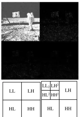
Discrete wavelet transform (DWT) can be applied to an image in two ways: by applying 2D wavelets or by computing 1D wavelet transform of the image by alternating between rows and columns. In the later method, the first step is to apply 1D wavelet transforms to all the rows (or columns) by using lowpass and highpass filters. The standard algorithm then computes the wavelet transform of every column (or row) by using the same filters (Fig. 2). The first step of the whole process is summarized in Fig. 3. On the left, the well-known image Moon is shown. To the right, 1D wavelet transform to the columns of the image is applied. The corresponding result is composed of a coarse and scaled version of the original and the details. This interpretation is illustrated as low and high frequency coefficients blocks, denoted by L and H, respectively. Next, the transform is applied to the rows of the already vertically transformed image as well. The result is shown in Fig. 4 and is decomposed into four quadrants with different interpretations.
The horizontal and vertical details of the image are highlighted in the quadrants HL and LH. These blocks were filtered along the rows and columns by the low pass filter h0 and the high pass filter h1,
alternatively. The quadrant HH represents the diagonal details of the image obtained by filtering the image with the use of the filter h1. The quadrant LL
represents the trend values obtained by filtering the image with the filter h0.
Next, 2D wavelet transform can be iterated on the coarser version at half the resolution, recursively, as it is illustrated in Fig. 4c.
H0 2
H1 2
f =a0,k
d1,k
a1,k
H0 2
H1 2 d2,k
a2,k
. . .
H0 2
H1 2 dJ,k
aJ,k
a1,k
Figure 1. Discrete wavelet transform tree.
H0 2
H1 2
x[m,n]
v1,H[m,n]
H0 2
H1 2
H0 2
H1 2
along n
along n
v1,L[m,n]
along m
along m
along m
along m
x1,LL[m,n]
x1,LH[m,n]
x1,HL[m,n]
x1,HH[m,n]
Figure 2. Schematic diagram of 2D wavelet transform.
LL
HL
LH
HH
LL2
HL2
LH2
HH2
HL
LH
HH
Figure 4. One dimensional discrete wavelet transform applied to the rows of the already vertically
transformed image Moon.
L
H
2.3. Discrete Least Square Approximation
In many situations interpolation is not warranted. Errors in the data, smoothness constraints, data compression, local control, computational cost, physical , etc. are all reasons for allowing the approximating function to pass “near” - rather than “through” - the data.
This data-fitting, or curve-fitting, is fundamentally an optimization problem: “What is the ‘best’ approximating function (from some fixed set) for this data?”. Two things need to be decided for this problem to be well defined. First, what class of function is one considering? Polynomials, trigonometric functions, wavelets, exponential functions, splines, and eigenfunctions associated with some related operator, are all examples of classes of functions commonly used in this context. Second, what does one mean by “best”? Here the best will minimize the sum of the squares of the (vertical) error (
2
⋅ minimization), but there are as many reasonable definitions of “best” for a given application as there are reasonable measures of distance for that application.
On the other hand, if we are given the data
(
x y1, 1) (
, x y2, 2)
,(
x yn, n)
, and we let[
1, 2,]
T n
x= x x x and y=
[
y y1, 2,yn]
T,then the discrete least squares solution for this data is a function
( )
(
)
2 1/ 2 1arg min
n
i i
g S i
f
y
g x
∈ =
=
−
∑
(4)In general, this can be an arbitrarily difficult problem (e.g. if
S
is a large discrete set), but ifS
is a vector space then this linear least squares problem is much more simple, in fact we can do the finite dimensional case right here: Letφ φ
1,
2,
,
φ
n be any basis forS
and letV
be the m n× matrix( )
j i
V =
φ
x (this is a bit different for thecontinuous case).
Then
1
m
i i i
f
c
φ
=
=
∑
, where2
arg min
m
c∈
=
c
y - Vc
R (5)
the solution to the minimization problem above uniquely satisfies the normal equations
T T
V Vc = V y
(6)It is well known that the coefficients in a least squares fit for a given set of data points are found by
“solving” an overdetermined system of linear equations. The vector of coefficients can be found by applying the pseudoinverse of the matrix of coefficients. ln this paper we explore an overdetermined system of linear equations to find an appropriate “best solution." Much of the general theory of least squares fit is arrived at from a different point of view.
Consider a system of linear equations
Ax = b
(7)where A is an m n× matrix of rank n, with
m>n. The picture is
11 1 1
1
1
n
n
m mn n
a
a
b
x
x
a
a
b
=
(8)Such a system is said to be overdetermined. In general such a system will have no solution. Let us solve this system as “best we can." A is not a square matrix. There is thus no possibility of multiplying both sides of the equation (7) by the inverse of A to get
x
. However we can modify the equation so thatx
can be isolated.Multiply both sides of the equation by
A
T to getT
=
TA Ax
A b
(9)Note that
A A
T a square n n× matrix. The rankof
A A
T is known to be the same as the rank ofA.Thus
(
A AT)
−1 exists. Multiply both sides of thisequation by
(
A AT)
−1 to isolatex
, we get(
T) (
−1 T)
=
x A A A A b (10)
(
T)
−1 TA A A is called the pseudoinverse of Α, and
x
is called the least square solution of the system (7). More formally, we find a vectorx
*such that2 2
≤
*
Ax - b
Ax - b
(11)2.4. The Conjugate Gradient Method (CG)
The Conjugate Gradient method is an effective method for symmetric positive definite systems,
Ax = b
, and proceeds by generating vector sequences (i.e., successive approximations to the solution), residuals corresponding to the iterates, and search directions used in updating the iterates and residuals. In each iteration i the iterates x( )
i areupdated by a multiple i of the search direction p
( )
i) ( ) 1 ( ) ( i i i i ap x
x = − + (12)
The corresponding residuals
r
(i)=
b
−
Ax
(i) are updated as ) ( ) 1 ( ) ( i i i i aq rr = − + (13)
where
q
(i)=
Ap
(i). The choice:) ( T ) ( ) 1 ( T ) 1 ( i i i i i
Ap
p
r
r
− −=
α
(14)minimizes
r
(i)TA
−1r
(i) over all possible choices forai. The search directions are updated using the
residuals: ) 1 ( 1 ) ( ) ( − − + = i i i i b p r p (15)
where the choice:
) 1 ( T ) 1 ( ) ( T ) ( − −
=
i i iii
r
r
r
r
β
(16)ensures that
p
(i) andAp
(i−1), (or equivalentlyr
(i)and
r
(i−1) are orthogonal. Convergence is achieved in at most n steps of iteration, where n is the dimension of the system.3. Algorithm Development
3.1. Description of the problem
Images with missing samples are considered as a set of columns and/or rows with missing samples, i.e. many one dimensional signals. The existing pixels are treated as non- uniformly distributed samples of the signal. Our goal is to find an estimation of discrete wavelet transform coefficients of every column, approximation and details.
We assume that the non-uniformly sampled signal is under-sampled with respect to the Nyquist frequency of the complete uniformly sampled signal.
3.2. Estimation of DWT coefficients
Suppose that the non-uniformly sampled data y has been obtained through sub-sampling of the signal x, as expressed by the following equation:
Y = HSx (17)
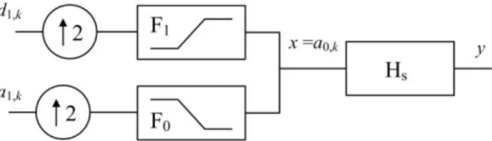
where HS consisting of entries 1 and 0 is so called a sub-sampling matrix. The discrete wavelet coefficients estimation procedure starts from first resolution level, depicted on Fig 5.
Since we do not have all of the samples on the desired grid, we cannot compute the wavelet coefficients of the signal. However, we can estimate approximation coefficients of the signal by its low frequency components, temporarily ignoring the high-frequency terms. These assumptions produce the predetermined linear system:
( )
a y FHS 0 ↑2 1 = (18)
We are looking for a least-squares approximation to this system. Since the system of equations is ill conditioned a method of conjugate gradients is applied as a suitable tool solving the system with minimum iteration steps. The scaling function coefficients, represented by vector a1, are estimated
by applying the method of conjugate gradients in the approximation procedure. The estimates a’1 yield a
low frequency estimate x’ denoted by x’a:
( )
'1 0'
2a F
xa = ↑ (19)
In the next step, we calculate the error signal at each available sample:
a
x H y
e1 = − S ' (20)
Similarly as above, we can estimate the detail coefficients of the first level decomposition by solving the predetermined linear system:
( )
1 11
2
d
e
F
H
S↑
=
(21)By solving this predetermined system we estimate the detail coefficients d’1.
Since the matrices that appear in previously defined pre-determined linear systems of equations contain a significant number of zero-valued elements, by applying sparse matrix techniques, the computational time and the number of floating point operations are reduced significantly.
3.3. Estimation of DWT2 coefficients
Discrete wavelet transform coefficients estimation procedure described in the previous subsection is performed to the every column of the image with missing samples. Thus computed vectors are placed instead of older image columns. This leads to matrix similar to image shown in Fig. 3. This matrix represents the low and high frequency coefficient blocks. To the already estimated coefficients of vertically transformed image the discrete wavelet transform is applied to the rows with intention to obtain four-quadrant image with estimated DWT2 coefficients.
4. Experimental Results
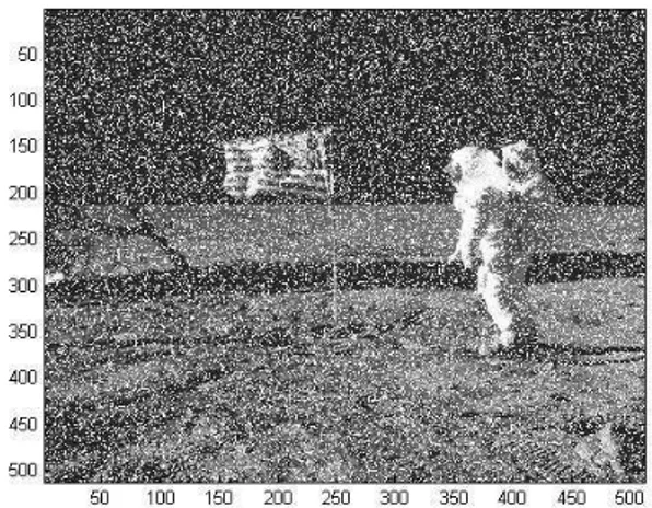
As a test signal a 512 x 512 resolution image is exploited. Randomly chosen pixels are omitted and picture with missing pixels is presented on the Fig.6. In the experiment 25% of pixels in the entire image are missing.
Algorithm starts from the first column of image, estimating approximation and detail coefficient of its discrete wavelet transform. Such computed coefficient vectors are merged and take place on the
corresponding column with missing samples in the image on Fig. 7. The upper rows represent approximation, i.e. low frequency block and lower rows represent details coefficients.
Recently obtained image is further processed applying discrete wavelet transform on every row and results are presented on the Fig.8, showing estimated discrete wavelet transform coefficients of image with missing samples. The upper left part presents approximation coefficients and lower right diagonal details. The other two parts presents the estimation of horizontal and vertical wavelet transform coefficient.
Performing inverse discrete wavelet transform on the estimation presented at Fig. 8, the reconstructed image is obtained and presented on the Fig. 9.
5. Conclusion
We have proposed an approximation technique applied to estimate the 2D discrete wavelet transform coefficients. This algorithm generates discrete wavelet transform coefficients in a form suitable for further processing before reconstruction phase of the
Figure 6. Image with missing pixels.
Figure 7. First stage of estimation procedure.
signal, such as compression and denoising. Results slightly differ using different wavelet basis.
It is obvious that utilizing this reconstruction techniques many details in the original image are successfully reconstructed, some details on the flag and spaceship, and especially footprints in the surface which cannot be recognized on the image with missing samples.
6. References
[1]. G. Strang and T. Nguyen, Wavelets and Filter Banks, Wellesley-Cambridge Press, Wellesley MA, 1995. [2]. M. Vetterli and J. Kovacevic, Wavelets and Subband
Coding, Prentice Hall, NJ 1995.
[3]. I. Ram, M. Elad, I. Cohen, “Generalized Tree-Based Wavelet Transform”, IEEE Trans. Signal Processing,
vol. 59, No. 9, pp. 4199-4209 September 2011.
[4]. P. Marziliano, M. Vetterli,”Reconstruction of Irregularly Sampled Discrete-Time Bandlimited Signals with Unknown Sampling Locations”, IEEE Trans. Signal Processing, vol. 48, No. 12 Dec. 2000 [5]. M. Arigovindan, M. Sühling, P. Hunziker, M.
Unser, “Variational Image Reconstruction From Arbitrarily Spaced Samples: A Fast Multiresolution Spline Solution”, IEEE Trans. Image Proc., Vol. 14 No.4, pp. 450-460, 2005
[6]. T. Strohmer, “Computationally attractive recon-struction of band-limited images from irregular samples”, IEEE Trans. Image Proc., Vol. 6 No.4, pp. 540-548, 1997.
[7]. Ford C. and Etter D.M, “Wavelet basis reconstruction of nonuniformly sampled data,” IEEE Trans. Circuits Syst. IIl, vol. 45(8), pp. 573–576, 1995.
[8]. M. Petkovski and M. Bogdanov, “Estimation of discrete wavelet transform coefficients of non-uniformly sampled signals,” Proc. Int. Symp. on Signals, Circuits and Systems, SCS 2001, pp. 9–14, July.
[9]. Chan T.F. Demmel J. Donato J. Dongarra J. Eijkhout V. Pozo R. Romine C. Barret R., Berry M. and Van der Vorst H, “Templates for the solution of linear systems: Building blocks for iterative methods,” SIAM Press, 1994.
[10].David Kincaid and Ward Cheney, Numerical Analysis, Brooks/Cole Publishing Company, Belmont, CA, 1991.
Corresponding author: Mile Petkovski
Institution: Faculty of Technical Sciences Bitola, Macedonia
E-mail: [email protected]