EVALUATION OF WAVELET DENOISING METHODS FOR SMALL-SCALE JOINT
ROUGHNESS ESTIMATION USING TERRESTRIAL LASER SCANNING
M. Bitenc a,*, D. S. Kieffer a, K. Khoshelhamb
a
Institute of Applied Geosciences, Graz University of Technology, Austria - (bitenc, kieffer)@tugraz.at b
Department of Infrastructure Engineering, The University of Melbourne, Victoria 3010, Australia – k.khoshelham@unimelb.edu.au
Commission VI, WG VI/4
KEY WORDS: terrestrial laser scanning, joint roughness, range noise, discrete wavelet transform, stationary wavelet transform, denoising performance
ABSTRACT:
The precision of Terrestrial Laser Scanning (TLS) data depends mainly on the inherent random range error, which hinders extraction of small details from TLS measurements. New post processing algorithms have been developed that reduce or eliminate the noise and therefore enable modelling details at a smaller scale than one would traditionally expect. The aim of this research is to find the optimum denoising method such that the corrected TLS data provides a reliable estimation of small-scale rock joint roughness. Two wavelet-based denoising methods are considered, namely Discrete Wavelet Transform (DWT) and Stationary Wavelet Transform (SWT), in combination with different thresholding procedures. The question is, which technique provides a more accurate roughness estimates considering (i) wavelet transform (SWT or DWT), (ii) thresholding method (fixed-form or penalised low) and (iii) thresholding mode (soft or hard). The performance of denoising methods is tested by two analyses, namely method noise and method sensitivity to noise. The reference data are precise Advanced TOpometric Sensor (ATOS) measurements obtained on 20×30 cm rock joint sample, which are for the second analysis corrupted by different levels of noise. With such a controlled noise level experiments it is possible to evaluate the methods’ performance for different amounts of noise, which might be present in TLS data. Qualitative visual checks of denoised surfaces and quantitative parameters such as grid height and roughness are considered in a comparative analysis of denoising methods. Results indicate that the preferred method for realistic roughness estimation is DWT with penalised low hard thresholding.
1. INTRODUCTION
In the last few decades Terrestrial Laser Scanning (TLS) is increasingly used in the field of engineering geology for a growing array of applications (Fowler, 2011; Fernández-Steeger et al., 2009). Because of remote and fast acquisition that results in relative high resolution and accuracy data, TLS is valuable for in-situ rock mass characterization (Tonon and Kottenstette, 2006); especially for estimating geometrical parameters (Slob, 2010). One of them is rock joint roughness, which significantly influences rock mass stability, and for this reason needs to be precisely estimated for each engineering project.
Rock joint roughness describes the morphology of joint surfaces (roughness amplitude) in certain direction and at certain scales. Roughness direction should be consistent with expected rock mass movements (shear direction). When the shear direction is not known a-priori, roughness should be measured in all possible directions. Roughness scale dependency was attributed to sample size (Barton and Choubey, 1977), but the studies, which are summarized in (Tatone and Grasselli, 2012), show contradictory results. In case of large discontinuities, the joint roughness consists of large-scale (waviness or primary roughness) and small-scale (unevenness or secondary roughness) components (ISRM, 1978). Waviness can be described as a large-amplitude and low-frequency signal. It has been defined by (Priest, 1993) as “surface irregularities with a wavelength greater than about 10 cm”. Unevenness can be described as a small-amplitude and high-frequency signal. It covers finer scales of 5 to 10 cm and is superimposed on the waviness.
Due to historical reasons, including limited amount of 1D or 2D surface measurements and low computational power, roughness is traditionally parameterized by a single value as e.g. Joint Roughness Coefficient (JRC) (Barton, 1973) or dilation angle (Patton, 1966). Taking profile measurements rather than considering 3D surface topography can lead to biased estimates of roughness as for example explained in (Rasouli and Harrison, 2004). Therefore newer studies took advantage of available 3D remote sensing data and developed new roughness parameters such as fractals (e.g. Fardin, 2004) or the angular threshold method (Grasselli, 2001). Nevertheless, those parameters have limited ability to describe the three attributes of roughness, namely amplitude, direction and scale dependency. A combination of precise and dense 3D measurements of in-situ large scale rock joints and truly 3D roughness parameters would improve rock mass stability analysis and better support engineering geologist decisions. In our research the efficacy of TLS as a means for in-situ characterization of joint surfaces is investigated.
Sturzenegger and Stead (2009) stated that TLS technology and careful fieldwork allow the extraction of first-order roughness profiles, but for the secondary roughness estimation the raw TLS point clouds do not fully satisfy requirements for data resolution and accuracy. TLS data resolution refers to the ability to resolve two objects on adjacent sight lines and depends on sampling interval (nominal point spacing) and laser beamwidth (footprint size) (Lichti and Jamtsho, 2006). The smallest resolution is therefore defined by laser scanner capability to steer the laser beam for small angular increments and to focus the laser beam in a small footprint. Because the footprint size depends on scanning geometry (the range and incidence angle),
it is generally advised to scan a surface as close as possible and optimally in perpendicular direction. The resulting (effective) TLS data resolution, which was studied in (Lichti and Jamtsho, 2006; Pesci et al., 2011), defines the smallest size of observable feature, this is the smallest roughness scale. TLS data accuracy depends on several factors: (i) imprecision of laser scanner mechanism, (ii) geometric properties of scanned surface, this is scanning geometry, (iii) physical properties of scanned surface material and (iv) environmental (atmospheric) conditions (Soudarissanane et al., 2011). Resulting measurement errors are composed of systematic and random errors. Systematic errors are usually removed by a proper calibration procedure (Lichti, 2007). The remaining random errors, which are attributed mainly to range error and are therefore referred to as range noise, are in order of a few millimetres. An appropriate denoising method would improve capabilities of TLS for modelling small-scale details.
Advances in computer technology have enabled development of fast and efficient post-processing algorithms that reduce or ideally eliminate noise in TLS data and at the same time preserve surface details. Existing methods to estimate and eliminate TLS range noise include empirical methods, where reference data of higher accuracy or a known reference model are used, interpolation methods using simple averaging or more elaborate smoothing functions, and theoretical methods based on error propagation models. Interpolation methods are commonly used since no additional data or assumptions are needed with respect to reference data or a theoretical model. Inputs for those denoising methods are either 3D point clouds or 2.5D surfaces. A short list of 3D point cloud or mesh methods is given in (Smigiel et al., 2008). Commonly the complexity of a 3D randomly scattered point cloud is reduced by gridding. Having Cartesian coordinates (x,y,z), a grid of certain cell size is constructed in the chosen two directions and the third coordinate is assigned to each grid point. Another approach for obtaining a 2.5D surface was used by Smigiel et al. (2008). They transformed Cartesian coordinates to polar coordinates (horizontal and vertical angle, and range), which are actually TLS original measurements, and computed the so-called range image. An advantage of 2.5D surface is that a whole range of existing image processing algorithms can be used. An overview of image denoising methods and further references can be found in (Buades et al., 2005; Smigiel et al., 2011; Zhang et al. 2014).
An objective of image denoising methods is to decompose smooth and oscillatory part. Therefore, image filtering techniques result in data smoothing (Heckbert, 1989). One of frequency domain filtering method is discrete wavelet transform (DWT), which represent signals with a high degree of sparsity (scale-based components). Since denoising is performed at different scales or resolutions, it potentially removes just noise and preserves the signal characteristics, regardless of its frequency content. The DWT was successfully applied on TLS data in (Smigiel et al., 2008) and (Khoshelham et al., 2011). In first research the aim was to improve a model of a one-cubic-meter big object (Corinthian capitals). In general the denoised model appeared smoother, but the sharp edges were preserved. In the second research denoised data were used to compute the roughness of a rock surface profile. 1D wavelet denoising resulted in more realistic estimates of the roughness; however the fractal parameters, which were used to describe the roughness, were found to be too sensitive to noise. Therefore, in our previous study (Bitenc, 2015) different methods were tested considering noise sensitivity. The angular threshold method, hereafter referred to as the Grasselli parameter after Grasselli
(2001), appeared to be least sensitive to measurement random errors.
The aim of this research is to find a wavelet based denoising procedure that is most suitable for reliable estimation of rock joint roughness. Roughness is characterized in 2D space (as surface) by Grasselli parameter. The paper is organized as follows: in Section 2 an overview of applied wavelet transform methods and thresholding procedures is given. In Section 3 computational background of the Grasselli roughness parameter is presented. Section 4 describes our experiment of testing wavelet-denoising procedures and presents results of comparison analysis. Discussion of results and concluding remarks with an outlook are given in Section 5.
2. WAVELET BASED DENOISING
Denoising by discrete wavelet transform (DWT) has its origin in research of Donoho (1995). The data are processed at different scales (levels) or resolutions, which enable us to see general surface morphology trend as well as details (or a more illustrative example: to see both the forest and the trees together). Since noise is characterized by high frequency fluctuations, it is more likely (compared to other denoising techniques) that thresholding high frequency components of DWT reduces noise and preserves low frequency components that present general trend. For this reason DWT is considered as an interesting and useful tool for denoising.
Figure 1 shows a general DWT denoising procedure with three main steps: (i) decomposition, (ii) thresholding detail coefficients and (iii) reconstruction. In the first step, surface is decomposed into several levels of approximation (general trend) and detail coefficients. Decisions have to be made about an appropriate DWT method, a mother wavelet and number of decomposition levels (N). Denoising process (called also wavelet shrinkage) rejects noise by thresholding in the wavelet domain, which is the second step. For thresholding detail coefficients one must decide about thresholding method and thresholding mode. The choice eventually involves a trade-off between keeping a bit of noise in the data and removing a bit of actual surface details. Finally, the denoised surface is reconstructed using approximation coefficients of the last level (N) and thresholded detail coefficients of all levels (1 - N).
Figure 1. General DWT denoising procedure.
In the following section the basic principles of multi-level wavelet transform are briefly described. A more detailed and comprehensive explanation of DWT can be found in numerous publications, e.g. (Daubechies, 1992; Fugal, 2009). The thresholding process with its variants, threshold methods and threshold modes, is also presented.
2.1 Multi-level discrete wavelet transform
In general a large number of wavelet transforms (WT) exist, each suitable for different applications. The two main types are Continuous Wavelet Transform (CWT) and Discrete Wavelet Transform (DWT). The multi-level wavelet transform
decomposes the surface into different scales (levels) with different space and frequency resolution by translating (shifting) and dilating a single function, the mother wavelet. Thus, the power of wavelets is its combined space-frequency representation of a surface.
At wavelet decomposition of a surface a resemblance or correlation index coefficients between the surface profile and the wavelet are computed. The indices are called wavelet coefficients and are denoted by family C(a,b), where a is a scale and b is a shift. CWT can operate at every scale and is continuous in terms of shifting, but is computationally demanding, extremely redundant and does not enable exact reconstruction. Therefore, the DWT was developed, which typically takes scales and translations based on powers of two (in a dyadic grid). It is easier implemented in the discrete computer environment and, with a careful choice of wavelets or bandpass filters, enables a perfect reconstruction. This basic concept of DWT is called subband coding (filtering). Two-channel subband coding is an efficient algorithm that is performed in two steps: convolution (filtering) and downsampling. In first step the original surface passes through two complementary filters (high- and low-pass), and emerges as two signals of halved frequency resolution. Resulting surfaces hold redundant information, therefore the second step is introduced – downsampling. Without loss of information, half of the sample is discarded, which changes the surface size (i.e resolution) while doubling the scale.
For a multi-level DWT, the decision has to be made about mother wavelet and number of levels. To choose the wavelet, two options (matched filtering) are to correlate finite wavelets (i) with the transient surface or (ii) with the feature of interest, e.g. noise. In the first case, the surface is extracted from noise and in the second case the feature (e.g. noise) is extracted and then subtracted from the signal. The choice regarding suitable number of levels is based on (i) the nature of the signal (e.g. signal to noise ratio), (ii) a suitable criteria (e.g. entropy), (iii) a desired low-pass cut off frequency or (iv) precedent. In our research the wavelet was chosen based on visual inspection, as the best match with the surface shape, and the decomposition level was determined by the surface size. Considering those criteria, our experience indicates that the choice of wavelet (e.g. db3 or db4) and number of levels (e.g. 4 or 5) influence on the shape of components, but have negligible effects on denoising results. A possible reason is that the thresholds are computed each time from detailed coefficients, thus denoising results in similar output. Therefore, the effects of wavelets and number of levels are not further studied here.
Reconstruction or synthesis is an inverse discrete wavelet transform procedure, where the components are assembled back into the original surface with no loss of information. Reconstruction consists of upsampling and filtering. Upsampling is a process of lengthening a surface component by inserting zeros or interpolated values between samples. The choice of filters is crucial to achieve perfect reconstruction of the original surface, i.e. to cancel out the effects of aliasing made in the decomposition phase. Filters for the decomposition and reconstruction phases are closely related (but not identical). They form a system of quadrature mirror filters.
A disadvantage of DWT downsampling is that the transform is not shift invariant. This means that the DWT of the translated and original surfaces are not the same. Since shift-invariance is important for many applications such as change detection, denoising and pattern recognition, a new type of DWT was
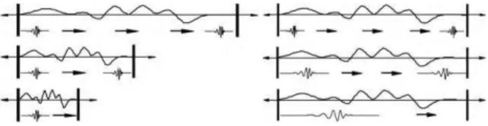
developed, namely non-decimated or Undecimated Wavelet Transform (UDWT). The UDWT requires more storage space than DWT and is computationally intensive, but is shift invariant, has no aliasing and provides more precise information for the frequency localization. The principles of conventional (decimated) DWT and undecimated DWT are compared, for the 1D case and for three levels, in Figure 2. By DWT the signal is downsampled by two, in contrast to UDWT, where the signal is left unchanged and filters are upsampled by two on each consecutive level (Fugal, 2009). UDWT has been shown to perform better at image denoising (Gyaourova, 2002).
Figure 2. Downsampling the signal in case of DWT (left) and upsampling the wavelet in case of UDWT (right) (Fugal, 2009).
Different UDWT algorithms have been developed that differ in decomposition and/or reconstruction method, but are all shift invariant. To mention the most important and frequently used algorithms: algorithm `a trous (Holschneider et al., 1990), Beylkin’s algorithm (Beylkin, 1992), undecimated WT (Mallat, 1991), stationary WT (Nason and Silverman, 1995) and Cycle-Spinning (Coifman and Donoho, 1995). The last algorithm is implemented in Matlab, where it is called the ε-decimated DWT and denoted by SWT. It averages some slightly different DWTs to define stationary wavelet transform.
2.2 Thresholding procedure
2.2.1 Thresholding method. Success of DWT denoising, this is to reduce noise while preserving details of the original surface, depends on the threshold limit. Different threshold methods have been proposed sharing a common approach, which is, to estimate the standard deviation of noise and multiply it by a certain value. The threshold can be applied globally or locally. In the global case one single value is applied to all detail coefficients and in the local case a different threshold value is chosen for each wavelet level. The thresholding method is selected based on data characteristics and overall noise distribution. In this research two thresholding methods are compared, namely the fixed form and the penalized.
If the signal-to-noise ratio is small, the fixed-form (universal) threshold proposed by Donoho and Johnstone (1994) is used. For 2D space, the fixed-form threshold TF is defined as:
��= � ∗ √ ∗ � � ∗ � (1)
Where σ is the noise standard deviation and [r,c] is the surface grid size. If the noise level is not known a-priori, σ is computed as the Median Absolute Deviation (MAD) of detail coefficients at the first decomposition level (global threshold) or at each decomposition level (local threshold).
A variant of the fixed form strategy of the wavelet shrinkage is the penalized thresholding method based on denoising results by Birgé and Massart (1997). The penalized threshold TP is defined as:
��= |� �∗ | (2)
Where t* is the penalty function to be minimized and equals:
�∗= �� � [− ∑ �2 , < + ��2(� + � ⁄ )]�
� = , … ,
(3)
Where α is the sparsity parameter, coefficients c(k) are sorted in decreasing order of their absolute value, and σ2 is the noise variance computed as explained above (for fixed-form). Three intervals for the sparsity parameter are proposed, namely penalized low 0 < α <1.5, penalized medium 1.5 < α <2.5 and penalized high 2.5 < α <10.
2.2.2 Thresholding mode. The selected threshold can be applied to a surface in either a soft or hard thresholding mode. For a case of surface profile, the principles as well as effects of thresholding modes are shown in Figure 3. In the hard mode, coefficients (black solid line) that are in absolute value lower than a threshold value (black dashed lines) are simply set to zero. In the soft mode, additional coefficients that are above the threshold value are reduced for the threshold value. Therefore, soft thresholding results in a smoother profile (blue dotted line) and hard thresholding introduces profile discontinuities (red dashed line). Hard thresholding provides an improved signal to noise ratio (Shim et al., 2001). In terms of image denoising, the soft thresholding is preferred, because it makes algorithms mathematically more tractable and avoids artificial and false structures (Donoho, 1995).
Figure 3. The principle of soft and hard thresholding.
3. ROUGHNESS PARAMETER
The roughness parameter introduced by Grasselli (2001) is based on the angular threshold concept and was initially developed to identify potential contact areas during direct shear testing of artificial rock joint. Highly accurate and detailed ATOS (Advanced TOpometric Sensor) measurements were used to reconstruct (triangulate) the surface of the rock joint. Based on joint surface damage patterns, it was found that only those areas of the joint surface that face the shear direction and are steeper than a threshold inclination θ∗ provide shear resistance. The sum of triangulated areas that are steeper than θ∗ (denoted as Aθ∗ and referred to as the total potential contact area ratio) is plotted against θ∗ (Figure 4).
Figure 4. Cumulative distribution of potential contact area ratio
Aθ∗ having a minimum inclination θ∗[ᵒ], which is computed with respect to average joint plane and analysis direction
(Grasselli, 2001).
Based on curve fitting and regression analysis, Grasselli proposed an empirical equation to express potential contact area ratio Aθ∗ as a function of θ∗:
Aθ∗= Ao∗ θmax∗ − θ∗⁄θmax∗ C (4)
Where Ao is the maximum possible contact area in the shear direction (when θ∗=0°), which is usually around 50% of the total surface area for fresh mated joint, θmax∗ is the maximum apparent dip angle of the surface in the shear (analysis) direction and θ∗ is the threshold inclination, this is the minimum apparent dip angle for applied normal load σn.
C is an empirical fitting parameter calculated via a non-linear least-squares regression that characterizes the shape of the cumulative distribution. Surface parameters Aθ∗, C and θmax∗ depend on the specific shear direction and 3D surface representation. A higher proportion of steeply inclined triangulated areas is indicative of a rougher surface, and is reflected by a larger area under the curve given by Eq. 4. This area, assuming Ao is 0.5, is taken as the roughness parameter R (Tatone and Grasselli, 2012) and is computed by:
R = θmax∗ ⁄ C + (5)
4. EXPERIMENTS AND RESULTS
Experiments were executed on ATOS measurements which have much higher precision than any TLS data. Therefore ATOS data are taken as a reference noise-free input data into performance analyses of denoising methods. The objective of this noise-controlled test is to make solid and firm guidelines for denoising TLS data acquired by Riegl VZ400 laser scanner (Riegl, 2015).
In the following section a detailed description of experimental workflow is followed by presentation of results, including the threshold values, the method noise, and the method sensitivity to noise.
4.1 Experimental workflow
Input data for experiments were acquired with highly accurate ATOS I measurement system (Capture3D, 2013). A rock joint formed in fossiliferous limestone having dimensions of 20×30 cm was imaged in the laboratory at approximately 0.5 m distance. On average, point density was 15 points per square millimetre. Further processing was performed in Matlab. First, the acquired dense point cloud was linearly interpolated into 1 mm grid, hereafter referred to original ATOS data (see Figure 9, top). Z-direction corresponds to roughness amplitude.
All together 12 wavelet denoising procedures were tested, which are a combination of:
Two 2D wavelet transform methods: DWT and SWT. Three thresholding methods: form global,
fixed-form local and penalised low.
Two thresholding modes: soft and hard.
DWT and SWT transforms were executed on four levels using a general purpose Daubechies wavelet db3 that has three vanishing moments and the filter length of 6 points. Reasons for the choice are given already in Section 2.
Threshold values are computed with equations given in Paragraph 2.2.1. Sigma for fixed-form global threshold equals the known standard deviation of added noise (values are written
in the following paragraph). Standard deviation for fixed-form local threshold is re-computed for each decomposition level as MAD of detail coefficients of the level. Penalised low threshold is a global value computed by sigma equal to MAD of detail coefficients of the first level and alpha of 1.5. The three threshold values are applied on detail coefficients in the two modes: soft and hard. Six different threshold combinations are denoted on the following figures as given in Table 1.
Denotation Threshold combination FGS Fixed-form Global threshold, Soft mode FGH Fixed-form Global threshold, Hard mode FLS Fixed-form Local threshold, Soft mode FLH Fixed-form Local threshold, Hard mode PLGS Penalised Low Global threshold, Soft mode PLGH Penalised Low Global threshold, Hard mode
Table 1. Denotation of threshold values and modes used in the following figures.
Two analyses were performed in order to justify suitability of the wavelet denoising methods for rock joint roughness estimation. First, the noise of a denoising method itself is analysed (method noise analysis) by applying denoising methods on original ATOS data. If assuming that ATOS data have no or very little noise and that a denoising method removes just noise and not also details, the output (denoised) surface should match the input surface. Second, original ATOS data is corrupted with different levels of Gaussian white noise and the method sensitivity to noise is studied as the noise increases. The aim of this controlled noise level experiment is to study dependence of thresholds and denoising method performance on amount of noise. Noise levels were chosen based on empirical noise estimation for the Riegl VZ400 laser scanner in (Vezočnik, 2011). His experiment showed that noise on concrete surfaces reaches maximum 2.2 mm for scanning distances up to 65 m and incidence angles up to 60ᵒ. Therefore in our experiment five noise levels were chosen, namely 0.5, 1, 1.5, 2 and 2.5 mm. Noise was added to grid points of original ATOS data and those noisy surfaces entered the denoising procedure. As an example, surface of 2 mm added-noise is shown in Figure 9, middle.
The Grasselli parameter was computed for the 12 denoised surfaces and original surface, as explained above. The analysis direction changes clockwise from 0ᵒ (+Y-axis direction) to 355ᵒ in 5ᵒ steps.
A comparative study of denoised surfaces and the original surface is based on three performance measures: (1) qualitative visual check of denoised surfaces, (2) height differences ΔZ and (3) differences of roughness parameters ΔR. Height differences ΔZ are computed as Δ = � − ��� �for each grid
point and roughness differences as Δ� = � � − � ��� � for each analysis (shear) direction.
4.2 Threshold values
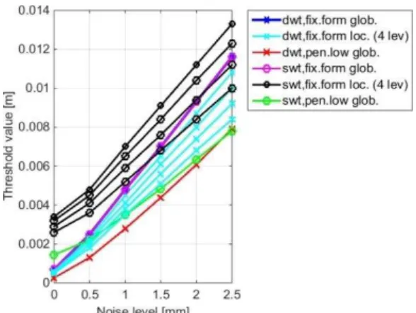
Threshold values computed for decomposed original (0 mm noise) and decomposed noisy (0.5 – 2.5 mm noise) surfaces are shown in Figure 5. All values linearly increase with noise level. Fixed-form local thresholds for DWT and SWT are presented by four lines – one for each decomposition level. Lines are following each other with the level number; from the upper line (higher threshold) of first level to the lower line (smaller threshold) of fourth level. Thus, threshold value decreases with decomposition level. Fixed-form global threshold values are, by
definition of our computation, the same for DWT and SWT. The other two SWT thresholds (fixed-form local and penalised low) are compared to corresponding DWT’s thresholds higher and increase slower with the noise.
Figure 5. Fixed-form global and local, and penalised low global threshold values for the DWT and SWT decomposition.
4.3 Method noise
Method noise analysis is performed on the original ATOS surface. Figure 6 shows mean and standard deviation of the two performance measures, ΔZ (left plot) and ΔR (right plot), versus denoising methods. Mean of ΔZ is as expected zero for all denoising methods, however the standard deviation, which indicates noise produced by denoising method, ranges from approximately 0.1 mm for DWT penalised low hard thresholding (left plot, red mark at PLGH) to 0.6 mm for SWT fixed-form local soft thresholding (left plot, blue mark at FLS). Similar pattern can be observed in error plot of ΔR, where the DWT penalised low hard thresholding surface shows the smallest mean roughness difference -0.3ᵒ (right plot, red mark at PLHG) compared to biggest mean difference of -9ᵒ by SWT fixed-form local soft thresholding (right plot, blue mark at FLS). In general, considering the wavelet transform and thresholding mode, method noise is lower in case of DWT and hard thresholding.
Figure 6. Error plot of ΔZ (left) and ΔR (right) for 12 denoising methods.
4.4 Method sensitivity to noise
Adding the five levels of noise to ATOS grid, the height differences ΔZ and roughness parameter differences ΔR were computed. Mean ΔZ is very close to zero for all 12 denoised surfaces (as seen already in Figure 6). Standard deviation �Δ , which shows how much noise is left in denoised surface, increases with the noise level and is bigger in case of soft thresholding for both, DWT and SWT transforms (see Figure 7). Figure 7 shows that the noise is greatly reduced, except in case of 0.5 mm noise level, when fixed form global and local soft threshold were applied for DWT (left plot, blue and red
line) and all three soft thresholds for SWT (right plot, red, blue and black line).
Figure 7. Standard deviation �Δ versus noise levels for DWT (left) and SWT (right) denoised surfaces applying six
thresholds.
Figure 8 shows distribution of roughness parameter differences ΔR versus noise level. Mean ΔR decreases (i.e. roughness estimation error ΔR increases), whereas the standard deviation of ΔR does not show clear trend. Surfaces contaminated with higher level of noise become smoother after wavelet denoising. Decrease of roughness with increase of noise can be explained with higher threshold values (Figure 5), which filter more surface details. An exception is SWT penalised low hard method, which does not show a clear trend.
Figure 8. Error plot of ΔR versus noise levels for DWT (left) and SWT (right) denoised surfaces applying six thresholds.
Comparing DWT and SWT results for the common fixed-form global threshold (in Figure 8 – blue and turquoise line for soft and hard thresholding mode, respectively), SWT denoising results in much underestimated roughness.
Hard thresholding performs better than soft thresholding since standard deviation of ΔZ is lower and absolute values of ΔR are smaller. However, the visual check of denoised surfaces shows that hard thresholding especially in combination with conservative penalised-low thresholding results in a number of spikes (see Figure 9, bottom). Spikes are left overs of unfiltered noise. Spikes appear in DWT and SWT denoised surfaces, and become higher with increasing noise level, as shown especially for penalised low hard thresholding.
5. DISCUSSION AND CONCLUSIONS
Experiments on the simulated noisy ATOS data show positive results: by applying a wavelet-based denoising procedure noise is successfully reduced and roughness estimates are much closer to the reference values. All investigated denoising methods significantly reduce standard deviation of height differences. Denoised surfaces contain less than 1 mm noise. Roughness is on average (for different noise levels and denoising methods) underestimated, which means that in addition to noise, some surface details are also removed.
Figure 9. Visual comparison of 1 mm grid surfaces: original ATOS (top), noisy surface with 2 mm added noise (middle) and
same surface denoised by DWT, penalised low hard thresholding (bottom).
5.1 Concluding remarks
DWT versus SWT: For the investigated thresholding procedures and for the five noise levels, DWT provides better results considering our application; this is for reliable rock joint roughness estimation. SWT smoothens surfaces more than DWT. The first reason is the underlying computation of SWT, which averages many different DWTs. Secondly, the same thresholding methods (fixed-form local and penalised low) result in higher SWT thresholds. DWT is preferable also because MAD of first level DWT detail coefficients equals the standard deviation of noise.
Fixed-form versus penalised threshold: It is known that the penalised threshold is more conservative than fixed-form. This means that the penalised threshold retains more coefficients and the fixed form threshold removes noise more efficiently. In our experiments the penalised low threshold results in noise spikes in denoised surfaces (as reported also in Coifman and Donoho, 1995), and the fixed-form filters out surface details and returns lower roughness values.
Soft versus hard mode: Soft thresholding, compared to hard thresholding, smoothens the surface, since unfiltered coefficients are reduced for the threshold. This phenomena appears unfavourable for rock surface roughness estimation. On
the other hand, soft thresholded surfaces look smoother and more natural (without artificial spikes).
Local versus global threshold: Local thresholds decrease with level, which agrees with the assumption that higher levels of lower resolution contain less noise. On the contrary, global thresholds computed from first level detail coefficients remains constant and therefore removes more actual details on higher levels. This is indicated by results of DWT denoising, where fixed-form local thresholds provide more realistic roughness estimation than the fixed-form global threshold.
In conclusion, the suggested denoising method is DWT penalised low hard local thresholding. Having smaller mean and standard deviation of roughness differences is preferred over visually smoother surface.
5.2 Outlook
Results of this research show that inherent TLS range noise can potentially be removed by post- processing using wavelet based denoising. However, further research is needed to support the proposed method for arbitrary scanning geometry and rock joint characteristics.
In our experiment we assumed that the rock surface is scanned in the perpendicular direction; thus z-direction (in which denoising is performed) corresponds to range measurement direction. In the case of non-perpendicular acquisition, denoising in polar coordinates space (range image) would be needed.
Beside wavelet transform, other image denoising methods exist, for example Non-Local Mean(Buades et al., 2005). A short trial showed promising results. However, an elaborated investigation is needed to find the optimum input parameters (patch and search window size) for rock surface roughness estimation.
ACKNOWLEDGEMENTS
The Slovenian National Building Institute and Civil Engineering Institute enabled data acquisition with ATOS measuring system. Klemen Kregar from University of Ljubljana processed TLS reference targets’ centres with his image matching algorithm.
REFERENCES
Barton, N., Choubey, V., 1977. The Shear Strength of Rock Joints in Theory and Practice. Rock Mechanics and Rock Engineering, vol. 10, pp. 1-45.
Barton, N., 1973. Review of a New Shear-Strength Criterion for Rock Joints. Engineering Geology, vol. 7, pp. 287-332.
Beylkin, G., 1992. On the Representation of Operators in Bases of Compactly Supported Wavelets. SIAM Journal on Numerical Analysis, 29 (6), pp. 1716–40.
Birgé, L., Pascal, M., 1997. From Model Selection to Adaptive Estimation. In Festschrift for Lucien Le Cam. Pollard, D., Torgersen, E., Yang, G. L. (eds.), pp. 55–87. Springer New York.
Bitenc, M., Kieffer, D. S., Khoshelham, K., Vezočnik, R., 2015. Quantification of Rock Joint Roughness Using Terrestrial Laser Scanning. In Engineering Geology for Society and Territory -
Volume 6. Lollino, G., Giordan, D., Thuro, K., Carranza-Torres, C., Wu, F., Marinos, P., Delgado, C. (eds.), pp. 835–38. Springer International Publishing.
Buades, A., Coll, B., Morel, J., 2005. A Non-Local Algorithm for Image Denoising. In IEEE Computer Society Conference on Computer Vision and Pattern Recognition, vol. 2, pp.60–65.
Capture3D, 2013. Atos I, Configurations. http://www.capture3d.com/products-ATOSI-configuration.html.
Coifman, R. R., Donoho, D. L., 1995. Translation-Invariant de-Noising. Springer New York.
Daubechies, I., 1992. Ten Lectures on Wavelets. CBMS-NSF Regional Conference Series in Applied Mathematics. Society for Industrial and Applied Mathematics.
Donoho, D. L., Johnstone, J. M., 1994. Ideal Spatial Adaptation by Wavelet Shrinkage. Biometrika, vol. 81 (3), pp. 425–55.
Donoho, D. L., 1995. De-Noising by Soft-Thresholding. Information Theory, IEEE Transactions on Information Theory, vol. 41 (3), pp. 613–27.
Fardin, N., Stephansson, O., Feng, Q., 2004. Application of a New in Situ 3D Laser Scanner to Study the Scale Effect on the Rock Joint Surface Roughness. International Journal of Rock Mechanics and Mining Sciences, vol. 41 (2), pp. 329–35.
Fernández-Steeger, T., Wiatr, T., Azzam, R., 2009. Terrestrial Laser Scanning in Engineering Geology. In 17. Tagung Für Ingenieurgeologie Und Forum „Junge Ingenieurgeologen.
Fowler, A., France, J. I., Truong, M., 2011. Applications of Advanced Laser Scanning Technology in Geology. Riegl USA.
Fugal, D. L., 2009. Conceptual Wavelets in Digital Signal Processing. San Diego, Calif: Space & Signals Technical Publishing.
Grasselli, G., 2001. Shear Strength of Rock Joints Based on Quantified Surface Description. PhD thesis. Lausanne, EPFL.
Gyaourova, A., Chandrika, K., Imola K. F., 2002. Undecimated Wavelet Transforms for Image de-Noising. Report, Lawrence Livermore National Lab., CA 18.
Heckbert, P. S., 1989. Fundamentals of Texture Mapping and Image Warping.
Holschneider, M., Kronland-Martinet, R., Morlet, J., Tchamitchian, P., 1990. A Real-Time Algorithm for Signal Analysis with the Help of the Wavelet Transform. In Wavelets. Inverse Problems and Theoretical Imaging. Combes, J.-M., Grossmann, A., Tchamitchian, P. (eds,), pp. 286–97. Springer Berlin Heidelberg.
ISRM, 1978. Suggested Methods for the Quantitative Description of Discontinuities in Rock Masses. International
Journal of Rock Mechanics, Mining Sciences and
Geomechanics Abstracts, vol. 15, pp. 319–68.
Khoshelham, K., Altundag, D., Ngan-Tillard, D., Menenti, M., 2011. Influence of Range Measurement Noise on Roughness Characterization of Rock Surfaces Using Terrestrial Laser
Scanning. International Journal of Rock Mechanics and Mining Sciences, vol. 48 (8), pp. 1215–23.
Lichti, D. D., 2007. Error Modelling, Calibration and Analysis of an AM–CW Terrestrial Laser Scanner System. ISPRS Journal of Photogrammetry and Remote Sensing, vol. 61 (5), pp. 307–24.
Lichti, D. D., Jamtsho, S., 2006. Angular Resolution of Terrestrial Laser Scanners. The Photogrammetric Record, vol. 21 (114), pp. 141–60.
Mallat, S., 1991. Zero-Crossings of a Wavelet Transform. Information Theory, IEEE Transactions on Information Theory, vol. 37 (4), pp. 1019–33.
Nason, G. P., Silverman, B. W., 1995. The Stationary Wavelet Transform and Some Statistical Applications. In Wavelets and Statistics, vol. 103, pp. 281–300. Springer-Verlag.
Patton, F. D., 1966. Multiple Modes of Shear Failure in Rock. Presented at the 1st ISRM Congress. International Society for Rock Mechanics.
Pesci, A., Teza, G., Bonali, E., 2011. Terrestrial Laser Scanner Resolution: Numerical Simulations and Experiments on Spatial Sampling Optimization. Remote Sensing,vol. 3 (1), pp. 167–84.
Priest, S. D., 1993. Discontinuity Analysis for Rock Engineering. Springer.
Rasouli, V., Harrison, J. P., 2004. A Comparison of Linear Profiling and an in-Plane Method for the Analysis of Rock Surface Geometry. International Journal of Rock Mechanics and Mining Sciences, vol. 41, Supplement 1 (0), pp. 133–38.
Riegl, 2015. Laser Scanner VZ-400, Datasheet. (April, 20015)
http://www.riegl.com/nc/products/terrestrial-scanning/produktdetail/product/scanner/5/.
Shim, I., Soraghan, J. J., Siew, W. H., 2001. Detection of PD Utilizing Digital Signal Processing Methods. Part 3: Open-Loop Noise Reduction. Electrical Insulation Magazine, IEEE 17 (1), pp. 6–13.
Siefko, S., 2010. Automated Rock Mass Characterisation Using 3D Terrestrial Laser Scanning. PhD thesis. International Institute for Geo-information Science and Earth Observation, Enchede, The Netherlands.
Smigiel, E., Alby, E., Grussenmeyer, P., 2008. Terrestrial Laser Scanner Data Denoising by Range Image Processing for Small-Sized Objects. The International Archives of the Photogrammetry, Remote Sensing and Spatial Information Sciences, vol. 37.
Smigiel, E., Alby, E., Grussenmeyer, P., 2011. TLS Data Denoising by Range Image Processing. The Photogrammetric Record, vol. 26 (134), pp. 171–89.
Soudarissanane, S., Lindenbergh, R., Menenti, M., Teunissen, P., 2011. Scanning Geometry: Influencing Factor on the Quality of Terrestrial Laser Scanning Points. ISPRS Journal of Photogrammetry and Remote Sensing, vol. 66 (4), pp. 389–99.
Sturzenegger, M., Stead, D., 2009. Close-Range Terrestrial Digital Photogrammetry and Terrestrial Laser Scanning for
Discontinuity Characterization on Rock Cuts. Engineering Geology, vol. 106 (3–4), pp. 163–82.
Tatone, B., Grasselli, G., 2012. An Investigation of Discontinuity Roughness Scale Dependency Using High-Resolution Surface Measurements. Rock Mechanics and Rock Engineering, vol. 46 (4), pp. 657-681.
Tonon, F., Kottenstette, J. T., 2006. Laser and Photogrammetric Methods for Rock Face Characteization. Report on a Workshop Held June 17-18, 2006 in Golden, Colorado. American Rock Mechanics Association.
Vezočnik, R., 2011. Analysis of Terrestrial Laser Scanning Technology for Structural Deformation Monitoring. PhD thesis. University of Ljubljana, Ljubljana, Slovenia.
Zhang, Y., Liu, J., Li, M., Guo, Z., 2014. Joint Image Denoising Using Adaptive Principal Component Analysis and Self-Similarity. Information Sciences, vol. 259 (0), pp. 128–41.

![Figure 4. Cumulative distribution of potential contact area ratio A θ ∗ having a minimum inclination θ ∗ [ᵒ] , which is computed](https://thumb-eu.123doks.com/thumbv2/123dok_br/18395915.358108/4.892.153.371.941.1076/figure-cumulative-distribution-potential-contact-minimum-inclination-computed.webp)