A DISCRETE WAVELET TRANSFORM – SINGULAR VALUE DECOMPOSITION SYSTEM FOR IMAGE CODING

(1)

121

Journal of Applied Research and Technology

A

DISCRETE WAVELET TRANSFORM – SINGULAR VALUE

DECOMPOSITION SYSTEM FOR IMAGE CODING

H. de Jesús Ochoa-Domínguez, K. R. Rao

ABSTRACT

A system that combines techniques of wavelet transform (DWT) and singular value decomposition (SVD) to encode images is presented. The image is divided into tiles or blocks of 64x64 pixels. The decision criterion as to which transform to use is based on the standard deviation of the 8x8 pixel subblocks of the tile to encode. A successive approximation quantizer is used to encode the subbands and vector quantization/scalar quantization is used to encode the SVD eigenvectors/eigenvalues, respectively. For coding color images, the RGB components are transformed into YCbCr before encoding in 4:2:0 format. Results show that the proposed system outperforms the JPEG and approaches the JPEG2000.

RESUMEN

Se presenta un nuevo sistema que combina técnicas de transformada wavelet (DWT) y descomposición en valores singulares (SVD) para codificar imágenes. Las imágenes se dividen en cuadros de 64x64 pixeles. Para decidir qué transformada utilizar, se utiliza un criterio basado en la desviación estándar de subbloques de 8x8 pixeles del bloque a codificar. Las subbandas, resultadas de aplicar la DWT, se codifican utilizando un cuantizador de aproximaciones sucesivas. Los eigenvectores y eigenvalores, resultados de la aplicación SVD, se codifican utilizando cuantización vectorial y escalar, respectivamente. Antes de codificar imágenes a color, las componentes RGB se transforman a YCbCr en formato 4:2:0. Los resultados muestran que con el sistema propuesto se logra mucho mayor compresión que JPEG y se aproxima bastante al nuevo estándar de compresión JPEG2000.

KEYWORDS:Wavelet Transform, Singular Value Decomposition, HC-RIOT, SPIHT, Scalar Quantization, Vector Quantization, Image Coding, HDCTSVD.

1. INTRODUCTION

A hybrid DCT-SVD (HDCTSVD) image coding algorithm was developed earlier by Dapena and Ahalt [1]. They showed that the hybrid technique performs well on low spatially correlated images. In this paper, another hybrid approach called HDWTSVD is proposed. This method takes advantage of the multi resolution – multi frequency capabilities of the discrete wavelet transform (DWT). Various adaptive features such as selection of the DWT or singular value decomposition (SVD), discarding low magnitude eigenvalues and corresponding eigenvectors, VQ and/or SQ of eigenvectors

(2)

122 Vol. 5 No. 2 August 2007

downsampled chrominances is one less than the corresponding luminance component for each color tile. Using standard test images, the performance of the HDWTSVD is compared with that of the HDCTSVD, JPEG and JPEG2000 [5], [6]. Details of the proposed algorithm are described below.

2. SELECTION OF DWT OR SVD

The decision criterion as to which transform to use is based on two simple parameters: the average standard deviation (ASTD) of 8x8 subblocks of the (64x64) size tile to encode, which is nothing but the standard deviation of 8x8 subblocks of a tile averaged over all subblocks of the tile; and the standard deviation of the standard deviations (SSTD) of the same 8x8 subblocks of a tile. The subblock size of (8x8) pixels is selected after an evaluation of various subblock sizes, including the (64x64) tile. The selection of the DWT or SVD, for color tiles, is based on the ASTD and SSTD of the luminance tile only.

3.

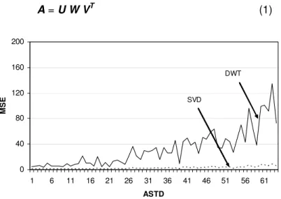
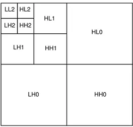
INITIAL TESTS

This test consists of considering the high frequencies or low correlated areas of tiles of different monochrome images to compare the SVD and the DWT. Figure 1 shows the plot of the ASTD vs. the mean squared error (MSE) of the encoded tiles using the DWT and the SVD. The encoding process consisted of decomposing each tile into 3 levels of wavelet decomposition (see Fig. 2). The high-high subband of the first level or level zero (HH0) was discarded (all the coefficients are set to zero). The HH0 subband consists of 32x32 coefficients, which means that one quarter of the total number of coefficients were discarded. The tiles were recovered by applying inverse DWT and the MSE was calculated. Then, each original tile was subdivided into subblocks (A_{) of 8x8 pixels and the SVD was applied. Assuming}

block A was full rank (r), each subblock was decomposed into two (8x8) orthogonal matrices containing the eigenvectors (U_andVT_{) and one (8x8) diagonal matrix containing the eigenvalues (}W_{) as follows [2],}

[7]:

A = U W VT (1)

0 40 80 120 160 200

1 6 11 16 21 26 31 36 41 46 51 56 61

ASTD

MSE

SVD

DWT

(3)

123

After rearranging the eigenvalues in decreasing order, the seventh and eighth eigenvalues were discarded. This means that one quarter of the total number of eigenvalues of a tile (64 subblocks) were discarded, followed by inverse SVD (ISVD). Figure 1 shows that the MSE increases as the ASTD does, which means that the DWT introduces more error for tiles with high ASTD.

Figure 2. Three levels of wavelet decomposition

The filter bank used to implement the DWT was the Daubechies 9/7 [8], factored into lifting steps to help reduce computational complexity [9]. Symmetric periodic extension was used on each tile compressed using the DWT, to help reduce the block artifacts of the reconstructed tile and the coefficient expansion at the output of the analysis bank [10].

The DWT and the SVD are computationally expensive, but the SVD is even more expensive because the computation of the basis vectors is time-consuming [2], [7]. This imposes the following restrictions on the HDWTSVD system.

1. There are tiles that exhibit low and high pixel activities. Low pixel activities are low-ASTD tiles and high pixel activities are high-ASTD tiles.

2. Tiles with low pixel activity are usually low-frequency blocks with high correlation.

3. Tiles with high pixel activity contain edges, high frequencies, edges and high frequencies, or edges and low frequencies (these can be sharp edges).

4. Edges are high-frequency regions which have more masking effects and require large codebooks to be encoded in order to reduce the distortion.

5. Combination of edges and high pixel activity tiles will increase the distortion in the recovered tiles but will be less noticeable visually .

5. Tiles with high pixel activity or combination of low pixel activity and smooth edges will be compressed using SVD.

7. The decision taken on whether to use DWT or SVD must be simple.

Restriction 7 imposes us to look for a fast decision. From Fig. 1, we can see that the ASTD could be a good indicator of the pixel activity. High pixel activity tiles result in high ASTD. It seems that from this figure we can select a threshold of ASTD, but that is false because the test set contains any type of tiles as mentioned in restriction 3. Sharp edges should not be encoded by using SVD because of restriction 4. A tile containing a sharp edge can produce high ASTD. Therefore, the ASTD of a sharp edge would be a wrong indication and may be understood by the system as a high pixel activity tile. However, if one calculates the standard deviation of the already calculated standard deviations (SSTD) of 8x8 subblocks, we see that the sharp edges result in SSTD much higher than low or high pixel activity tiles. The threshold for the ASTD can be calculated by taking the ASTD of tiles containing a combination of sharp

HH0

HH1

HH2 HL2

LH2 LL2

LH1

HL1

HL0

(4)

124 Vol. 5 No. 2 August 2007

edges and smooth areas. Tiles to calculate this threshold were taken from Baboon, Tiffany, Boat, and Elaine images in the database [11]. Table 1 shows the average standard deviation of tiles containing a combination of sharp edges and low pixel activity areas only. From this table, we can set a threshold of 20 for the ASTD.

ASTD

18.30 18.33 18.22 17.01 19.36 19.33 18.01 16.06 19.63 17.15 18.51 15.21 18.56 18.00 18.23 16.45 18.17 18.14 18.18 18.62 19.05

Average of ASTD 18.02

Variance of ASTD 1.21

Standard deviation of ASTD 1.10

Table 1. ASTD of tiles containing sharp edges and low pixel activity

The SSTD indicates how deviated the standard deviations of the mean are; if this value is very high then, as long as the ASTD is also high, we are dealing with a sharp edge,. The SSTD can be calculated after calculating the standard deviations of the 64 subblocks of a tile and the ASTD.

Table 2 shows the typical SSTD value for tiles containing sharp edges, low pixel activity, high pixel activity, and a combination of high and low pixel activity.

Table 2. SSTD of tiles containing (a) sharp edges, (b) low pixel activity, (c) high pixel activity, and (d) combination of high and low pixel activity

Pixel activity SSTD Sharp edge 23.01

(5)

125

Figure 3. Barbara image divided into tiles showing tiles 45 and 47

The selected threshold for SSTD is 12. Below this value, we include tiles with low and high pixel activity but not sharp edges. The images used to calculate this threshold are the same as the images used to find the ASTD [11].

Figure 3 shows the 512x512 Barbara image divided into tiles of 64x64 pixels. The image shows tiles 45 and 47; both of them are high ASTD tiles, but tile 47 contains an edge, which produces high distortion. Figure 4 shows the area of tiles which are good candidates to be compressed using SVD for this image. This is a selective area that contains tiles with an ASTD greater or equal to 20 and an SSTD less than or equal to 12. This area engulfs tiles 31, 33, 45, 48, and 54. Tile 47 has an ASTD of about 30 and an SSTD of about 16. With the ASTD as the only threshold, this tile was one of the candidates for SVD.

Figure 4. Candidate tiles for SVD of Barbara image

The HC-RIOT [4] is a modified SPIHT [3] that considers scalability, perceptual optimization, error resilience, and spatial segmentation strategies. The HC-RIOT takes advantage of the DWT to exploit multiresolution, self-similarity in subbands, and spatial localization properties. This approach is combined

4

0

5

10

15

20

25

30

35

40

2

4

6

8

10

12

14

16

18

20 S

S

T

D

33

48

45 54

31 47

Th_ASTD > = 20

Th_SSTD < = 12

(6)

126 Vol. 5 No. 2 August 2007

with a two-stage ZTE/SPIHT algorithm for entropy coding of the image that considers progressive transmission, scalability, and perceptual optimization. The bit stream is initially transmitted using three layers. A base layer with a fixed bit rate always gives a decodable image, an enhancement layer with progressive transmission containing critical bits necessary to keep the encoder and decoder synchronized in image reconstruction and enable picture quality improvements, and another enhancement layer that only contains information necessary to improve the image quality. The HC-RIOT encodes well the tiles with sharp edges.

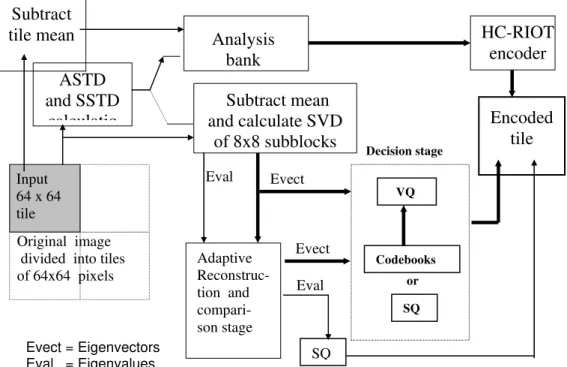
4. ENCODER

Figure 5 shows the diagram of the encoder. The input image is divided into blocks or tiles of 64x64 pixels. The tile size was decided based on the number of SVD subblocks per tile to calculate and the number of subband decomposition levels. That means that we selected a tile size, which could be well decorrelated by the DWT and the computational complexity of the SVD could not be exacerbated. The ASTD and the SSTD are calculated. If the ASTD of the tile is equal to or greater than 20, and the SSTD is equal to or less than 12, the tile is subdivided into subblocks of 8x8 pixels and then compressed independently by using SVD. First, the mean of the subblock is subtracted and encoded using 8 bits. Then, the SVD is applied to each subblock to calculate matrices U_,VT_andW_{. In the adaptive}

reconstruction and comparison stage, the eigenvalues are rearranged in decreasing order (from the highest to the lowest) and discarded progressively, by setting them to zero, from the lowest to the highest until an MSE for the subblock is met (after exhaustive tests the MSE set for this unit was 5). The total MSE of the subblock is calculated each time an eigenvalue is discarded by using equation (2).

∑

+ = σ

= r

1 q n

2 n

NxN 1

MSE (2)

where σn is the nth largest eigenvalue, NxN is the block size (8x8), r is the rank, and q is the number of

eigenvalues retained.

After meeting the MSE requirement for a subblock, the resulting eigenvalues are coded using uniform scalar quantizers of 8,8,7,7,6,6, and 4 bits, respectively; and their corresponding eigenvectors are sent to the decision stage. The eighth eigenvalues/eigenvectors are discarded. The adaptive reconstruction and comparison stage helps us to discard adaptively the eigenvalues and eigenvectors that do not introduce a significant visual error.

The decision stage consists of three uniform scalar quantizers of 7, 7 and 5 bits, respectively; and seven codebooks of lengths 256, 128, 32, 32, 32, 16, and 8. The scalar quantizers and the codebooks are the same for the eigenvectors of matrices U _andVT_{. After quantization of one eigenvector of matrix}U_{, the}

process is repeated for the eigenvector in matrix VT_.

(7)

127

Figure 5. The HDWTSVD encoger

In previous tests with low and high pixel activity images, it was observed that the first eigenvalue/eigenvector plays the most important role in reducing the subblock MSE. Therefore, the MSE allowed for this eigenvalue has to be very small as compared to the other thresholds. In preliminary tests, for high pixel activity tiles (high ASTD) taken from some textures and not containing sharp edges, the average number of eigenvectors/eigenvalues per tile was 6.82. The total number of tiles used was 128 taken from different images [11]. This means that the last two eigenvalues/eigenvectors are less probable to exert a noticeable effect in a subblock. This allows us to have a codebook of reduced size for the 7th eigenvector and to discard the 8th eigenvector. The codebooks sizes were determined after exhaustive tests. The LBG algorithm was used [12] to train the codebooks and the training images are taken from [11].

If the ASTD of the tile is less than 20 and/or the SSTD greater than 12, the tile is compressed using the Daubechies 9/7 filter bank factored into lifting steps. The tile mean is subtracted before filtering and quantized to 8 bits; then, the tile, or subband, is extended using symmetric periodic extension to help reduce the block artifacts effect in the reconstructed tile and to avoid coefficients expansion. Each 64x64 tile is decomposed into a maximum of three levels; level two or last decomposition level is an 8x8 block. The subband coefficients are non-integer; therefore, they are rounded to the nearest integer, which causes a minimal loss in PSNR. The resulting subbands, after three levels of decomposition, are encoded using the HC-RIOT [4].

ASTD

and SSTD

calculatio

Subtract

tile mean

Input 64 x 64 tile

Original image divided into tiles of 64x64 pixels

Analysis

bank

HC-RIOT

encoder

Subtract mean

and calculate SVD

of 8x8 subblocks

Adaptive Reconstruc- tion and comparison stage

Encoded

tile

Evect SQ Eval Eval VQ Codebooks SQ or Decision stage Evect

(8)

128 Vol. 5 No. 2 August 2007

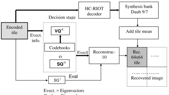
5. DECODER

Figure 6 shows the diagram of the decoder. The first bit of the encoded tile is read, and if the tile belongs to SVD, it is recovered in 8x8 subblocks. After reading the number of eigenvalues encoded for a specific subblock, another bit is read. This bit informs the decoder if the information for the first eigenvector belongs to an entry index (8 bits), or if the following 56 bits (7 bits x 8 eigenvectors’ components) are the quantized eigenvector’s component. The process is repeated to recover the first quantized eigenvector of the matrix VT_{and the second eigenvectors of}U_andVT_{. The third eigenvectors of}U_andVT _are

recovered in the same way except that if the information belongs to the component’s eigenvector, then the eigenvector will be retrieved in a packet of 40 bits (5 bits x 8 eigenvectors’ components). The 4th, 5th, 6th, and 7th eigenvectors of matrices U_andVT_{are retrieved by reading the indices of their}

respective codebooks. The eigenvalues are retrieved by reading and applying inverse quantization to the quantized values.

After applying inverse SQ/VQ, the eigenvalues and eigenvectors are decoded and an approximation of each subblock is recovered as Aˆ =U W VT. Then the process to recover another 8x8 subblock is repeated until the tile is reconstructed

.

Figure 6. The HDWTSVD decoder

6. CODING OF COLOR IMAGES

The HDWTSVD system to encode color images is shown in Figure 7. The input image has 512 x 512 8-bit-PCM RGB components. These components are transformed into YCbCr format, and the chrominance components (Cb, Cr) are downsampled by a factor of 2 before encoding. The luminance component is divided into tiles of 64x64 samples and the chrominances into tiles of 32x32 samples. Each tile contains one luminance component (Y) and two chrominance components with one quarter the resolution of the luminance component. The choice between DWT or SVD depends on the ASTD and SSTD of the Y component. If the tile is inside the area shown in Figure 4, the Y component and the downsampled Cb

Encoded tile

HC-RIOT decoder

Synthesis bank Daub 9/7

Reconstruc-

10

…..

….. ……….

Recovered image Rec.

64x64 tile Add tile mean

SQ-1

VQ-1

Codebooks

SQ-1

o

Decision stage

Evect. info.

Eval

Evect

(9)

129

and Cr are encoded using SVD; otherwise, DWT is used. If DWT is used, three levels of subband decomposition to Y and two levels of subband decomposition to Cb and Cr are applied.

Figure 7. The HDWTSVD system for color images

After decoding each component and each tile, the resulting Cb and Cr are upsam-pled by a factor of 2 both horizontally and vertically; color transformed to RGB, and each color component clipped in the interval from 0 to 255.

7. RESULTS

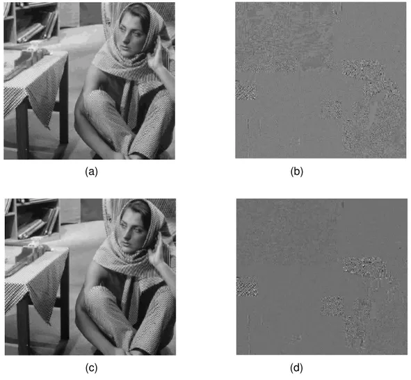
Figure 8 shows the Barbara image compressed at (a) 0.5 bpp with PSNR of 30.30 dB, and (c) 1.05 bpp with PSNR of 35.26 dB. The error images are shown in Figure 7 (b) and (d), respectively.

Y R

B

G

Color transfor-

mation.

Cb

HDWTSVD (Encoder)

Cr

HDWTSVD (Decoder) Input

image

R

B

G

Recons-tructed image

Downsampling Cb,Cr and tiling Y,Cb,Cr

64x64

32x32 32x32

Upsampling Cb, Cr Cr

Cb

Y Color

transfor- mation.

Cr(32x32) Cb(32x32) Y (64x64)

(10)

130 Vol. 5 No. 2 August 2007

(a) (b)

(c) (d)

Figure 8. Barbara image compressed at (a) 0.5 bpp, PSNR = 30.30 dB, (b) the error image, and (c) 1.05 bpp PSNR = 35.26, (d) the error image

We can see from the error images of 8 (b) and 8 (d), that the smooth areas compressed using DWT are changing. From low bit rate (0.5 bpp) we can see more perceptual error than for high bit rate (1.05 bpp). The areas compressed by SVD (corner of the table and some parts of the pants of Barbara) show a constant error because the encoding scheme is fixed and calculated to give the best quality of a tile for low bit rates.

(11)

131

0.2 0.4 0.6 0.8 1 1.2 1.4 1.6 1.8 2

20 24 28 32 36 40 44

Bit rate (bpp) PSNR (dB)

HDCTSVD threshold coding HDWTSVD

.

JPEG baseline JPEG2000

Figure 9. Comparison of the HDWTSVD with JPEG2000, JPEG baseline, and HDCTSVD using threshold coding for the Barbara image

Figure 10 shows the color Lena image compressed at (a) 0.5 bpp with PSNR of 33.68 dB and (b) error image of the R component, (c) error image of the G component and (d) error image of the B component.

(a) (b)

(c) (d)

(12)

132 Vol. 5 No. 2 August 2007

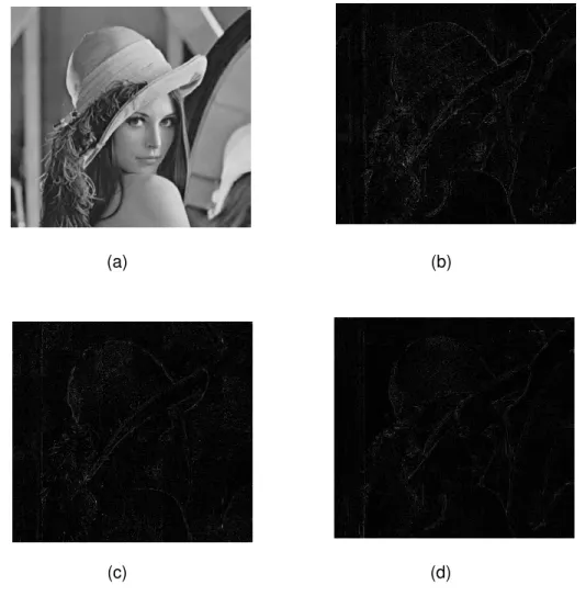
Figure 11 shows the color Lena image compressed at (a) 0.99 bpp with PSNR of 36.01 dB. and (b) error image of the R component; (c) error image of the G component, and (d) error image of the B component.

(a) (b)

(c) (d)

Figure 11. (a) Lena image at 0.99 bpp and PSNR of 36.01 dB, (b) error image of the R component, (c) error image of the G component, and (d) error image of the B component

(13)

133

0 0.5 1 1.5

26 28 30 32 34 36 38 40 42

JPEG2000 Color HDWTSVD

JPEG baseline

Bitrate (bpp) PSNR (dB)

Figure 12. Comparison of the HDWTSVD with JPEG2000 and JPEG baseline for the Lena image

8. CONCLUSIONS

In this research, a new system that combines techniques of DWT and SVD has been presented. Previous results to this work were published in [13], [14]. In this research, better quality images for both low and high bit rates have been obtained by optimizing each stage of the hybrid system. The advantage of the proposed system is that by tiling an image, one can take advantage of the local correlation. The decision on what transform to use is fast and based on the simple criterion of the ASTD and the SSTD only. The introduction of the adaptive reconstruction stage helps us to save bits in tiles compressed using SVD by reducing the number of eigenvectors and eigenvalues encoded. The decision stage helps us to increase the image quality adaptively. The periodic symmetric extension of the tiles is simple and helps to remove the block artifacts of the reconstructed images. No filter to reduce block artifacts, at low bit rates, was used as in JPEG or JPEG2000. Tiles are small and codebook sizes are short. Therefore, the algorithm can be well implemented in small memory systems. The encoding of the eigenvectors and the eigenvalues is simple.

Results show that the recovered images are of very good quality and Figs. 8 and 11 show that the system outperforms the HDCTSVD and JPEG baseline and approaches JPEG2000.

(14)

134 Vol. 5 No. 2 August 2007

9. REFERENCES

[1] Dapena and S. Ahalt, “A hybrid DCT-SVD image-coding algorithm,” IEEE Trans. CSVT, vol. 12, pp.114-121, Feb. 2002

[2] H. C. Andrews, Computer Techniques in Images Processing. NY and London: Academic Press, 1970.

[3] A. Said and W.A. Pearlman, “A new fast and efficient coder based on set partitioning in hierarchical trees,” IEEE Trans. CSVT, vol. 6, pp.243-250, June 1996.

[4] Y. F. Syed, A low bit rate wavelet-based image coder for transmission over hybrid networks. Doctoral Dissertation, University of Texas at Arlington, 1999.

[5] K.R. Rao and J.J. Hwang, Techniques and Standards for Image, Video and Audio Coding. Upper Saddle River, New Jersey: Prentice Hall, 1996.

[6] ISO/IEC FDIS 15444-1, JPEG 2000 Part I Final Draft International Standard, Aug. 2000.

[7] A.K. Jain, Fundamentals of Digital Image Processing. Englewood Cliffs, NJ: Prentice-Hall, 1989.

[8] A I. Daubechies, Ten Lectures on Wavelets. Rutgers University and AT&T Bell Laboratories, SIAM, 1992.

[9] I. Daubechies and W. Sweldens, “Factoring wavelet transforms into lifting steps,” J. Fourier Anal. Appl., vol. 4, pp. 247-269, 1998.

[10] M. Smith and S. Eddins, “Analysis/Synthesis techniques for subband image coding,” IEEE Trans. ASSP, vol. 38, pp. 1446-1456, Aug. 1990.

[11] http://sipi.usc.edu/services/database/

[12] Y. Linde, A. Buzo, and R. M. Gray, “An algorithm for vector quantizer design,” IEEE Trans. Communications, vol. 28, pp. 84-95, Jan. 1980.

[13] H. Ochoa and K.R. Rao, “A New HDWTSVD Coding System for Monochromatic Images,” WSEAS Transaction on Signal Processing, vol. 1, pp. 419-424, Dec. 2005.

(15)

135

Authors Biography

Humberto de Jesús Ochoa- Domínguez

Received the B.Sc. and M.Sc. degrees in electronic engineering from the Instituto Tecnológico de Toluca (ITT), in 1992 and 1998 respectively, and the Ph.D. degree in electrical engineering from the Institut National Polytechnique de Toulouse (INPT), France, in 2002.

In 1992 he joined the Instituto Nacional de Investigaciones Nucleares (ININ) where he is currently a researcher, working on power electronics and instrumentation applied to generating and control plasma discharges. He has participated in several investigation projects and developments. His research interests include: modeling and control of power converters, electronic instrumentation, plasma technology, multi-converter multi-machine systems, motor drives and sensorless control.

Since 2005 he lectures graduate courses in mechanical engineering at the Universidad Autónoma del Estado de México (UAEM).

K. R. Rao

(16)

136 Vol. 5 No. 2 August 2007