RADIATIVE MAGNETOHYDRODYNAMIC COMPRESSIBLE
COUETTE FLOW IN A PARALLEL CHANNEL WITH
A NATURALLY PERMEABLE WALL
by
Paresh VYASa* and Nupur SRIVASTAVAb
a Department of Mathematics, University of Rajasthan, Jaipur, India b Department of Mathematics, Swami Keshvanand Institute of Technology,
Management and Gramothan, Jaipur, India
Original scientific paper DOI: 10.2298/TSCI120828099V
The paper pertains to investigations of thermal radiation effects on dissipative magnetohydrodynamic Couette flow of a viscous compressible Newtonian heat-ge-nerating fluid in a parallel plate channel whose one wall is stationary and natu-rally permeable. Saffman’ slip condition is used at the clear fluid-porous inter-face. The fluid is considered to be optically thick and the radiative heat flux in the energy equation is assumed to follow Rosseland approximation. The momentum and energy equations have closed form solutions. The effects of various parame-ters on thermal regime are analyzed through graphs and tables.
Key words: Couette flow, magnetohydrodynamics, radiation, compressible fluid, dissipation
Introduction
Couette flow in parallel plate channel has been a classical problem in fluid mechan-ics. Owing to rather simple configuration of shear flow between infinite parallel plates, and most importantly, its varied applications in diverse areas such as geothermal systems, astro-physics, industrial technologies to name a few, have prompted investigators to revisit the problem with variety of assumptions[1-5].
Flow in the presence of naturally permeable boundary is abundant in nature since most of the natural channels involve naturally permeable beds such as gravel bed rivers. Couette flow in channel with naturally permeable boundary is a fascinating situation since it models many configurations of importance, these include granular media filtration, oil recov-ery, mass transfer in packed-beds, groundwater hydrology, petroleum reservoir engineering, and many other. Berman [6] was probably the first to examine the laminar flow in a channel with a porous wall. Substantial work has been reported on the suitable boundary conditions at clear fluid-porous interface [7-12].
Experimentation pertaining to flow in a parallel plate channel, one of whose walls is naturally permeable layer revealed velocity slip at the porous wall [7]. This led to conclude that the shear effects are propagated into the porous strata through a boundary layer region and the effect can be summarized as a slip condition at the fluid-porous medium boundary. It is pertinent to record that the no slip boundary condition for velocity at the wall is strictly va-lid only for viscous flows in contact with sova-lid, impermeable surfaces. The “Klinkenberg" ef-fect [13] i. e. seepage occurring during the motion of gases in porous media is an outcome of ––––––––––––––
molecular effects when the mean free path of the gas molecules is comparable to or less than the length dimension of the pores.
The slug flow in the permeable bed is governed by Darcy's law, but it is pertinent to note that in the absence of any external pressure gradient and for small permeability, the inte-rior flow of the porous medium would not contribute much to the exteinte-rior clear fluid flow, and, therefore, zero-filter velocity in the permeable bed may be assumed [3]. However, the permeability of the lower bed affects the clear fluid flow through the slip condition as sug-gested by Saffman [14] who showed that for small permeability, the following equation is ap-propriate to compute the exterior clear fluid flow correct to o(k):
0
o ( )
y
k u
u k
y
α = +
⎛∂ ⎞
= ⎜ ⎟ +
∂
⎝ ⎠
where u is the fluid velocity, k – the permeability, and α – the empirical constant depending upon the porous medium. Studies pertaining to configurations having permeable lining which may have low permeability values are of interest in designing engineering equipment. Magne-tohydrodynamic (MHD) flow in porous media or permeable beds has been studied extensive-ly because it plays a vital role in the performance of many systems in industry [17].
Heat transfer in a radiating fluid with slug flow in a parallel plate channel was in-vestigated by Viskanta [18] who formulated the problem in terms of integro-differential equa-tions and solved by an approximate method. Helliwell [19] discussed the stability of thermally radiative magnetofluiddynamic channel flow. Elsayed et al. [20] provided numerical solution for simultaneous forced convection and radiation in parallel plate channel and presented anal-ysis for the case of non-emitting “blackened” fluid. Helliwell et al. [21] discussed the radia-tive heat transfer in horizontal magnetohydrodynamic channel flow considering the buoyancy effects and an axial temperature gradient. Elbashbeshy et al. [22] studied heat transfer over an unsteady stretching surface embedded in a porous medium in the presence of thermal radia-tion and heat source or sink. The viscous heating aspects in fluids were investigated for its practical interest in polymer industry and the problem was invoked to explain some rheologi-cal behavior of silicate melts. The importance of viscous heating has been demonstrated by Gebhart [23], Gebhart et al. [24], Magyari et al. [25], and Rees et al. [26].
The Couette flow studies pertaining to compressible fluid are scanty. Illingworth [27] presented some exact solutions of the Navier-Stokes equations of a viscous compressible fluid and found that only solutions similar to Couette flows of an incompressible fluid are ob-tained in simple closed form. A further extension to Couette flow for compressible fluid was given by Morgan [28]. This paper investigates the thermal radiation effects on dissipative MHD Couette flow of a viscous compressible Newtonian heat-generating fluid in a parallel plate channel with a naturally permeable wall for two cases-isothermal walls and adiabatic-isothermal walls. It is expected that the present work would serve as a pertinent preliminary model to peep into real analogous systems.
Mathematical formulation
velocity u1. Two cases have been considered here; Case I: both the plates bear different uni-form temperatures T0 and T1, and Case II:isothermal lower wall and adiabatic upper wall.
A Cartesian co-ordinate system is used as shown in the schematic diagram (fig. 1). The pressure at the origin is p0. The set-up is exposed to a transverse magnetic field of strength B0 which is fixed relative to the fluid. The induced magnetic field is neglected, which is valid for small magnetic Reynolds number and further-more, the electric field is zero simply because no applied or polarization voltages exist.
All the physical quantities except the density and the pressure are considered to be constant and it is assumed that the fluid is such that the
pressure shares a functional relationship with density ρ and temperature T. Hence:
p = p(ρ, T) (1)
Rosseland diffusion approximation [29], is followed to describe the radiative heat flux qr in the energy equation and it is:
4 1
1 4 3 r
T k y
q
=− σ ∂∂ (2)
where σ1 and k1 are Stephan-Boltzmann constant and mean absorption constant, respectively. Here it is pertinent to mention that Rosseland approximation simulates radiation in optically thick fluids reasonably well in which thermal radiation travels short distance before being scattered or absorbed. Thus the governing equations for the set up considered are:
0
x ρ ∂ =
∂ (3)
2 2 0 2 d
0 d
p u
B u x µ y σ
∂
− + − =
∂ (4)
0
p g y ρ
∂
− − =
∂ (5)
0
p z
∂
− =
∂ (6)
2 2
2 2
0 0 0
2
d d
( ) 0
d d
r q
T u
Q T T B u
y y
y
κ +µ⎛⎜ ⎞⎟ + − −∂ +σ = ∂
⎝ ⎠ (7)
Together with the following appropriate boundary conditions:
Figure 1. Schematic diagram – mathematical model
y
B0
y = h u = u1 T = T1 or ∂T/∂y = 0
T = T0
y = 0 x
Naturally permeable wall p0
1/ 2
0
1 1
0 : , 0,
: , 0 case I: or case II: / 0.
k u
y u v w T T
y
y h u u v w T T T y
α ∂
= = = = =
∂
= = = = = ∂ ∂ =
(8)
and of the origin, i. e. at x = y = z = 0: –22 = p0.
In eq. (8) u, v, w are the velocity of the fluid, – the electrical conductivity, µ – the coefficient of viscosity, k – the permeability, g – the gravitational acceleration, κ – the thermal conductivity, and Q0 – the uniform heat source.
In view of eq. (3), ρ is independent of x, hence we may take it as a function of y and
z only. Further eqs. (5) and (6) indicate that density is independent of z:
ρ = ρ (y) (9)
From eqs. (3)-(6) we find:
1 2
0
g d
y
p= − ∫ρ y+c x c+ (10)
1
3 0 4 0 2
0
exp exp c
u c B y c B y
B
σ σ
µ µ σ
⎛ ⎞ ⎛ ⎞
= ⎜⎜ ⎟⎟+ ⎜⎜− ⎟⎟−
⎝ ⎠ ⎝ ⎠ (11)
where c1, c2, c3, and c4 are constants of integration to be determined. Using eq. (8) we find:
c2 = p0 (12)
In view of the eqs. (1) and (9), and noting the fact that T is a function of y only, one finds that:
c1 = 0 (13)
Thus eq. (11) reduces to:
3exp 0 4exp 0
u c σ B y c σ B y
µ µ
⎛ ⎞ ⎛ ⎞
= ⎜⎜ ⎟⎟+ ⎜⎜− ⎟⎟
⎝ ⎠ ⎝ ⎠ (14)
We now introduce the following non-dimensional quantities:
* * * * * *
1 1 1
* 0 0
2 *
1 0 0
, , , , , ,
, , case I: or case II:
x y z u v w
x y z u v w
h h h u u u
T T T T
k h
k B
T T T
h k k
α α θ θ
= = = = = =
− −
= = = = =
−
(15)
where θ is the dimensionless temperature.
Equation (14) in non-dimensional form after dropping asterisks for convenience, be-comes:
M M
1e 2e
y y
where D1 = c3/u1, D2 = c4/u1, and M = [(σ]/µ M =(σ B02h2/µ)– 1 / 2is the Hartmann number. The boundary conditions (8) in non-dimensional form are obtained:
1 d
0: , 0, 0
d
d
1: 1, 0, case I : 1 or case II: 0
d
u
y u v w
B y
y u v w
y θ
θ θ
= = = = =
= = = = = =
(17)
The constants D1 and D2 appearing in eq. (16) are evaluated in view of eq. (18) as:
1 2
M M M M
M M
1 1
and
M M M M
1 e 1 e 1 e 1 e
B B
D D
B B B B
− −
⎛ ⎞
− +⎜ ⎟ −
⎝ ⎠
= =
⎛ − ⎞ − +⎛ ⎞ ⎛ − ⎞ − +⎛ ⎞
⎜ ⎟ ⎜ ⎟ ⎜ ⎟ ⎜ ⎟
⎝ ⎠ ⎝ ⎠ ⎝ ⎠ ⎝ ⎠
(18)
Equation (16) together with constants given by eq. (18) provides the velocity in non- -dimensional form.
Having determined the velocity field we now proceed to find the temperature field for which we consider both the cases separately. We assume that the temperature difference within the fluid is sufficiently small so that T4 may be expressed as a linear function of tem-perature T. This is done by expanding T4 in a Taylor series about T0 and omitting higher order terms to yield:
4 4 3 2 2
0 0 0 0 0
4 3 4
0 0
4( ) 6( ) ...
4 3
T T T T T T T T
T T T T
= + − + − +
≅ − (19)
Case I – Isothermal walls
The energy eq. (7) in non-dimensional form after dropping asterisks and using eqs. (2) and (19) becomes:
2 2
2 2 2
d Br d
M
4 4 d
d 1 1
3 3
Q u
u
N N y
y
θ+ θ = − ⎡⎢⎛ ⎞ + ⎤⎥
⎜ ⎟
⎢⎝ ⎠ ⎥
+ + ⎣ ⎦
(20)
where N =4σ1 0T k3/ 1κ, Br=µu12/ (κ T T1− 0), and /Q=Q h0 2 κ are the radiation parameter, Brinkman number, and heat source parameter, respectively.
Using eq. (16), eq. (20) takes the following form:
2 2
2 2M 2 2M
1 2
2
d 2BrM
( e e )
4 4
d 1 1
3 3
y y
Q
D D
N N
y
θ + θ =− + −
+ +
(21)
Solving eq. (21) we get the temperature as:
2
2 2M 2 2M
1
3 4 2 1 2
1 2BrM
cos sin ( e e )
4M
y y
N
D y D y D D
Q N
θ = τ + τ − + −
where D3 and D4 are constants of integration and we assume that = (QN1)1/2, and
N1 = 1/(1 + 4N/3).
On applying boundary conditions (17) (for case I) to eq. (22) the constants D3, and
D4 are obtained as:
2 2 2
1 1 2
3 2
1
2BrM ( )
4M
N D D D
QN
+ =
+
2
2 2M 2 2M 2 2
1
4 2 1 2 1 2
1 2BrM 1
1 [ e e ( )cos ]
sin 4M
N
D D D D D
QN τ
τ −
⎧ ⎫
⎪ ⎪
= ⎨ + + − + ⎬
+
⎪ ⎪
⎩ ⎭ (23)
Equation (22) along with constants given by eq. (18) and eq. (23) completely defines the temperature field. Equation (22) gives:
3
2 2M 2 2M
1
3 4 2 1 2
1 4BrM d
sin( ) cos ( ) ( e e )
d 4M
y y
N
D y D y D D
y QN
θ= −τ τ +τ τ − − −
+ (24)
The critical Brinkman number (CBr) is that value of Brinkman number at which heat transfer changes its direction, hence consequently CBr is obtained by equating dθ/dy = 0. The expression for CBr at the upper moving plate (y = 1) is obtained as:
2 1 2
1
(4M )
CBr
2M
QN
N
+
= ⋅
2 2M 2M 2 2M 2M
1 2
cot
( 2Me e cot cos e ) (2Me e cot cos e )
D c D c
τ τ
τ τ τ τ − τ − τ τ τ
− ⋅
⎡ − + + + + + ⎤
⎣ ⎦
(25)
Case II – Adiabatic – isothermal walls
This case deals with the situation where lower wall is at uniform temperature T0 and at the upper wall, ∂T/∂y = 0. In this case the energy eq. (7) in non-dimensional form after dropping asterisks and using eqs. (2) and (19) becomes:
2 2
2 2 2
d Br d
M
4 4 d
d 1 1
3 3
Q u
u
N N y
y
θ + θ = − ⎡⎢⎛ ⎞ + ⎤⎥
⎜ ⎟
⎢⎝ ⎠ ⎥
+ + ⎣ ⎦
(26)
where N =4σ1 0T k3/ 1κ, Br=µu12/κT0, and /Q=Q h0 2 κ are the radiation parameter, Brink-man number, and heat source parameter, respectively. On using eq. (16), eq. (26) takes the following form:
2 2
2 2M 2 2M
1 2
2
d 2BrM
( e e )
4 4
d 1 1
3 3
y y
Q
D D
N N
y
θ + θ =− + −
+ +
(27)
2
2 2M 2 2M
1
5 6 2 1 2
1 2BrM
cos sin ( e e )
4M
y y
N
D y D y D D
Q N
θ = τ + τ − + −
+ (28)
where D5 and D6 are constants of integration.
On applying boundary conditions (17) (for case II) to eq. (28) the constants D5, and
D6 are obtained as:
2 2 2
1 1 2
5 2
1
2BrM ( )
4M
N D D D
QN
+ =
+
2
2 2M 2 2M
1
6 2 1 2
1 2BrM
( sin 2Me ) ( sin 2Me )
( cos ) (4M )
N
D D D
QN τ τ τ τ
τ τ
−
⎡ ⎤
= ⎣ + + − ⎦
+ (29)
Equation (28) along with constants given by eqs. (18) and (29) completely defines the temperature field when there is no heat flux through the upper wall and lower wall is at uniform temperature.
Results and discussions
The effects of the various parameters on the momentum and the thermal regimes have been depicted through graphs and tables. The rate of heat transfer at walls and the criti-cal Brinkman number have also been determined.
The effects of various parameters on the fluid velocity have been shown in fig. 2. The effect of various parameters on temperature field is shown in figs. 3(a), 4(a), and 5(a) (for case I) and figs. 3(b), 4(b) and 5(b) (for case II). The variation in the rate of heat transfer with respect to different parameters is shown in figs. 6(a)-9(a) (for case I), and figs. 6(b)-9(b) (for case II). Figure 2 indicates that as the permeability pa-rameter k increases, the velocity registers incre-ments wherein it should be noted that the natu-rally permeable bottom has low values for k. This manifests the pertinent findings that a por-ous lining with even small permeability may be crucial. The effect of low permeability on the thermal regime is also interesting to observe as would follow in the coming analysis.
Figure 2 also shows that on increasing the Hartmann number and keeping the other parameters fixed we find that the fluid velocity decreases. This goes well with the expecta-tions since the applied Lorentz force is transverse to the fluid flow direction hence conse-quently has an opposing effect on the flow velocity. This retardation produces quantitative and qualitative effect on the thermal regime too when Joule dissipation is taken into account.
The effects of permeability k and Hartmann number on the temperature is shown in fig. 3(a) for the case I and in fig. 3(b) for the case II. Both these figures show that with the in-creasing values of the Hartmann number the temperature of the fluid increases while
Figure 2. Velocity profiles for variation in M and k where line 1 – M = 1, k = 0.1, line 2 – M = 1, k = 0.01, line 3 – M = 1, k = 0.001, line 4 – M = 1, k 0, line 5 – M = 2, k = 0.01, line 6 – M = 3, and k = 0.01; wehen N = 1, Q = 1,
α = 0.1, and Br = 50 1
0.8
0.6
0.4
0.2
0
0 0.1 0.2 0.3 0.4 0.5 0.6 0.7 0.8 0.9 1
y
1 2 3 4
5 6
Figure 3(a). Temperature profiles (isothermal case) for variation in M & k where line 1 – M = 1,
k = 0.1, line 2 – M = 1, k = 0.01, line 3 – M = 1,
k = 0.001, line 4 – M = 1, k 0, line 5 – M = 2,
k = 0.01, line 6 – M = 3, and k = 0.01; when N = 1,
Q = 1, α = 0.1, and Br = 50
Figure 3(b). Temperature profiles (no flux case) for variation in M & k where line 1 – M = 1,
k = 0.1, line 2 – M = 1, k = 0.01, line 3 – M = 1,
k = 0.001, line 4 – M = 1, k 0, line 5 – M = 2,
k = 0.01, line 6 – M = 3, and k = 0.01; when N = 1,
Q = 1, α = 0.1, and Br = 50
Figure 4(a). Temperature profiles (isothermal case): for variable N and Q when M = 1,
k = 0.01, α = 0.1, and Br = 50
Figure 4(b). Temperature profiles (no flux case): for variable N and Q when M = 1, k = 0.01,
α = 0.1, and Br = 50
increase in the permeability parameter k produces a decay in the fluid temperature. The effect of magnetic field can be understood if we have a look at the energy equation. The term which accounts for Joule dissipation in fact serves as a heat source and consequently contributes to rise in the temperature.
The variation of temperature with the radiation parameter N and heat source parame-ter Q is shown in fig. 4(a) for the case I and in fig. 4(b) for the case II. Both the figures show that there is an increase in temperature with the increase in Q whereas it decreases with the increasing values of N.
We now have a look on the variation in the rate of heat transfer for case I, figs. 6(a)-9(a).
Figure 6(a) clearly indicates that as the permeability parameter k decreases, the rate of heat transfer at the upper wall decreases and whereas, it increases at the lower wall. Figure 7(a) exhibits that with the increase in Hartmann number, the rate of heat transfer at the upper wall decreases whereas at the lower wall it increases. Figure 8(a) indicates that with the in-crease in radiation parameter N the rate of heat transfer at the upper wall increases whereas at the lower wall it decreases. It is clear from fig. 9(a) that as the heat source parameter Q in-creases the rate of heat transfer at the upper wall decays whereas at the lower wall it inin-creases. y
Temperature, θ
–1 0 1 2 3 4 5 6 7
0 0.2 0.4 0.6 0.8 1
1
2 3 4
5 6
–10 0 10 20 30 40 50 60 70 0
0.1 0.2 0.3 0.4 0.5 0.6 0.7 0.8 0.9 1
y
Line = 1, 2, 3, 4, 5, 6
Temperature, θ
–1 –0.5 0 0.5 1 1.5 2 2.5 3
1
0.8
0.6
0.4
0.2
0
N = 1 and Q = 3, 2, 1
Q = 1 and N = 4, 3, 2
y
Temperature, θ
0 0.1 0.2 0.3 0.4 0.5 0.6 0.7 0.8 0.9 1
–5 0 5 10 15 20 25
N = 1 and Q = 3, 2, 1
Q = 1 and
N = 4, 3, 2
y
Figure 5(a). Temperature profiles (isothermal case): for variable Br when M = 1, k = 0.01,
α = 0.1, N = 1, and Q = 1
Figure 5(b). Temperature profiles (no flux case): for variable Br when M = 1, k = 0.01, α = 0.1, N = 1, and Q = 1
Figure 6(a). Rate of heat transfer (case I): at y = 1 (solid) and y = 0 (dotted) for variable k
when M = 1, N = 1, α = 0.1, and Q = 1
Figure 7(a). Rate of heat transfer (case II): at y = 1 (solid) and y = 0 (dotted) for variable M when k = 0.01, N = 1, α = 0.1, and Q = 1
Figure 8(a). Rate of heat transfer (case I): at y = 1 (solid) and y = 0 (dotted) for variable N, when M = 1, Q = 1, α = 0.1, and k = 0.01
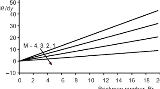
Figure 9(a). Rate of heat transfer (case II): at y = 1 (solid) and y = 0 (dotted) for variable Q
when M = 1, N = 1, α = 0.1, and k = 0.01
We now analyze the variation in the rate of heat transfer for the case II, figs. 6(b)- -9(b). In this case there is no heat transfer from the upper impermeable moving wall. The rate of heat transfer at the lower naturally permeable boundary is discussed. Figure 6(b) clearly in-dicates that as the permeability parameter k decreases, the rate of heat transfer at the lower
1
0.8
0.6
0.4
0.2
0
–0.5 0 0.5 1 1.5 2 2.5
Br ~ 0, = 10, 20, 30, 40, 50
y
Temperature, θ
0 5 10 15
Br = 50, 40, 30, 20, 10
y
0 0.1 0.2 0.3 0.4 0.5 0.6 0.7 0.8 0.9 1
Temperature, θ
Br ~0
K ~ 0, = 0.001, 0.01, 0.1
K ~ 0, = 0.001, 0.01, 0.1 6
4 2 0 –2 –4 –6 –8
0 2 4 6 8 10 12 14 16 18 20
Brinkman number, Br d /dθ y
M = 4, 3, 2, 1
M = 4, 3, 2, 1
Brinkman number, Br
0 2 4 6 8 10 12 14 16 18 20
10
5
0
–5
–10
–15
–20 d /dθ y
N = 1,2,3,4
N = 1,2,3,4
0 2 4 6 8 10 12 14 16 18 20
Brinkman number, Br 4
2
0
–2
–4
–6 d /dθ y
Q = 1, 2, 3, 4 Q = 1, 2, 3, 4
0 2 4 6 8 10 12 14 16 18 20
Brinkman number, Br 6
4
2
0
–2
–4
wall increases. Figure 7(b) unequivocally says that as the Hartmann number M increases the rate of heat transfer increases at the lower wall. Figure 8(b) indicates that with the increase in radiation parameter N the rate of heat transfer at the lower boundary decreases. It is clear from fig. 9(b) that as the heat source parameter Q increases, the rate of heat transfer increases at the lower permeable boundary.
Figure 6(b). Rate of heat transfer (no flux case) at the lower naturally permeable boundary (y = 0) for varying values of k when M = 1,
N = 1, α = 0.1, and Q = 1
Figure 7(b). Rate of heat transfer (no flux case) at the lower naturally permeable boundary (y = 0) for varying values of M when k = 0.01,
N = 1, α = 0.1, and Q = 1
Figure 8(b). Rate of heat transfer (no flux case) at the lower naturally permeable boundary (y = 0) when N varies when k = 0.01, M = 1,
α = 0.1, and Q = 1
Figure 9(b). Rate of heat transfer (no flux case) at the lower naturally permeable boundary (y = 0) when Q varies when k = 0.01, N = 1,
α = 0.1, and M = 1
Critical Brinkman number is that value of Brinkman number at which the heat transfer changes its direction. The variation of critical Brinkman number (CBr1) at the up-per wall (y = 1) for case I (isothermal case) with respect to various parameters is shown in tabs. 1-2.
Table 1 shows the effects of various parameters on CBr. When M = 0 = N = Q = k
then CBr comes out to be 2.0402. Here k → 0 corresponds to impermeable bottom. When permeable boundary is introduced, and k = 0.01, M = 0 = Q = N then CBr attains the value 8. The effect of Lorentz force is to decrease CBr as we see that when M = 1 and other parame-ters are zero, CBr reduces to 1.2324 as compared to its value 2.0402 when all parameparame-ters are zero. From this table it is also clear that the introduction of radiation enhances the CBr value while the introduction of heat source parameter Q causes decay in CBr.
k ~ 0, = 0.001, 0.01, 0.1
0 2 4 6 8 10 12 14 16 18 20 Brinkman number, Br 14
12 10 8 6 4 2 0 –2 d /dθ y
M = 4, 3, 2, 1
0 2 4 6 8 10 12 14 16 18 20
Brinkman number, Br 50
40
30
20
10
0
–10 d /dθ y
N = 1, 2, 3, 4
0 2 4 6 8 10 12 14 16 18 20
Brinkman number, Br 10
8
6
4
2
0 d /dθ y
Q = 4, 3, 2, 1
0 2 4 6 8 10 12 14 16 18 20
Brinkman number, Br 25
20
15
10
5
0
Tables 2 and 3 display the values of CBr for nu-merous cases of varying values of the parameters. Table 2 displays the variation in CBr with respect to M and N
when k = 0.01, Q = 1 The table shows that when M = 0 and N = 1, CBr = 15.3479 but as soon as the magnetic field is introduced with strength M = 1, CBr dips drasti-cally to 3.4090 and decreases further with increasing val-ues of M. When N = 0 and other parameters are non-zero CBr = 1.0570 but as radiation is introduced with strength
N = 1, CBr increases to 3.4090 which further increases with the increasing values of k. Table 3 displays the effect of permeability parameter k and heat source Q on CBr. It is evident from the table that as Q increases CBr decreas-es while CBr increasdecreas-es with the increasing valudecreas-es of k.
Conclusions
The main objective of the present work is to inves-tigate the effects of permeable boundary on the radiative heat transfer with dissipative effects relative to the heat flow resulting from the impressed temperature difference of the channel walls. On the basis of this study we may conclude following:
● The naturally permeable boundary has a significant impact on the momentum and thermal regime. ● As the strength of the magnetic field increases the
effect of permeability on the fluid velocity, fluid temperature, rate of heat transfer and critical Brinkman number becomes insignificant and the fluid flows within the channel as if no permeable boundary is present.
● Increased magnetic field parameter retards the flow. As we increase the permeability parameter the ve-locity of the fluid increases.
● For both cases (I and II) when the upper wall is iso-thermal/adiabatic we infer:
– On increasing the permeability parameter both the fluid temperature and θ′(0) decrease. – On increasing the Hartmann number both the
fluid temperature and θ′(0) increase.
– With the increase in radiation parameter both the temperature and θ′(0) decrease.
– With the increase in source parameter both the temperature and θ′(0) increase.
– As we increase the Brinkman number a rise in the fluid temperature is observed.
● For case I, when the channel walls are isothermal we infer that:
Table 1. Variation in CBr (isothermal case)
M N Q k CBr
0 0 0 0 2.0402
0 0 0 0.01 8.0000
1 0 0 0 1.2324
0 1 0 0 4.7605
0 0 1 0 1.1828
Table 2. Variation in CBr (isothermal case) with M and N
when k = 0.01, and Q = 1
M N CBr
0 1 15.3479
1 1 3.4090
2 1 1.3055
3 1 0.7839
4 1 0.5608
1 0 1.0570
1 2 5.7587
1 3 8.1079
1 4 10.4569
Table 3. Variation in CBr (isothermal case) with M and N
when M = 1, and N = 1
K Q CBr
0 1 2.3983
0.001 1 2.8093
0.01 1 3.4090
0.1 1 3.8306
0.2 1 3.9062
0.01 0 4.1104
0.01 2 2.7028
0.01 3 1.9913
– On increasing the permeability and radiation parameter both θ′(1) and CBr in-crease.
– On increasing Hartmann number and heat source parameter θ′(1) and CBr, both decrease.
– With the increase in heat source parameter, both θ′(1) and CBr decrease.
Nomenclature
B – constant, [–]
B0 – uniform transverse magnetic field, [T] Br – Brinkman number
Case I = µ(u1) 2
/κ(T1 – T0), and Case II = µ(u1)
2
/(κT0), [–] g – gravitational acceleration, [ms–2] h – channel width, [m]
k – permeability, [m2]
k* – dimensionless permeability, [–] k1 – mean absorption coefficient, [m –1
] M – Hartmann number [= ( B0
2
h2/µ)–1/2], [–] N – radiation parameter
{ = [4 1(Tm) 3
]/(k1κ)}, [–] p – fluid pressure, [kg m–1s–2] p0 – constant pressure at origin, [kg m
–1 s–2] Q – heat source parameter (= Q0h
2 /κ), [–] Q0 – uniform heat source
qr – radiation heat flux
[= (–4 1/3k1)(∂T 4
/∂y)], [ kgm–2] T – fluid temperature, [K]
T0 – temperature of lower permeable boundary, [K]
T1 – temperature of upper wall for case I, [K]
u, v, w – velocity components along x-, y-, and z- directions, respectively, [ms–1]
u*, v*, w* – dimensionless velocity compo-nents, [–]
u1 – velocity of upper wall, [ms –1
] x – Cartesian co-ordinate along the
permeable boundary, [m] x*, y*, z* – dimensionless Cartesian
co-ordi-nates, [–]
y – Cartesian co-ordinate along the width of the channel, [m] z – Cartesian co-ordinate normal to
the channel, [m]
Greek symbols
α – empirical constant, [–]
θ – dimensionless fluid temperature, [K] µ – dynamic viscosity, [Nsm–2] κ – thermal conductivity, [kgms–3K–1] ρ – fluid density, [kgm–3]
– electrical conductivity, [Sm–1]
σ1 – Stefan Boltzmann constant, [kgm –2
K–4] References
[1] Leadon, B. M., Plane Couette Flow of a Conducting Gas through a Transverse Magnetic Field, Convair Scientific Research Laboratory,San Diego, Cal., USA, Research note No. 13, 1957
[2] Verma, P. D., Bhatt, B. S., Plane Couette Flow of Two Immiscible Incompressible Fluids with Uniform Suction at the Stationary Plate, Proceedings Mathematical Science, 78 (1973), 3, pp. 108-120
[3] Chauhan, D. S., Vyas, P., Heat Transfer in Hydromagnetic Couette flow of Compressible Newtonian Fluid, ASCE Journal of Engineering Mechanics, 121 (1995), 1, pp. 57-61
[4] Kuznetsov, A. V., Analytical Investigation of Couette Flow in a Composite Channel Partially Filled with a Porous Medium and Partially with a Clear Fluid, Int. J. of Heat Mass Transfer, 41 (1998), 16, pp. 2556-2560
[5] Chauhan, D. S., Kumar, V., Heat Transfer Effects in a Couette Flow through a Composite Channel Par-tially Filled by a Porous Medium with a Transverse Sinusoidal Injection Velocity and Heat Source, Thermal Science, 15 (2011), Suppl. 2, pp. S175-S186
[6] Berman, A. S., Laminar Flow in Channels with Porous Walls, J. Appl. Phys., 24 (1953), 9, pp. 1232-1235
[7] Beavers, G. S., Joseph, D. D., Boundary Conditions at a Naturally Permeable Wall, J. Fluid Mech., 30 (1967), 1, pp. 197-207
[8] Taylor, G. I., A Model for the Boundary Condition of a Porous Material, Part 1, J. Fluid Mech., 49 (1971), 2, pp. 319-326
[9] Richardson, S., A Model for the Boundary Condition of a Porous Material, Part 2, J. Fluid Mech., 49 (1971), 2, pp. 327-336
[11] Sahraoui, M., Kaviany, M., Slip and no-Slip Velocity Boundary Conditions at the Interface of Porous Plain Media, Int. J. Heat Mass Transfer, 35 (1992), 4, pp. 927-943
[12] Vafai, K., Kim, S. J., Fluid Mechanics of the Interface Region between a Porous Medium and a Fluid Layer – An exact solution, Int. J. Heat Fluid Flow, 11 (1990), 3, pp. 254-256
[13] Klikenberg, L. J., The Permeability of Porous Media to Liquids and Gases, Drilling and Production Practices, American Petroleum Institute, Washington, DC., USA, 1941, pp. 200-213
[14] Saffman, P. G., On the Boundary Condition at the Surface of a Porous Medium, Studies in Applied Ma-thematics, L (1971), 2, pp. 93-101
[15] Makinde, O. D., Osalusi, E., MHD Steady Flow in a Channel with Slip at the Permeable Boundaries, Rom. Journ. Phys., 51 (2006), 3-4, pp. 319-328
[16] Singh, R. K., et al., On Hydromagnetic free Convection in the Presence of Induced Magnetic Field, Heat and Mass Transfer, 46 (2010), 5, pp. 523-529
[17] Nikodijevic, D., et al., MHD Couette Two-Fluid Flow and Heat Transfer in Presence of Uniform In-clined Field, Heat and Mass Transfer, 47 (2011), 12, pp. 1525-1535
[18] Viskanta, R., Heat Transfer in a Radiating Fluid with Slug Flow in a Parallel Plate Channel, Applied Scientific Research, 13 (1964), 1, pp. 291-311
[19] Helliwell, J. B., On the Stability of Thermally Radiative Magnetofluiddynamic Channel Flow, Journal of Engineering Mathematics, 11 (1977), 1, pp. 67-80
[20] Elsayed, M. M., Fathalah, K. A., Simultaneous Convection and Radiation in Flow between Two Paral-lel Plates, Int. J. of Heat and Fluid Flow, 3 (1982), 4, pp. 207-212
[21] Helliwell, J. B., Mosa, M. F., Radiative Heat Transfer in Horizontal Magnetohydrodynamic Channel Flow with Buoyancy Effects and an Axial Temperature Gradient, Int. J. Heat Mass Transfer, 22 (1979), 5, pp. 657-668
[22] Elbashbeshy, E. M. A., Emam, T. G., Effects of Thermal Radiation and Heat Transfer over an Unstea-dy Stretching Surface Embedded in a Porous Medium in the Presence of Heat Source or Sink, Thermal Science, 15 (2011), 2, pp. 477-485
[23] Gebhart, B., Effect of Viscous Dissipation in Natural Convection, J. Fluid Mech., 38 (1962), 2, pp. 225-232
[24] Gebhart, B., Mollendorf, J., Viscous Dissipation in External Natural Convection Flows, J. Fluid Mech., 38(1969), 1, pp. 97-107
[25] Magyari, E., Keller, B., The Opposing Effects of Viscous Dissipation Allows for a Parallel Free Con-vection Boundary-Layer Flow along a Cold Vertical Flat Plate, Transp. Porous Media, 51 (2003), 2, pp. 227-230
[26] Rees, D. A. S., et al., The Development of the Asymptotic Viscous Dissipation Profile in a Vertical Free Convective Boundary Layer Flow in a Porous Medium, Transp. Porous Media, 53 (2003), 3, pp. 227-230
[27] Illingworth, C. R., Some Solutions of the Equations of Flow of a Viscous Compressible Fluid, Proc. Cambr. Phil. Soc., 46 (1950), 3, pp. 469-478
[28] Morgan, A. J. A., On the Couette Flow of a Compressible Viscous, Heat Conducting, Perfect Gas, JAS, 24 (1957), April, pp. 315-316
[29] Modest, M. F., Radiative Heat Transfer, 2nd ed., Academic Press, New-York, USA, 2003