Convective Heat And Mass Transfer Flow Of A Micropolar Fluid In A Rectangular Duct With Soret And Dufour Effects And Heat Sources

Convective Heat And Mass Transfer Flow Of A Micropolar Fluid

In A Rectangular Duct With Soret And Dufour Effects And Heat

Sources

C.Sulochana

a

, K. Gnanaprasunamba

b

*

a

Department of Mathematics, Gulberga University, Gulberga, Karnataka, India

b

Department of Mathematics, SSA Govt. First Grade College, Bellary, Karnataka, India

Abstract

In this chapter we make an investigation of the convective heat transfer through a porous medium in a Rectangular enclosure with Darcy model. The transport equations of liner momentum, angular momentum and energy are solved by employing Galerkine finite element analysis with linear triangular elements. The computation is carried out for different values of Rayleigh number – Ra micropolar parameter – R, spin gradient parameter, Eckert number Ec and heat source parameter. The rate of heat transfer and couple stress on the side wall is evaluated for different variation of the governing parameters.

Keywords:

Heat and Mass Transfer, Micropolar Fluid, Soret and Dufour Effect, Rectangular Duct

I.

INTRODUCTION

As high power electronic packaging and component density keep increasing substantially with the fast growth of electronic technology, effective cooling of electronic equipment has become exceptionally necessary. Therefore, the natural convection in an enclosure has become increasingly important in engineering applications in recent years. Through studies of the thermal behavior of the fluid in a partitioned enclosure is helpful to understand the more complex processes of natural convection in practical applications Number of studies, numerical and experimental, concerned with the natural convection in an enclosure with or without a divider were conducted in past years.

Several relevant analytical and experimental studies have been reported during the past decades. Excellent reviews have been given by Ostrach [17] and Catton [2]. The critical Rayleigh numbers for natural convection in rectangular boxes heated from below and cooled from above have been obtained theoretically by Davis [7] and Cotton [4]. Samuels and Churchill [20] presented the stability of fluids in rectangular region heated from below and obtained the critical Rayleigh numbers with finite differences approximation. Ozoe et. al., [18,19] determined experimentally and numerically the natural convection in an inclined long channel with a rectangular cross-section, and found the effects of inclination angle and aspect ratio on the circulation and rate of heat transfer, Wilson and Rydin [22] discussed bifurcation phenomenon in a rectangular cavity, as calculated by a nodal integral method. They obtained critical aspect ratios and Rayleigh numbers and found good agreement with the results of Ref [5]. Numerous studies have been presented for a different arrangement of boundary conditions [14-15]. Several analytical studies of natural heat transfer in a rectangular porous cavity have been carried out recently [1, 2]. The theory of micropolar fluids developed by Erigen [8, 9, 11] has been a popular filed of research in recent years. In this theory, the local effects arising from the microstructure and the intrinsic motions of the fluid elements are taken into account. It has been expected to describe properly the non-Newtonian behavior of certain fluids, such as liquid crystals, ferroliquids, colloidal fluid, and liquids with polymer additives. Recently Jena and Bhattacharya [13] studied the effect of microstructure on the thermal

convection in a rectangular box heated from below wit Galerkin’s method, and obtained critical Rayleigh

numbers for various material parameters, Cehn and Hsu [6] considered the effect of mesh size on the thermal convection in an enclosed cavity. Wang et.al., [24] presented the study of the natural convection of micropolar fluids in an inclined rectangular enclosure, HSU et. al., [24] investigated the thermal convection of micropolar fluids in a lid-driven cavity. They reported that the material parameters such as voters viscosity and sin gradient viscosity strongly influence the flow structure and heat transfer. Cha-Kaungchen et. al., [6] have investigated numerically the steady laminar natural convection flow of a micropolar fluid in a rectangular cavity. The angular momentum and energy are solved with the aid of the cubic spline collocation method. Parametric studies of the effects of microstructure on the fluid flow and heat transfer in the enclosure have been performed.

Wang et. al., (23) have investigated natural convection flow of a micropolar fluid in a partially divided rectangular enclosure. The enclosure is partially divided protruding flore of the enclosure. The effect of the highest on the location of the divider is investigated. Also the effects of material parameters or micropolar fluids or the thermal characters, are also studied for different Rayleigh numbers. Tsan – Hsu et. al., (6) have investigated the effects, the characteristic parameters of micropolar fluids on mixed convection in a cavity. The equations are solved with the help of the cubic spin collocation method.

In this chapter we make an investigation of the convective heat transfer through a porous medium in a Rectangular enclosure with Darcy model. The transport equations of liner momentum, angular momentum and energy are solved by employing Galerkine finite element analysis with linear triangular elements. The computation is carried out for different values of Rayleigh number – Ra micropolar parameter – R, spin gradient parameter, Eckert number Ec and heat source parameter. The rate of heat transfer and couple stress on the side wall is evaluated for different variation of the governing parameters.

II.

FORMULATION OF THE PROBLEMS

We consider the mixed convective heat and mass transfer flow of a viscous, incompressible, micropolar fluid in a saturated porous medium confined in the rectangular duet whose base length is a and height b. the heat flux on the base and top walls is maintained constant. The Cartesian coordinate system 0(x, y) is chosen with origin on the central axis of the duct and its base parallel to X-axis, we assume that

(i) The convective fluid and the porous medium are everywhere in local thermodynamic equilibrium. (ii) There is no phase change of the fluid in the medium.

(iii) The properties of the fluid and of the porous medium are homogeneous and isotropic.

(iv) The porous medium is assumed to be closely packed so that Darcy’s momentum law is adequate in the porous medium.

(v) The Boussinesq approximation is applicable,

under the assumption the governing equations are given by

0





















y

v

x

u

(2.1)

0

)

(

1



















y

N

k

u

k

k

x

p



(2.2)

0

)

(

1





















g

y

N

k

v

k

k

y

p



_

(2.3)































































2 2 2 2

y

T

x

T

k

y

T

v

x

T

u

C

_{P f}





(2.4)





















































































N

y

u

x

v

K

y

N

x

N

y

N

v

x

N

u

j 2

2

2

2 2





(2.5)























































2 2 2 2

y

C

x

C

D

y

C

v

x

C

u

C

_{P m}





(2.6)

)}

(

)

(

1

{

_{0 0 0}

0



T



T



C



C





_

_

_





2

0 c h

T

T

T





,

2

0

c

h

C

C

C





(2.7)

where u and v are Darcy velocities along 0(x, y) direction. T, N, p and g are the temperature, micro rotation, pressure and acceleration due to gravity, Tc and Th are the temperature on the cold and warm side walls

respectively. , , v and  are the density, coefficients of viscosity, kinematic viscosity and thermal expansion of the fluid, k1 is the permeability of the porous medium, , k are the micropolar and material constant pressure ,

Q is the strength of the heat source,k11&k2

is the cross diffusivities,1 is the chemical reaction parameter, The boundary conditions are

T = Th ,C=Ch on the side wall to the right (x = 1)

T = Tc ,C=Cc on the side wall to the right (x = 0) (2.7)

0









y

T

,



0





y

C

on the top (y = 0) and bottom

u = v = 0 walls (y = 0) which are insulated,

x

u

N









2

1

On y = 0 & 1

x

v

N









2

1

On x = 0 & 1 (2.8)

Eliminating the pressure p from equations (2.2) & (2.3) and using (2.6) we get

)

(

)

(

(

)

(

0

_{2 0 0}

2 2 2 1

C

C

x

g

T

T

x

g

x

v

y

u

k

x

v

y

u

k

k













































































(2.11)

On introducing the stream function, as

y

u











,

y

v









the equations (2.11) & (2.5) reduce to

))

C

-(C

)

T

-(T

(

)

(

0 0 0 2 2 1

x

g

x

g

N

k

k

k























_

_





(2.12)

T

k

y

T

y

y

T

x

C

_{P f} 2

0









































(2.13)



N



K

N

x

y

y

x

j

2

2

2

_

_

_











































_

_



(2.14)

C

D

y

C

y

y

C

x

m 2







































(2.15)

Now introducing the following non-dimensional variables

ax

x





:

y





by

:

a

b

C



,

v







u

a

v

u

















:

v

a

v

v

















:

p

a

v

p

_















2 2



T = Tc + (Th– Tc):

























22

a

v

N

N

C = Cc + C (Ch– Cc): (2.16)

the equations (2.12) – (2.14) in the non-dimensional form are



























































2 2 2 2 2

y

N

x

y

y

y

x

P









(2.18)



































2 2

2









R

R

(2.19)



























































2 2 2 2

y

C

x

C

y

C

y

y

C

x

Sc

(2.20)

where 2 3

)

(

v

a

T

T

g

G

 

h



c

(Grashof number)

f p

k

C

P





/

(Prandtl number)

1 2 1

k

a

D





(Darcy parameter)



k

R



(Micropolar parameter)

2

va







(Micropolar material constant)

m

D

Sc





(Schmidt number)

)

(

)

(

c h c h

T

T

C

C

N













(Buoyancy ratio)

And the corresponding boundary conditions are

y = x = 0 on the boundary (2.18a)

 = 1 , C=1 on x = 1 (2.18b)

 = 0 , C=0 on x = 0

y

x

N











2

2

1

On y = 0 & 1

x

y

N













2

2

1

On x = 0 & 1 (2.18c)

III.

FINITE ELEMENT ANALYSIS AND SOLUTION OF THE PROBLEM

The region is divided into a finite number of three noded triangular elements, in each of which the element equation is derived using Galerkin weighted residual method. In each element fi the approximate solution for an

unknown f in the variation formulation is expressed as a linear combination of shape function

 

N

ki k = 1, 2, 3,

which are linear polynomials sin x and y. This approximate solution of the unknown f coincides with actual values of each node of the element. The variation formulation results in 3x3 matrix equation (stiffness matrix) for the unknown local nodal values of the given element. The stiffness matrices are assembled in terms of global nodal values using inter element continuity and boundary conditions resulting in global matrix equation.

In each case there are r district global nodes in the finite element domain and fp = (p =1, 2.r) is the global

Then



 





s r

p p p

f

f

1 1



Where the first summation denotes summation over s elements and the second one represents summation over the independent global nodes and

i N i p



N



, if p is one of the Local nodes say k of the element ei = 0,

p

f



s are determined from the global matrix equation. Based on these lines we now make a finite element analysis of the given problem governed by (2.15) – (2.17) subject to the conditions (2.18a) – (2.18c).

Let i, i and Ni be the approximate values,  and N in a element ei

i i i i i i i

N

N

N

₁



₁



₂



₂



₃



₃





(3.1a) i i i i i i i

N

N

N

₁



_{1 2}



_{2 3}



₃









(3.1b)

i i i i i i i

C

N

C

N

C

N

C



1 1



2 2



3 3 (3.1c)

i i i i i

N

N

N

N

i

N

N



1



2



3 (3.1d)

Substituting the approximate value iI, Ci and i for, , C and  respectively in (2.15)





























































y

x

x

y

P

y

x

E

i i i i i i

i









2 2 2 2 1 (3.2)











































2 ₂ 2 ₂ 2 ₂ 2 ₂

2

2

y

x

R

R

y

x

E

i i i i i i









(3.3)

Under Galaerkin method this is made orthogonal over the domain ei to the respective shape functions (weight

function)

Where







i e i k i

d

N

E

₁

0







i e i k i

d

N

E

₂

0

(3.4) 2

)

0

2 2 2



































































d

y

x

x

y

P

y

x

N

i i i i i i i e u k i









0

2

₂ 2 2 2 2 2 2 2



























































d

y

x

R

R

y

x

N

i i i i i e i k i









(3.5)

Using Greeen’s theorem we reduce the surface integral (3.4) & (3.5) without affecting  terms and obtain























































































 



y

y

PN

y

x

x

y

d

N

x

x

N

N

N

i i i i k i i k i i k e i k i









3

4

1































i i i i i

k

ny

d

x

nx

x

N





(3.6)















































































R

R

N

_x

_x

N

_y

_y

i i i i i e i

k

ny

d

y

R

y

nx

x

R

x

N

i



























































































(3.7)

Where 1 is the boundary of ei, substituting L.H.S of (3.1a) – (3.1c) for i, i and Ni in (3.6) & (3.7) we get

y

N

y

N

x

N

x

N

N

i k i L i L i k e i i





































 1 3 1

3

4

1



































 



y

N

x

N

x

N

y

N

P

i L i m i L i m i e i m i 3 1 1 i k i i i i

k

ny

d

W

y

nx

x

N

i





































(l, m, k = (1, 2, 3) (3.8)

y

N

y

N

x

N

x

N

_ki _Li _Li _ki

e

i _i























 3 1



































 



y

N

x

N

x

N

y

N

Sc

i L i m i L i m i e i m i 3 1

0

)

(



















d

dx

dN

dx

dN

dx

dN

dx

dN

ScSr

d

N

N

C

k

ei i L i m i L i k i e i i l i k i c i



i k i i i i

k

ny

d

W

y

nx

x

N

i





























_







(

(l, m, k = (1, 2, 3)

N i i i i i i k i J i k i J i k i i L i k i e i k i L i L i k i

Q

d

ny

y

R

R

y

nx

x

R

x

N

d

y

N

y

N

x

N

x

N

R

d

N

N

R

y

N

y

N

y

N

x

N

N

i i

















































































































































































2 1

2

(3.9)

Where

Q

Q

Q

Q

Q

ki

s

i k i k i k i

k



1



2



3

,

'

being the values of i k

Q

on the sides s = (1, 2, 3) of the element ei. The

sign of

Q

ki’s depends on the direction of the outward normal with reference to the element.

Choosing different

N

ki’s as weight functions and following the same procedure we obtain matrix

equations for three unknowns

(

Q

ip

)

)

(

)

)(

(

ki

i p i

p

Q

Q

Where

(

Q

ipk

)

3 x 3 matrixes are,

(

),

(

)

i i

p

Q

Q

are column matrices.

Repeating the above process with each of s elements, we obtain sets of such matrix equations. Introducing the global coordinates and global values for

(

Q

i_p

)

and making use of inter element continuity and boundary conditions relevant to the problem the above stiffness matrices are assembled to obtain a global matrix equation. This global matrix is rxr square matrix if there are r distinct global nodes in the domain of flow considered.

Similarly substituting i i ,i , and i in (2.12) and defining the error and following the Galerkin method we obtain using Green’s Theorem, (3.8) reduces to









       

















































































































































nxd

N

GD

d

ny

y

N

ny

x

N

RD

d

ny

y

nx

x

d

y

N

y

N

x

N

x

N

RD

x

N

GD

y

y

N

x

x

N

i k i i i k i i i i k i i k i k i i k i i k 1 1 1 1

.



(3.9)

in obtaining (3.9) the Green’s Theorem is applied with reference to derivatives of  without affecting  terms. Using (3.1-3.1c) in (3.9) we have











_

































































    m i L i k i L i L i k L i L i k i m i m i k i m

d

x

N

N

d

x

N

N

GD

d

y

N

y

N

x

N

x

N

1 2 2

)

(

)

(

2

(







i

k

d

N

d

ny

y

N

y

nx

x

N

x

N

i i _i

k i i i i i k





























































































(3.10)

In the problem under consideration, for computational purpose, we choose uniform mesh of 10 triangular elements. The domain has vertices whose global coordinates are (0, 0), (1, 0) and (1, c) in the non-dimensional form. Let e1, e2…..e10 be the ten elements and let 1, 2,….10 be the global values of  and 1, 2….10 are the

global values of  at the global nodes of the domain.

IV.

SHAPE FUNCTIONS AND STIFFNESS MATRICES

x

n

3

1

1

,

1





h

y

x

n

3

3

2

,

1





h

y

n

3

1

1

,

2





h

y

n

3

1

2

,

2







h

y

x

n

3

3

1

3

,

2







x

n

3

2

1

,

3





h

y

x

n

3

3

1

2

,

3









h

y

n

3

3

,

3





C

y

n

₃

1

1

,

4





x

n

3

2

2

,

4







h

y

x

n

3

3

2

3

,

4







x

n

3

2

1

,

h

y

x

n

3

3

1

2

,

5









h

y

n

3

3

,

5



h

y

n

3

1

3

,

6





h

y

n

3

2

1

,

7





x

n

3

2

2

,

7







h

y

x

n

3

3

1

3

,

7







x

n

3

3

1

,

8





h

y

x

n

3

3

1

2

,

8









h

y

x

n

3

3

2

,

9





h

y

n

3

1

3

,

9







The global matrix for  is

A3 X3 = B3 (4.1)

The global matrix for N is

A4 X4 = B4 (4.2)

The global matrix  is

A5 X5 = B5 (4.3)

The domain consists three horizontal levels and the solution for Ψ, θ and N at each level may be expressed in terms of the nodal values as follows,

In the horizontal strip 0 ≤y ≤

3

h

Ψ= (Ψ1N11+ Ψ2N12+ Ψ7N17) H (1- τ1)

= Ψ1 (1-4x)+ Ψ2

4(x-h

y

)+ Ψ7 (

h

y

4

(1- τ1 ) (0≤ x≤

3

1

)

Ψ =( Ψ2N32+ Ψ3N33+ Ψ6N36) H(1-τ2)

+ (Ψ2N22+ Ψ7N27+ Ψ6N26)H(1- τ3) (

3

1

≤ x≤

3

1

)

=( Ψ22(1-2x) + Ψ3

(4x-h

y

4

-1)+ Ψ6 (

h

y

4

))H(1-τ2)

+( Ψ2

(1-h

y

4

)+ Ψ7 (1+

h

y

4

-4x)+ Ψ6 (4x-1))H(1- τ3)

Ψ =( Ψ3N 5

3+ Ψ4N 5

4+ Ψ5N 5

5) H(1- τ3)

+ (Ψ3N 4

3+ Ψ5N 4

5+ Ψ6N 4

6)H(1- τ4) (

3

2

≤ x≤1)

=( Ψ3 (3-4x) + Ψ4

2(2x-h

y

2

-1)+ Ψ6 (

h

y

4

-4x+3))H(1- τ3)

+ Ψ3

(1-h

y

4

)+ Ψ5 (4x-3)+ Ψ6 (

h

y

4

))H(1- τ4)

Along the strip

3

h

≤ y≤

3

2

h

Ψ =( Ψ7N 6

7+ Ψ6N 6

6+ Ψ8N 6

8) H(1-τ2) (

3

1

≤ x≤1)

+( Ψ6N76+ Ψ9N79+ Ψ8N78) H(1- τ3)+( Ψ6N86+ Ψ5N85+ Ψ9N89) H(1- τ4)

Ψ =( Ψ7 2(1-2x) + Ψ6 (4x-3)+ Ψ8 (

h

y

4

-1))H(1- τ3)

+ Ψ6

(2(1-h

y

2

)+ Ψ9 (

h

y

4

-1)+ Ψ8 (1+

c

y

4

-4x))H(1- τ4)

+ Ψ6 (4(1-x)+ Ψ5

(4x-c

y

4

-1)+ Ψ92(

h

y

2

-1))H(1- τ5)

Along the strip

3

2

h

≤ y≤1

Ψ = ( Ψ8N98+ Ψ9N99+ Ψ10N910) H(1-τ6) (

3

2

≤ x≤1)

= Ψ8 (4(1-x)+ Ψ9

4(x-h

y

)+ Ψ102(

h

y

4

-3))H(1-τ6)

where τ1= 4x , τ2 = 2x , τ3 =

3

4

x

,

τ4=

4(x-h

y

), τ5=

2(x-h

y

), τ6 =

3

4

(x-h

y

)

And H represents the Heaviside function.

In the horizontal strip 0≤ y≤

3

h

θ = [θ1 (1-4x) + θ2

4(x-h

y

) + θ7 (

h

y

4

)) H (1- τ1) (0≤ x≤

3

1

)

θ = (θ 2(2(1-2x) + θ3

(4x-c

y

4

-1) + θ 6(

c

y

4

)) H (1-τ2)

+ θ 2(1-

h

y

4

) + θ 7(1+

h

y

4

-4x) + θ 6(4x-1)) H (1- τ3) (

3

1

≤ x≤

3

2

)

θ = θ 3(3-4x) +2 θ 4

(2x-h

y

2

-1) + θ 6(

h

y

4

-4x+3) H (1- τ3)

+ (θ 3(1-

h

y

4

) + θ 5(4x-3) + θ 6(

h

y

4

)) H (1- τ4) (

3

2

≤ x≤1)

Along the strip

3

h

≤ y≤

3

2

h

θ = (θ 7(2(1-2x) + θ 6(4x-3) + θ 8(

h

y

4

-1)) H (1- τ3) (

3

1

≤ x≤

3

2

)

+ (θ 6(2(1-

h

y

2

) + θ 9(

h

y

4

-1) + θ 8(1+

h

y

4

-4x)) H (1- τ4)

+ (θ 6(4(1-x) + θ 5

(4x-h

y

4

-1) + θ9 2(

h

y

4

-1)) H (1- τ5)

Along the strip

3

2

h

≤ y≤1

θ = (θ84(1-x) + θ 94(x-

h

y

)+ θ 10(

h

y

4

-3) H(1-τ6) (

3

2

≤ x≤ 1)

The expressions for N are

N = [N1(1-4x)+ N2

4(x-c

y

)+ N7 (

c

y

4

)) H(1- τ1) (0≤ x≤

3

1

)

N = (N 2(2(1-2x)+ N3

(4x-h

y

4

-1)+ N 6(

h

y

4

)) H(1-τ2)

+ N 2

(1-h

y

4

)+ N7(1+

h

y

4

-4x)+ N 6(4x-1))H(1- τ3) (

3

1

≤ x≤

3

2

)

N = N3(3-4x) +2 N4

(2x-h

y

2

-1)+ N6(

h

y

4

-4x+3) H(1- τ3)

+( N3

(1-h

y

4

)+ N5(4x-3)+ N6(

h

y

4

)) H(1- τ4) (

3

2

≤ x≤1)

Along the strip

3

h

≤ y≤

3

2

h

N = (N7(2(1-2x)+ N6(4x-3)+ N8(

c

y

4

-1)) H(1- τ3) (

3

1

≤ x≤

3

2

)

+( N6

(2(1-h

y

2

)+ N9(

h

y

4

-1)+ N8(1+

h

y

4

-4x)) H(1- τ4)

+( N6(4(1-x)+ N5

(4x-h

y

4

-1)+ N9 2(

h

y

4

Along the strip

3

2

h

≤ y≤1

N = (N84 (1-x) + N94(x-

h

y

)+ N10 (

h

y

4

-3) H(1-τ6) (

3

2

≤ x≤ 1)

The dimensionless Nusselt numbers on the non-insulated boundary walls of the rectangular duct are calculated using the formula

Nu = (

x







) x=1

Nusselt number on the side wall x=1 in the different regions are

Nu1 = 2-4 θ3, 3

*

1

2

4

N

M





0≤ y≤

3

c

Nu2= 2-4 θ6 6 *

2

2

4

N

M





3

c

≤ y≤ 2

3

c

Nu3 = 2-4 θ9, 9 *

3

2

4

N

M





3

2

c

≤ y≤1

The details of a11, b11, ar1, br1, cr1 etc., are shown in appendix

The equilibrium conditions are

0

2 1 1

3



R



R

, 13

0

2

3



R



R

0

4 1 3

3



R



R

,

R

₃4



R

₁5



0

0

2 1 1

3



Q



Q

,

Q

₃2



Q

₁3



0

0

4 1 3

3



Q



Q

, 15

0

4

3



Q



Q

0

2 1 1

3



S



S

, 13

0

2

3



S



S

0

4 1 3

3



S



S

, 15

0

4

3



S



S

4.4

Solving these coupled global matrices for temperature, Micro concentration and velocity (4.1 – 4.3) respectively and using the iteration procedure we determine the unknown global nodes through which the temperature, Micro rotation and velocity of different intervals at any arbitrary axial cross section are obtained.

V.

DISCUSSION

In this analysis we investigate the effect of dissipation and heat sources on convective heat and mass transfer flow of a micropolar fluid through a porous medium in a rectangular duct. The non-linear coupled equations governing the flow, heat and mass transfer have been solved by using Galerikin finite element analysis with three nodded triangular elements and Prandtl number Pr is taken as 0.71.

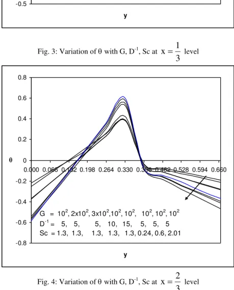
The non-dimensional temperature ‘’ is exhibited in fig 1-12 for different values of G, D-1, Sc, N,, Ec, R &  at different levels. We follow the convention that, the non-dimensional temperature is positive or negative according as the actual temperature is greater/smaller than the equilibrium temperature.

Figs. (1-4) represent  with G, D-1 & Sc. It is found that an increase in G enhances the actual temperature at

3

2

h

y



level,

3

1



x

&

3

2



x

levels and reduces at

3

h

y



level. With respect to Darcy parameter D-1, we

find the lesser the permeability of the porous medium larger the actual temperature at

3

2

h

y



,

3

1



x

&

3

2



x

levels and smaller at

3

h

y



level. The variation of  with Schmidt number Sc shows that lesser the

molecular diffusivity larger the actual temperature at

3

2

h

y



and

3

h

y



levels and smaller at

3

1



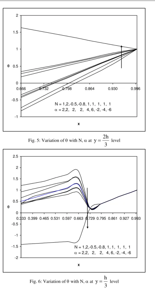
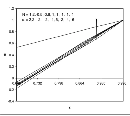
level an increase in Sc  0.6 enhances the actual temperature while it reduces with higher Sc  1.3 (figs 1-4).Figs (5-8) represent ‘’ with N &  at different levels. It is found that when the molecular buoyancy force

dominates over the thermal buoyancy force, the actual temperature enhances at

3

2

h

y



,

3

1



x

and

3

2



x

levels and reduces at

3

h

y



level when the buoyancy forces are in the same direction and for the forces acting

in the opposite directions, the actual temperature reduces at

3

2

h

y



,

3

h

y



,

3

1



x

levels and at

3

2



x

level, it enhances in the horizontal region (0  y  0.264) and reduces in the region (0.333  y  0.666).The

variation of with heat source parameter ‘’ shows that at

3

2

h

y



level, the actual temperature reduces with

 > 0 and enhances ||. At

3

h

y



level, the actual temperature reduces for  4 and enhances at higher  > 6

while it reduces || (fig. 5). At

3

1



x

level, the temperature enhances in the region (0, 0.067) and

reduces in the region (0.134, 0.333) for  4. For higher  6 the actual temperature reduces in the region (0, 0.201) and enhances in the region (0.268, 0.333). An increase in || leads to a depreciation in the actual

temperature (fig. 7). At

3

2



x

level, an increase in   4 reduces the actual temperature except in the

horizontal strip (0, 0.066) and for higher   6, the actual temperature increase in the region (0, 0.333) and reduces in the region (0.369, 0.666). An increase in || results in an enhancement in the actual temperature (fig. 8).Figs (9-12) represent  with Ec, R &. It is found that higher the dissipative heat larger the actual temperature

at

3

h

y



and

3

1



x

levels and smaller at

3

2

h

y



and

3

2



x

levels. An increase in micro rotation

parameter R reduces the actual temperature at

3

2

h

y



,

3

h

y



and

3

1



x

levels. At

3

2



x

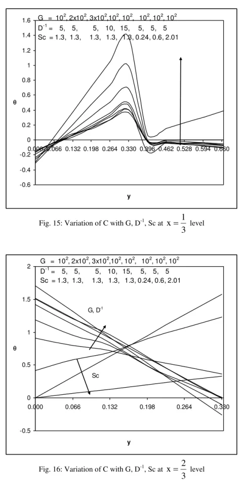
level the actual temperature enhances in the horizontal strip (0, 0.132) and reduces in the region (0.198, 0.666). An increase in the spin gradient parameter  leads to an enhancement in the actual temperature at all levels (figs 9-12).

The non-dimensional concentration (C) is shown in figs 13-24 for different parametric values. We follow the convention that the concentration is positive or negative according as the actual concentration is greater/lesser than the equilibrium concentration. Figs (13-16) represent the concentration. ‘C’ with G, D-1 & Sc.

It is found that the actual concentration enhances at

3

2

h

y



and

3

1



x

levels, while it reduces at

3

h

y



and

3

2



x

level. With reference to D-1 we find that lesser the permeability of the porous medium, larger the actual

concentration at

3

2

h

y



and

3

1



x

levels and smaller at

3

h

y



level. At

3

2



x

level the concentration reduces with D-1 in the horizontal strip (0, 0.333) and enhances in the region (0.369, 0.666). With reference to Sc, we find that lesser the molecular diffusivity smaller the actual concentration at both the horizontal levels. At

3

1



x

level the actual concentration enhances with Sc  0.6 in the region (0, 0.134) and reduces in the region

(0.201, 0.333) and for higher Sc  1.3, we notice a depreciation everywhere in the region except in the region (0, 0.666) (figs 13-16).

higher  6. An increase in the strength of heat absorbing source ||(<0) enhances the actual concentration at

both the horizontal levels. At

3

1



x

level, the actual concentration enhances in the region (0, 0.134) and

reduces in the region (0.201, 0.333) with  4 and for higher  6; we notice an enhancement in the actual

concentration. At

3

2



x

level the actual concentration reduces with  in the region (0, 0.132) and enhances in the region (0.201, 0.666) (figs 17-20).

Figs (21-24) represents the concentration with Ec, R and. It is found that higher the dissipative heat smaller the

actual concentration at both the horizontal levels and larger at

3

1



x

level. At

3

2



x

level, higher the dissipative heat larger the actual concentration in the region (0, 0.264) and smaller in the region (0.333, 0.666). An increase in R enhances the actual concentration at all levels. An increase in spin gradient parameter  leads

to the depreciation at both the horizontal levels and at

3

2



x

level, while it enhances at

3

1



x

level. (Figs

21-24).

Figs 25-28 represent micro rotation (  )with different value of G, D-1 & Sc. It is found that at

3

h

y



,

3

1



x

&

3

2



x

levels, the micro-rotation enhances with increasing G  2102 and reduces for G  3102

while at

3

2

h

y



level, the micro rotation enhances with G. With respect to D-1, we find that the micro rotation

reduces with D-1 10 and enhances with D-1 15 at

3

h

y



,

3

1



x

&

3

2



x

levels, while it enhances with D

-1

, at

3

2

h

y



level, The variation on  with Schmidt number Sc shows that lesser the molecular diffusivity

smaller the micro rotation at

3

h

y



&

3

1



x

levels. At

3

2

h

y



level the micro-rotation reduces with Sc 

0.6 and enhances with higher Sc  1.3. At

3

2



x

level, the micro rotation enhances with Sc  0.6 and for

higher Sc = 1.3, it reduces and for still higher Sc  2.01 we notice an enhancement in the micro-rotation. (Figs 25-28). Figs.29-32 represents micro rotation with buoyancy ratio N and heat source parameter. It is found that when the molecular buoyancy force dominates over the thermal buoyancy force, the micro rotation reduces at

3

h

y



&

3

1



x

levels and enhances at

3

2

h

y



level irrespective of the directions of the buoyancy forces. At

3

2



x

levels, the micro rotation enhances with N > 0 and reduces with |N|. With respect to heat source

parameter  we find that the micro rotation reduces at

3

h

y



&

3

1



x

level. At

3

2

h

y



and

3

2



x

levels,

the micro rotation enhances with  4 and reduces with higher  6 while it reduces with the strength of the heat absorption source || (figs 29-32). With respect to Ec we find that higher the dissipative heat larger the

micro rotation at all levels. An increase in the micro rotation parameter ‘R’ enhances the micro rotation at all

levels. With respect to spin gradient parameter, we find that the micro rotation enhances at

3

2

h

y



and

3

1



x

levels and reduces at

3

2

h

y



&

3

2



Fig. 1: Variation of  with G, D-1, Sc at

3

2h

y



level

Fig. 2: Variation of  with G, D-1, Sc at

3

h

y



level

-0.6 -0.4 -0.2 0 0.2 0.4 0.6 0.8 1 1.2

0.666 0.732 0.798 0.864 0.93 0.996

x



G = 102, 2x102, 3x102,102, 102, 102, 102, 102 D-1 = 5, 5, 5, 10, 15, 5, 5, 5 Sc = 1.3, 1.3, 1.3, 1.3, 1.3, 0.24, 0.6, 2.01

-0.5 0 0.5 1 1.5 2

0.333 0.399 0.465 0.531 0.597 0.663 0.729 0.795 0.861 0.927 0.993

x



Fig. 3: Variation of  with G, D-1, Sc at

3

1

x



level

Fig. 4: Variation of  with G, D-1, Sc at

3

2

x



level

-0.5 0 0.5 1 1.5 2 2.5

0.000 0.066 0.132 0.198 0.264 0.330

y



v

G = 102, 2x102, 3x102,102, 102, 102, 102, 102 D-1 = 5, 5, 5, 10, 15, 5, 5, 5 Sc = 1.3, 1.3, 1.3, 1.3, 1.3, 0.24, 0.6, 2.01

-0.8 -0.6 -0.4 -0.2 0 0.2 0.4 0.6 0.8

0.000 0.066 0.132 0.198 0.264 0.330 0.396 0.462 0.528 0.594 0.660

y



Fig. 5: Variation of  with N,  at

3

2h

y



level

Fig. 6: Variation of  with N,  at

3

h

y



level

-1 -0.5 0 0.5 1 1.5 2

0.666 0.732 0.798 0.864 0.930 0.996

x



N = 1,2,-0.5,-0.8, 1, 1, 1, 1, 1

 = 2,2, 2, 2, 4, 6, -2, -4, -6

-2 -1.5 -1 -0.5 0 0.5 1 1.5 2 2.5

0.333 0.399 0.465 0.531 0.597 0.663 0.729 0.795 0.861 0.927 0.993

x



N = 1,2,-0.5,-0.8, 1, 1, 1, 1, 1

Fig. 7: Variation of  with N,  at

3

1

x



level

Fig. 8: Variation of  with N,  at

3

2

x



level

-2 -1 0 1 2 3 4 5

0.000 0.066 0.132 0.198 0.264 0.330

y



N = 1,2,-0.5,-0.8, 1, 1, 1, 1, 1

 = 2,2, 2, 2, 4, 6, -2, -4, -6

N=2,1,-0.5

 =4

N=-0.8, =6

 = -2,-4,-6

-2 -1.5 -1 -0.5 0 0.5 1 1.5 2

0.000 0.066 0.132 0.198 0.264 0.330 0.396 0.462 0.528 0.594 0.660

y



N = 1,2,-0.5,-0.8, 1, 1, 1, 1, 1

 = 2,2, 2, 2, 4, 6, -2, -4, -6

 =-2, 6, -6, -4, 2

Fig. 9: Variation of  with Ec, R,  at

3

2h

y



level

Fig. 10: Variation of  with Ec, R,  at

3

h

y



level

-1.5 -1 -0.5 0 0.5 1 1.5

0.666 0.732 0.798 0.864 0.930 0.996

x



Ec = 0.03,0.05,0.07,0.03,0.03,0.03,0.03 R = 0.1, 0.1, 0.1, 0.2, 0.3, 0.1, 0.1

 = 0.1, 0.1, 0.1, 0.1, 0.1, 0.3, 1.5

-3 -2 -1 0 1 2 3

0.333 0.399 0.465 0.531 0.597 0.663 0.729 0.795 0.861 0.927 0.993

x



Ec = 0.03,0.05,0.07,0.03,0.03,0.03,0.03 R = 0.1, 0.1, 0.1, 0.2, 0.3, 0.1, 0.1

 = 0.1, 0.1, 0.1, 0.1, 0.1, 0.3, 1.5

R = 0.3 R=0.2

Fig. 11: Variation of  with Ec, R,  at

3

1

x



level

Fig. 12: Variation of  with Ec, R,  at

3

2

x



level

-1.5 -1 -0.5 0 0.5 1 1.5 2

0.000 0.066 0.132 0.198 0.264 0.330

y



Ec = 0.03,0.05,0.07,0.03,0.03,0.03,0.03 R = 0.1, 0.1, 0.1, 0.2, 0.3, 0.1, 0.1

 = 0.1, 0.1, 0.1, 0.1, 0.1, 0.3, 1.5

-2 -1.5 -1 -0.5 0 0.5 1 1.5

0.000 0.066 0.132 0.198 0.264 0.330 0.396 0.462 0.528 0.594 0.660

y



Ec = 0.03,0.05,0.07,0.03,0.03,0.03,0.03 R = 0.1, 0.1, 0.1, 0.2, 0.3, 0.1, 0.1

 = 0.1, 0.1, 0.1, 0.1, 0.1, 0.3, 1.5

Fig. 13: Variation of C with G, D-1, Sc at

3

2h

y



level

Fig. 14: Variation of C with G, D-1, Sc at

3

h

y



level

-0.2 0 0.2 0.4 0.6 0.8 1 1.2

0.666 0.732 0.798 0.864 0.93 0.996

x



G = 102, 2x102, 3x102,102, 102, 102, 102, 102

D-1 = 5, 5, 5, 10, 15, 5, 5, 5 Sc = 1.3, 1.3, 1.3, 1.3, 1.3, 0.24, 0.6, 2.01

-0.5 0 0.5 1 1.5 2 2.5 3 3.5

0.333 0.399 0.465 0.531 0.597 0.663 0.729 0.795 0.861 0.927 0.993

x



G = 102, 2x102, 3x102,102, 102, 102, 102, 102

Fig. 15: Variation of C with G, D-1, Sc at

3

1

x



level

Fig. 16: Variation of C with G, D-1, Sc at

3

2

x



level

-0.6 -0.4 -0.2 0 0.2 0.4 0.6 0.8 1 1.2 1.4 1.6

0.000 0.066 0.132 0.198 0.264 0.330 0.396 0.462 0.528 0.594 0.660

y



G = 102, 2x102, 3x102,102, 102, 102, 102, 102

D-1 = 5, 5, 5, 10, 15, 5, 5, 5 Sc = 1.3, 1.3, 1.3, 1.3, 1.3, 0.24, 0.6, 2.01

-0.5 0 0.5 1 1.5 2

0.000 0.066 0.132 0.198 0.264 0.330

y



G, D-1

Sc

G = 102, 2x102, 3x102,102, 102, 102, 102, 102

Fig. 17: Variation of C with N,  at

3

2h

y



level

Fig. 18: Variation of C with N,  at

3

h

y



level

-0.4 -0.2 0 0.2 0.4 0.6 0.8 1 1.2

0.666 0.732 0.798 0.864 0.930 0.996

x



N = 1,2,-0.5,-0.8, 1, 1, 1, 1, 1

 = 2,2, 2, 2, 4, 6, -2, -4, -6

0 0.2 0.4 0.6 0.8 1 1.2 1.4 1.6 1.8

0.333 0.399 0.465 0.531 0.597 0.663 0.729 0.795 0.861 0.927 0.993

x



N = 1,2,-0.5,-0.8, 1, 1, 1, 1, 1