www.hydrol-earth-syst-sci.net/20/4837/2016/ doi:10.5194/hess-20-4837-2016
© Author(s) 2016. CC Attribution 3.0 License.
Evaluating the strength of the land–atmosphere moisture feedback
in Earth system models using satellite observations
Paul A. Levine1, James T. Randerson1, Sean C. Swenson2, and David M. Lawrence2 1Department of Earth System Science, University of California, Irvine, CA 92697, USA
2Climate and Global Dynamics Division, National Center for Atmospheric Research, Boulder, CO 80305, USA
Correspondence to:Paul A. Levine ([email protected])
Received: 4 May 2016 – Published in Hydrol. Earth Syst. Sci. Discuss.: 17 May 2016 Revised: 7 September 2016 – Accepted: 9 November 2016 – Published: 9 December 2016
Abstract.The relationship between terrestrial water storage (TWS) and atmospheric processes has important implica-tions for predictability of climatic extremes and projection of future climate change. In places where moisture availabil-ity limits evapotranspiration (ET), variabilavailabil-ity in TWS has the potential to influence surface energy fluxes and atmospheric conditions. Where atmospheric conditions, in turn, influence moisture availability, a full feedback loop exists. Here we developed a novel approach for measuring the strength of both components of this feedback loop, i.e., the forcing of the atmosphere by variability in TWS and the response of TWS to atmospheric variability, using satellite observations of TWS, precipitation, solar radiation, and vapor pressure deficit during 2002–2014. Our approach defines metrics to quantify the relationship between TWS anomalies and cli-mate globally on a seasonal to interannual timescale. Met-rics derived from the satellite data were used to evaluate the strength of the feedback loop in 38 members of the Commu-nity Earth System Model (CESM) Large Ensemble (LENS) and in six models that contributed simulations to phase 5 of the Coupled Model Intercomparison Project (CMIP5). We found that both forcing and response limbs of the feedback loop in LENS were stronger than in the satellite observations in tropical and temperate regions. Feedbacks in the selected CMIP5 models were not as strong as those found in LENS, but were still generally stronger than those estimated from the satellite measurements. Consistent with previous studies conducted across different spatial and temporal scales, our analysis suggests that models may overestimate the strength of the feedbacks between the land surface and the atmo-sphere. We describe several possible mechanisms that may contribute to this bias, and discuss pathways through which
models may overestimate ET or overestimate the sensitivity of ET to TWS.
1 Introduction
Evidence of these feedbacks has been observed in both in situ and remotely sensed data (Eltahir, 1998; Findell and Eltahir, 1997; Guillod et al., 2014, 2015). Some ob-servational analyses have found land–atmosphere feedback strength to be relatively weak compared to the influence of large-scale atmospheric forcing (Alfieri et al., 2008; Phillips and Klein, 2014). Other observational studies have high-lighted the role of these feedback mechanisms in the initi-ation and exacerbiniti-ation of climatic extremes such as droughts and heat waves (Hirschi et al., 2011; Miralles et al., 2014; Whan et al., 2015).
Large-scale land–atmosphere coupling in general circula-tion models has been demonstrated by a series of experi-ments from the Global Land–Atmosphere Coupling Experi-ment (GLACE) project (Guo et al., 2006; Koster et al., 2004, 2006). The GLACE efforts found that coupled climate mod-els differed greatly in the extent to which soil moisture vari-ations affect precipitation and surface air temperature, but models generally agreed on the spatial distribution of rel-ative coupling strength, with “hotspots” of strong coupling during boreal summer found in the central United States, northern Amazonia, the Sahel, western Eurasia, and north-ern India. These hotspots were found in regions of interme-diate soil wetness, which is consistent with the understand-ing that strong land–atmosphere couplunderstand-ing occurs under con-ditions in which terrestrial moisture availability limits ET (Seneviratne et al., 2010). GLACE efforts also showed that correct soil moisture initialization improves seasonal fore-cast skill of temperature and, to a lesser extent, precipitation, particularly in cases with a large initial soil moisture anomaly (Koster et al., 2010, 2011).
Additional studies have considered land–atmosphere feed-backs in the coupled Earth system models (ESMs) used by the Intergovernmental Panel on Climate Change (IPCC) (Dirmeyer et al., 2013; Notaro, 2008; Seneviratne et al., 2006, 2013). Notaro (2008) was able to confirm the boreal summer GLACE hotspots, as well as identify several addi-tional austral summer hotspots, in the models used for the IPCC Fourth Assessment Report (AR4). Analysis of long-term projections from phase 5 of the Coupled Model Inter-comparison Project (CMIP5) indicated an increased control of land surface moisture on boundary layer conditions with climate change (Dirmeyer et al., 2013). The GLACE-CMIP5 experiment found that modeled coupling strength plays an important role in simulated response to global warming, with greater warming evident in more strongly coupled models due to interactions between soil moisture, temperature, and precipitation (Berg et al., 2015; May et al., 2015; Seneviratne et al., 2013).
Despite the importance of land–atmosphere coupling in both short-term predictability of climatic extremes and long-term uncertainty in climate change, validation efforts have suggested that climate models may not be correctly repre-senting the strength, and in some cases even the sign, of these feedbacks (Ferguson et al., 2012; Hirschi et al., 2014).
The metrics developed for the GLACE are based on model experiments with no direct observational equivalents. How-ever, correlation-based metrics that do enable direct com-parison with observations suggest that models may overes-timate land–atmosphere coupling strength (Dirmeyer et al., 2006a). Zeng et al. (2010) found that version 3 of the Com-munity Climate System Model (CCSM3) showed a higher coupling strength than reanalysis or observational data. Mei and Wang (2012) found that coupling strength was reduced when the Community Atmosphere Model (the land surface component of CCSM3) was updated from version 3 (CAM3) to version 4 (CAM4), though the coupling strength of the updated version was still stronger than observations and re-analysis.
The Local Land–Atmosphere Coupling (LoCo) project has focused on developing a suite of metrics for diagnosing land–atmosphere coupling strength in observations and mod-els. LoCo metrics consider both the influence of soil mois-ture on EF, and the influence of EF on diurnal-scale bound-ary layer development (Santanello et al., 2009). Ferguson et al. (2012) used the LoCo approach to compare global remote sensing data sets of soil moisture, EF, and the lifting con-densation level with several land surface models and reanal-yses. They found that even though the models were able to simulate the correct spatial pattern of stronger coupling in moist–arid transitional regions, the models tended to simu-late a stronger influence of soil moisture on surface turbulent fluxes than what was observed in the satellite data. Guillod et al. (2014) used a combination of flux tower, remote sens-ing, and reanalysis data sets to demonstrate that the measured strength of coupling between EF and precipitation depends greatly on the data source and scale, and that a strong cou-pling apparent in a previous analysis (Findell et al., 2011) was not consistent with the observations.
While many of the previously mentioned studies have con-firmed the long-standing suspicion that models may overes-timate coupling strength relative to observations, more re-cent work has indicated that observations and models may not even agree on the sign of the precipitation feedback. Tay-lor et al. (2012) performed a spatial analysis of the relation-ship between soil moisture and afternoon precipitation using data from remote sensing, reanalysis, and coupled models. They found evidence of a negative feedback in the remote sensing observations, with afternoon rain being more likely over regions of drier soil, as opposed to the positive feed-back that was apparent in the models. Guillod et al. (2015) addressed these findings by replicating the spatial analysis and complementing it with a temporal analysis. They found a negative spatial feedback, consistent with the one found by Taylor et al. (2012), but a positive temporal feedback, with afternoon precipitation at a given location being more likely after mornings of relatively moist soil.
spatiotemporal scales. Apparent coupling strength depends greatly on the spatial scales of analysis (Hohenegger et al., 2009), indicating that observations at the scale of flux towers should not be expected to yield the same coupling strength as those at the scale of global climate models (Guillod et al., 2014). Consistency between the spatial scale of observations and models is greatly assisted by Earth observation satellites that have been continuously monitoring several relevant land surface and atmospheric variables over multiple years (Teix-eira et al., 2014). Measured or modeled coupling strength will also depend on the timescales in question (Guillod et al., 2015), and while the LoCo efforts have improved the un-derstanding of synoptic and diurnal-scale mechanisms, there is an additional need to examine these processes on seasonal to interannual time periods.
Here we introduce a set of metrics for measuring the strength of land–atmosphere interactions on seasonal timescales by combining satellite remote sensing data sets of terrestrial water storage, precipitation, shortwave radia-tion, and surface atmospheric temperature and water vapor during 2002–2014. These new metrics complement previ-ous studies and are unique in several ways. In particular, we designed our metrics to consider interannual variability of entire seasons in order to complement the temporal resolu-tion of LoCo metrics, which focus on day-to-day variabil-ity within one or more seasons. Land–atmosphere coupling on seasonal timescales has been shown to be essential in en-abling tropical forests to survive during the dry season in the Amazon (Lee et al., 2005) and as a mechanism enabling sea-sonal forecasts of fire risk (Chen et al., 2013, 2016).
Until recently, studies using remote sensing data to look for evidence of land–atmosphere coupling relied on products that provide information about surface soil moisture (Fergu-son et al., 2012; Taylor et al., 2012). Consideration of root-zone soil moisture has recently been accomplished only in-directly via data-assimilated estimates (Guillod et al., 2015). The inability to directly consider root-zone soil moisture has been suggested as an explanation for the relatively weak cou-pling observed using remote sensing data (Hirschi et al., 2014). In order to include root-zone soil moisture, as well as other sources of moisture available across entire seasons, here we analyzed remote sensing data of the entire terrestrial water storage (TWS) column.
The metrics introduced here were specifically designed to use the monthly TWS anomaly (TWSA) product from the Gravity Recovery and Climate Experiment (GRACE) mis-sion (Landerer and Swenson, 2012; Wahr et al., 2004). The GRACE TWSA product integrates soil moisture at all layers along with surface, canopy, snow/ice, and aquifer storage, as each of these components represents a potential source of moisture for fulfilling evaporative demand. For example, in areas where agricultural ecosystems are important, diver-sion of lake and river water resources and withdrawal from aquifers may contribute to irrigation fluxes and thus ET. Fur-thermore, surface storage of liquid water and snow represents
sources of water that are available for and potentially lim-iting to ET. Under these conditions, month-to-month TWS anomalies capture portions of the terrestrial water cycle that soil moisture alone may not.
Previous studies have largely focused on land surface moisture availability as a forcing mechanism on the atmo-sphere, as this relationship has important implications for seasonal predictability as well as the projection of the fre-quency and severity of climatic extremes. However, the land surface response to the atmosphere is governed by many of the same processes through which terrestrial moisture avail-ability forces atmospheric conditions, and it determines the conditions that drive subsequent land surface forcing. It is therefore critical to assess the response of land surface mois-ture to atmospheric conditions, as an accurate representation of these processes is essential for generating the correct ter-restrial moisture variability that will go on to influence the atmosphere. As far as we can tell, this response limb of the land surface feedback loop has not been systematically in-tegrated with existing analyses of land–atmosphere coupling strength.
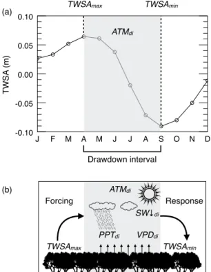
Our globally applicable approach used the annual cycle of TWS drawdown and recharge to isolate the months of the year during which the land surface loses moisture, which we refer to as the drawdown interval (Fig. 1a). We selected this interval because past work has shown that the land sur-face’s influence on the atmosphere is most prevalent during summer in the Northern Hemisphere (Cheruy et al., 2014; Phillips and Klein, 2014) and during the dry season in trop-ical forests (Harper et al., 2013; Lorenz and Pitman, 2014). This approach allowed us to investigate land surface coupling at a global scale, and to extend metrics developed in previ-ous work for pre-defined monthly intervals corresponding to boreal summer (e.g., Guo and Dirmeyer, 2013; Koster et al., 2006) to be applicable to any seasonality.
J F M A M J J A S O N D -0.10
-0.05 0.00 0.05 0.10
T
W
SA
(m)
TWSAmax
Drawdown interval
TWSAmin
ATMdi
ATMdi
TWSAmax TWSAmin
Forcing Response
PPTdi
SW↓di
VPDdi
(a)
(b)
Figure 1. Conceptual description of coupling metrics:(a) exam-ple TWSA climatology from a typical midlatitude location in cen-tral North America (38◦N, 92◦W) illustrating the definition of
the drawdown interval as the months from the maximum TWSA through the minimum TWSA. TWSAmaxand TWSAmin are the TWSA values (in units of water height) during the maximum and minimum months, respectively, and ATMdiis the atmospheric vari-able of interest averaged across the months of the drawdown in-terval.(b)Representation of the interactions between TWS and at-mospheric component, demonstrating the forcing limb of the feed-back loop, in which TWSAmaxforces subsequent atmospheric con-ditions, as well as the response limb, in which TWSAminresponds to the atmospheric state during the drawdown interval.
2 Methods
2.1 Remote sensing data
We obtained level 3 TWSA data from GRACE using the Uni-versity of Texas at Austin Center for Space Research (CSR) spherical harmonic solutions (Swenson, 2012). Global land data at a 1◦resolution were scaled using the coefficients
pro-vided by Landerer and Swenson (2012). The study period was limited to September 2002 through November 2014, in order to minimize temporal gaps. GRACE data during the study period included 8 non-consecutive and 2 consecutive missing months, which were filled using linear interpolation. At each grid cell, the TWSA time series was decomposed into linear trend, seasonal cycle, and interannual variability components using ordinary least squares regression. This de-composition allowed us to estimate a mean annual cycle at each grid cell with minimal influence of any long-term trend.
Level 3 near-surface temperature and relative humidity were obtained globally at a monthly, 1◦ resolution from
the ascending (daytime) orbit of the Atmospheric Infrared Sounder (AIRS) platform (Susskind et al., 2014). Vapor pres-sure deficit (VPD) was calculated from the AIRS data using the August–Roche–Magnus approximation to the Clausius– Clapeyron relation (Lawrence, 2005). Precipitation (PPT) data were obtained from the Global Precipitation Clima-tology Project (GPCP), a merged satellite and gauge-based data set (Huffman et al., 2009), at a daily, 1◦ resolution
and then integrated monthly. Downwelling shortwave radi-ation (SW↓) was obtained globally at a monthly, 1◦
resolu-tion from the Clouds and the Earth’s Radiant Energy Sys-tem (CERES) Energy Balanced and Filled (EBAF) surface product (Loeb et al., 2009). More information describing the remote sensing and reanalysis data products used in our anal-ysis is summarized in Table 1.
2.2 Drawdown interval
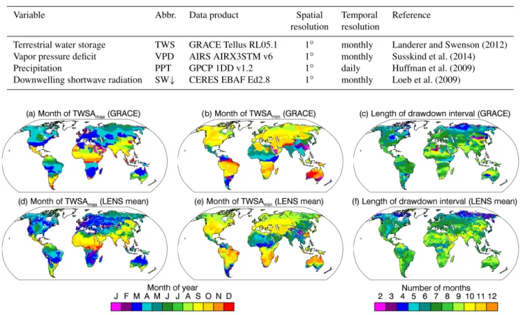
As a first step, we used the mean annual cycle from GRACE to determine the months of the maximum and minimum TWS anomalies in order to define the drawdown interval at each 1◦ land grid cell (Fig. 2). Northern Hemisphere
mid-dle and high latitudes exhibited a drawdown interval begin-ning in the spring (MAM, March–April–May) and ending in the late summer or fall (ASO, August–September–October), reflecting the timing of the boreal summer growing season. At lower latitudes, the North American, African, and Asian monsoons were evident, with Mexico, India, and the Sahel showing a drawdown interval beginning in September, after the monsoonal precipitation has peaked, and ending the fol-lowing spring after the winter dry season. The onset of the drawdown interval reversed abruptly at the Equator in Africa and Asia, with the drawdown interval reflecting a winter dry season in the austral low latitudes transitioning to a sum-mer growing season in the austral midlatitudes. Within the months of our study period, the portion of land grid cells that experience 11, 12, and 13 complete drawdown intervals are 9.4, 90.5, and 0.1 %, respectively.
2.3 Coupling metrics
Table 1.Remote sensing products used for analysis.
Variable Abbr. Data product Spatial Temporal Reference resolution resolution
Terrestrial water storage TWS GRACE Tellus RL05.1 1◦ monthly Landerer and Swenson (2012) Vapor pressure deficit VPD AIRS AIRX3STM v6 1◦ monthly Susskind et al. (2014) Precipitation PPT GPCP 1DD v1.2 1◦ daily Huffman et al. (2009)
Downwelling shortwave radiation SW↓ CERES EBAF Ed2.8 1◦ monthly Loeb et al. (2009)
Figure 2.Month of maximum and minimum TWSA and the length of the drawdown interval from GRACE(a–c)and the LENS ensemble mean(d–f). Months of maximum and minimum were based on the climatology of detrended TWSA over the 146 months in the GRACE record.
We defined our forcing metric as the Pearson product-moment correlation coefficient between the TWS anomaly at the onset of the drawdown interval (TWSAmax) and the surface atmospheric conditions during the drawdown inter-val (abbreviated here as ATMdi). In our analysis, we se-lected three variables to represent the atmospheric state: VPD, SW↓, and PPT. These atmospheric variables were av-eraged during the drawdown interval, including during the months of climatological maximum and minimum TWSA. We chose these variables because they represent various as-pects of evaporative supply (PPT) and demand (VPD and SW↓).
Similarly, we defined our response metric as the correla-tion coefficient between ATMdiand the land surface state at the end of the drawdown interval (TWSAmin). Although most previous diagnoses of land–atmosphere coupling has focused on the forcing limb, we argue the response limb is equally important as a metric for model evaluation. Specifically, if variability in the balance between evaporative supply and de-mand does not lead to the correct TWS variability, then the incorrect TWS response will feed back into subsequent forc-ing on the atmosphere.
We note that these metrics do not provide distinctive infor-mation for measuring the strength of land–atmosphere cou-pling or the land surface response. While the metrics include the influence of direct land–atmosphere interactions, they are also potentially influenced by atmospheric and soil moisture persistence, as well as remote forcing from sea surface tem-peratures (SSTs) (Orlowsky and Seneviratne, 2010; Mei and Wang, 2011). Nevertheless, these metrics may still serve as useful benchmarks against which to evaluate the ability of ESMs to reproduce the proper relationships based on the combination of these factors.
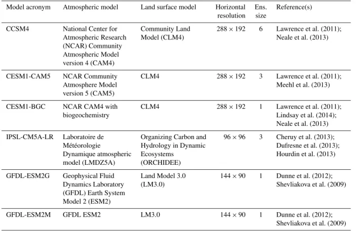
sur-Table 2.CMIP5 models used for analysis.
Model acronym Atmospheric model Land surface model Horizontal Ens. Reference(s) resolution size
CCSM4 National Center for Community Land 288×192 6 Lawrence et al. (2011); Atmospheric Research Model (CLM4) Neale et al. (2013) (NCAR) Community
Atmospheric Model version 4 (CAM4)
CESM1-CAM5 NCAR Community CLM4 288×192 3 Lawrence et al. (2011);
Atmosphere Model Meehl et al. (2013)
version 5 (CAM5)
CESM1-BGC NCAR CAM4 with CLM4 288×192 1 Lawrence et al. (2011); biogeochemistry Lindsay et al. (2014);
Neale et al. (2013)
IPSL-CM5A-LR Laboratoire de Organizing Carbon and 96×96 3 Cheruy et al. (2013); Météorologie Hydrology in Dynamic Dufresne et al. (2013); Dynamique atmospheric Ecosystems Hourdin et al. (2013) model (LMDZ5A) (ORCHIDEE)
GFDL-ESM2G Geophysical Fluid Land Model 3.0 144×90 1 Dunne et al. (2012); Dynamics Laboratory (LM3.0) Shevliakova et al. (2009) (GFDL) Earth System
Model 2 (ESM2)
GFDL-ESM2M GFDL ESM2 LM3.0 144×90 1 Dunne et al. (2012); Shevliakova et al. (2009)
face to VPD would also be associated with a negative corre-lation coefficient.
Because the partitioning of surface fluxes can, depending on the spatiotemporal scale, cause a change of either sign to cloudiness and precipitation (Taylor et al., 2012; Guillod et al., 2015), correlation coefficients of either sign could indi-cate strong land surface forcing on PPT and SW↓. However, the response metrics would be expected to show greater con-sistency. Higher PPT during the drawdown interval would be expected to increase TWS (positive correlation), while higher SW↓would increase evaporative demand, thereby de-creasing TWS (negative correlation). Therefore, to maintain consistent nomenclature based on evaluating the strength of a positive moisture feedback, we consider strong coupling in both the forcing and response metrics to be associated with a positive correlation in the case of PPT and a negative corre-lation in the case of SW↓.
2.4 Community Earth System Model Large Ensemble We used the metrics described above to evaluate feedback strength in the CESM LENS. LENS comprises an ensem-ble of 38 fully coupled runs in which air temperature ini-tial conditions are perturbed slightly (by an amount less than the round-off error) to reveal the internal variability inherent within the coupled climate model. LENS has demonstrated that the uncertainty in climate projections due to internal
climate variability inherent in CESM is comparable to the ranges of output within the entire CMIP5 experiment (Kay et al., 2014). LENS uses version 1 of CESM (CESM1) with version 5 of the Community Atmosphere Model (CAM5) and version 4 of the Community Land Model (CLM4) at a hori-zontal resolution of 1◦. The ensemble run follows protocols
from the CMIP5 experiment, with historical radiative forcing for the 20th century and representative concentration path-way 8.5 (RCP8.5) forcing for the 21st century.
The LENS data were chosen as a starting point for feed-back evaluation for two reasons. First, the availability of a TWS variable in these simulations enabled a direct compari-son with metrics derived using data from GRACE. The TWS field in CLM4 included water from surface and canopy stor-age, snow and ice, soil moisture, and a dynamic aquifer, in addition to river water storage terms from the coupled River Transport Module (RTM). The coupling of CLM4 with RTM has been shown to be important for simulating both the an-nual cycle and interanan-nual variability of TWS in comparison with GRACE (Kim et al., 2009).
decadal-scale variability (Kay et al., 2014). Analyzing the full ensemble from LENS enabled us to assess the sensitivity of our forcing and response metrics to this variability. We ex-tracted from each ensemble member the equivalent months of the satellite record, with data prior to December 2005 coming from the historical runs, and data from January 2006 onward coming from the RCP8.5 simulations.
2.5 Assessment of uncertainty
To assess the sensitivity of our metrics to observational un-certainty, we used a Monte Carlo sampling approach. For each of the 38 members of LENS, we calculated coupling metrics 10 times with random noise added to both TWSA and atmospheric variable time series at each grid cell. The noise was randomly generated from a Gaussian distribution with a mean of zero and a standard deviation equal to 25 % of the standard deviation of the original data. Comparing these results with those from the unaltered data provided some in-dication of how much our coupling metrics are degraded by random noise as an approximation of observational uncer-tainty.
In addition, to assess how our analysis may be influenced by uncertainty due to the selection of satellite data, we sub-stituted data from the European Centre For Medium-range Weather Forecasting (ECMWF) Interim Reanalysis (ERA-Interim) (Dee et al., 2011) in place of AIRS-, GPCP-, and CERES-derived variables. We only used atmospheric reanal-ysis data for this sensitivity analreanal-ysis, as these data benefit from assimilation of observations, while we continued to use GRACE for TWSA. Comparing results from this GRACE-reanalysis hybrid to those using only satellite data provided a general indication of how sensitive our coupling metrics were to the data source.
2.6 CMIP5 analysis
To extend our analysis to models that did not output an ex-plicit TWS field, we compared accumulated residuals of pre-cipitation, evapotranspiration, and total runoff (surface and subsurface) with the explicit TWS variable in the LENS simulations. We also compared coupling metrics calculated from LENS using accumulated residuals with those calcu-lated from the explicit TWS field. After we determined that the accumulated residuals of the water balance represented much of the variability in the explicit TWS variable and yielded coupling metrics with similar distributions within LENS, we calculated equivalent metrics for several model simulations in the CMIP5 archive (Table 2). We selected the CMIP5 models that were similar to LENS (CESM1-CAM5 and CESM1-BGC) as well as the models that participated in the GLACE-CMIP5 experiment (Seneviratne et al., 2013) for which each necessary output field was available (CCSM4, GFDL-ESM2M, GFDL-ESM2G and IPSL-CM5A-LR).
3 Results
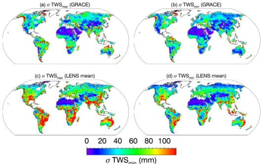
3.1 Drawdown interval and interannual variability A comparison of the months of maximum and minimum terrestrial water storage as determined by climatologies of GRACE and the LENS ensemble mean indicated that the model largely reproduces the timing of TWSA seasonality evident in the satellite observations (Fig. 2). Geographic pat-terns of seasonality were consistent between the model and observations, though a phase shift in the drawdown interval is apparent in eastern Canada and central Eurasia where LENS had a 1-month early bias for both the maximum and min-imum TWSA, in southeast North America where the onset of the modeled drawdown interval was slightly later than the observations, and in parts of east Asia and Australia where the modeled drawdown interval ended earlier than in the observations. However, despite capturing generally correct timing, the model exhibited higher interannual variability of TWSAmaxand TWSAminacross the 11–12 drawdown inter-vals compared with the satellite data (Fig. 3) particularly in the southern United States, southern South America, central and eastern Africa, southern Asia, and eastern Australia. One possible explanation for this is the presence of multi-year trends in aquifer storage in CLM4 that are not consistent with GRACE (Swenson and Lawrence, 2015).
A comparison of the interannual variability of atmospheric variables across multiple drawdown intervals between the model and satellite data showed various degrees of con-sistency (Fig. 4). The magnitude and geographic pattern of VPDdi was generally consistent, though LENS showed greater interannual variability than AIRS in central and west-ern North America, South America, northwest-ern and south-ern Africa, and southsouth-ern Asia. In the case of PPTdi, LENS showed less interannual variability than GPCP in southeast North America and much of South America, but the two were largely consistent elsewhere. SW↓diwas the least con-sistent between the model and satellite data, as LENS showed greater interannual variability than CERES in southern North America, northern Eurasia, most of Africa, and most of Aus-tralasia.
Figure 3.Interannual variability (standard deviation) of TWSAmaxand TWSAminfrom GRACE(a, b)and the LENS ensemble mean(c, d).
Figure 4.Interannual variability (standard deviation) of VPDdifrom AIRS(a), PPTdifrom GPCP(b), SW↓difrom CERES(c)and the equivalent quantities from the LENS ensemble mean(d–f).
3.2 Evaluating feedbacks for a single model simulation
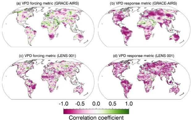
The forcing metric for VPD derived from GRACE and AIRS showed regions of strong coupling, in which TWSAmax was negatively correlated with VPDdi, in the northern Great Plains, northern South America, southern Africa, south-ern and westsouth-ern India, north central Eurasia, and northsouth-ern Australia (Fig. 5a). Regions with strong positive correla-tion were much less common, and were largely confined to areas of very low GRACE-derived TWSAmax variability (Fig. 3a). Positive correlations are unlikely to reflect direct land–atmosphere coupling. Instead, they demonstrate how
remote SST forcing, depending on persistence and time de-lays with atmospheric responses, can lead to apparent neg-ative relationships such as those demonstrated by Wei et al. (2008). In comparison with the satellite data, the VPD forcing metrics from the first ensemble member of LENS (Fig. 5c) showed much stronger coupling in the southern and eastern Amazon, and marginally stronger coupling strength across many regions in temperate Asia.
correla-Figure 5.Forcing and response metrics for VPD from GRACE/AIRS(a, b)and LENS ensemble member 001(c, d). Cross-hatching indicates a correlation coefficient that is statistically significant atp≤0.05.
tions found only in arid regions of low TWS variability. Par-ticularly strong response metrics were found in eastern North America, northern South America, western Eurasia, the Sa-hel, India, and eastern Australia. The first ensemble mem-ber from LENS showed widespread negative correlations, and did not show the positive correlations found in the satel-lite data. Response coupling in LENS was much more spa-tially homogeneous than in the satellite data, though north-ern South America and westnorth-ern Eurasia still showed stronger coupling than elsewhere.
Many of the areas that showed a strong forcing metric for VPD also showed a relatively strong forcing metric for PPT, though the PPT forcing metric was overall weaker than that for VPD (Fig. 6a). The response metric for PPT was gener-ally positive, indicating that for much of the globe, a more positive TWSAmin was associated with higher precipitation rates (Fig. 6b). Both the forcing and response metrics were somewhat stronger in the LENS member relative to those ev-ident in the satellite data (Fig. 6c and d).
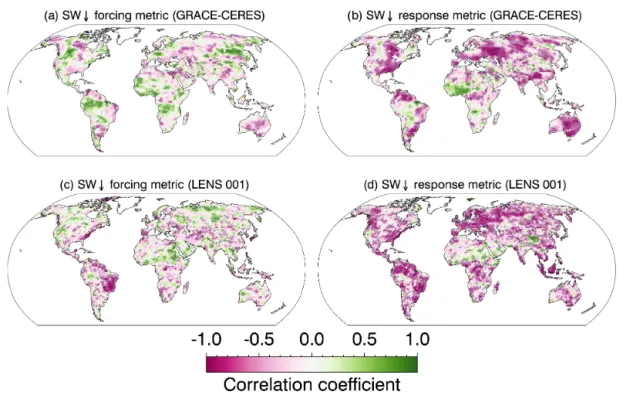
The forcing metrics for SW↓showed a mixture of positive and negative correlations, indicating that higher TWSAmax was either positively or negatively coupled with shortwave radiation (Fig. 7a). This finding is consistent with both posi-tive and negaposi-tive coupling between cloud cover and terres-trial moisture observed over shorter timescales (Taylor et al., 2012; Guillod et al., 2015). The response metrics for SW↓ were generally negative, indicating that greater sea-sonal shortwave radiation was associated with more nega-tive TWSAmin (stronger coupling), with western Africa
be-ing a notable exception (Fig. 7b). The LENS member showed generally stronger coupling in both the forcing and response metrics for SW↓(Fig. 7c and d).
3.3 Evaluating the CESM Large Ensemble
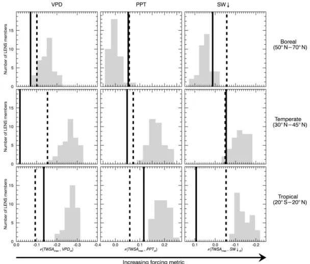
In temperate and tropical regions, forcing metrics were gen-erally stronger in LENS (more positive correlations for PPT, more negative for VPD and SW↓) than in the satellite and reanalysis data, indicating a stronger land surface forcing of the surface atmospheric state in the model than in the obser-vations (Fig. 8). In boreal regions, forcing metrics were much weaker (closer to zero) than at lower latitudes in both the satellite data and in LENS, indicating very little relationship between TWSAmaxand ATMdi. This is consistent with high levels of climate variability in many high-latitude regions driven by the Arctic Oscillation, the North Atlantic Oscilla-tion, and other dynamical modes (Cohen and Barlow, 2005). Furthermore, at high latitudes, ET is generally energy lim-ited rather than moisture limlim-ited, which would lead to weak forcing metrics as moisture availability would not strongly influence atmospheric conditions.
differ-Figure 6.Forcing and response metrics for PPT from GRACE/GPCP(a, b)and LENS ensemble member 001(c, d). Cross-hatching indicates a correlation coefficient that is statistically significant atp≤0.05.
Figure 7.Forcing and response metrics for SW↓ from GRACE/CERES(a, b)and LENS ensemble member 001(c, d). Cross-hatching indicates a correlation coefficient that is statistically significant atp≤0.05.
ence between metrics as measured by the satellite data com-pared with the reanalysis data, the general pattern indicated that modeled response metrics were higher than those from observations and reanalysis.
3.4 Analysis of uncertainty
met-Figure 8.Ensemble histogram of forcing metrics from the 38 simulations in LENS (gray bars) compared to satellite observations from GRACE/AIRS/GPCP/CERES (solid black line) and the alternate set of observations from GRACE and ERA-Interim (dashed black line), averaged across land regions within different latitude bands.
rics with a spread on the same order of magnitude as the difference between modeled and satellite-derived zonal av-erages. The distribution of coupling metrics from LENS re-vealed the sensitivity of the relationships to decadal climate variability given the relatively short TWS time series. Com-paring this distribution with the spread between the purely satellite-derived metrics and GRACE-reanalysis hybrid in-dicated the sensitivity of our metrics to the choice of data source. The differences between satellite and reanalysis met-rics were generally greater in the tropics, particularly for VPD and SW↓, and in midlatitude VPD for both forcing and response variables. Elsewhere, the differences were generally similar to or less than the differences between the observa-tionally constrained zonal averages and the LENS distribu-tions.
Comparing the original LENS forcing and response met-rics with those calculated after adding random noise to LENS (Figs. S1 and S2 in the Supplement) provided an estimate of the metrics’ sensitivity to observational uncertainty. Adding random noise with 25 % of the standard deviation of the
orig-inal data to the model time series of TWSA and atmospheric variables at each grid cell does degrade the metrics slightly, causing areal averages to be closer to zero, but the differences are relatively small compared to the differences between ob-served and modeled averages as well as the spread of the ensemble itself. This sensitivity analysis provided evidence that observational errors likely have a relatively small impact on the quality of our satellite-derived metrics.
3.5 Evaluating CMIP5 models
Figure 9.Ensemble histogram of response metrics from the 38 simulation in LENS (gray bars) compared to satellite observations from GRACE/AIRS/GPCP/CERES (solid black line) and the alternate set of observations from GRACE and ERA-Interim (dashed black line), averaged across land regions within different latitude bands.
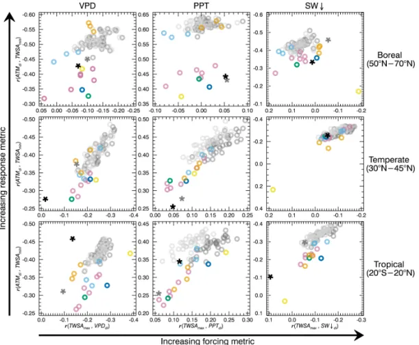
for PPT was apparent in the middle and low latitudes, but the remaining metrics are not highly sensitive to TWS formula-tion. This suggests that metrics calculated for CMIP5 output using accumulated residuals could be reasonably and effec-tively compared with the metrics derived from LENS and the observations (Fig. 10).
As with LENS, the metrics derived from CMIP5 output in-dicated generally stronger coupling metrics than the observa-tions for both the forcing and response limbs. Excepobserva-tions in-clude the VPD response metric in the tropics, the boreal PPT and SW↓forcing metrics, and the midlatitude SW↓response metrics. The spread between various models was generally greater than the spread within any single model with a multi-member ensemble. Of the four models that use CLM4 for the land surface, the two that use CAM5 for the atmosphere (LENS and CESM1-CAM5) were clustered close together, and exhibited generally the strongest forcing and response metrics. The two that use CAM4 (CCSM4 and CESM1-BGC) were close to each other, but with lower metrics in both forcing and response than the CAM5 models. The two
GFDL models were both within the general ensemble range in the metrics for both VPD and PPT, but GFDL-ESM2M was an extreme outlier in both forcing and response metrics for SW↓.
4 Discussion
4.1 Benchmarking models with observed coupling metrics
The metrics developed here from satellite observations pro-vide a means for evaluating land–atmosphere feedback strength on seasonal to interannual timescales in coupled ESMs. The use of correlation coefficients in this study does not enable a direct assessment of whether the rela-tionships are directly causal, as correlation between spheric and terrestrial conditions could result from atmo-spheric persistence and remote forcing from SSTs (Orlowsky and Seneviratne, 2010; Mei and Wang, 2011). Nonetheless, the satellite-derived metrics provide a meaningful constraint against which coupled models can be benchmarked, as these models need to correctly represent the combined effects of persistence, remote SST forcing, and land–atmosphere cou-pling.
The forcing metrics, by indicating the relationship be-tween antecedent TWS and subsequent atmospheric char-acteristics, provide observational constraints to complement previous research in large-scale land–atmosphere coupling in global models (e.g., Guo and Dirmeyer, 2013; Koster et al., 2006; Seneviratne et al., 2013). Observed forcing metrics were found to be strong in some of the regions of interme-diate wetness in which ET is limited by terrestrial moisture availability, in addition to some regions in the moist trop-ics in which ET is generally considered to be energy lim-ited. Recent observational analyses by Hilker et al. (2014) demonstrated that at least in the Amazon, deep rooting-zone water supplies can become seasonally depleted, leading to a stronger land–atmosphere coupling. This is consistent with findings that deep rooted plants vertically redistribute soil water to shallower layers, allowing higher levels of evapo-transpiration to be sustained during the dry season (Lee et al., 2005). It is also consistent with recent work demonstrating that TWSAs can be used as predictors for fire season sever-ity in the Amazon (Chen et al., 2013).
The inclusion of response metrics in our analysis allows the full feedback loop to be considered by recognizing the two-way dependence between the land surface and the atmo-sphere. The generally higher correlation coefficients in ob-served response metrics indicates the importance of the land surface response in priming the system for subsequent forc-ing on the atmosphere. For example, if the TWS response is too strongly coupled to the atmosphere, a small change in atmospheric conditions could yield an unrealistically large change in TWS. The unrealistically large TWS anomaly, in turn, would have the potential to impart a larger land sur-face forcing of the atmosphere in subsequent time steps. That models and ensemble members with high forcing met-rics were also generally found to have high response metmet-rics (Fig. 10) highlights the need to consider this.
Both the forcing and response metrics as calculated from the output of the ESMs analyzed in the current study indi-cated generally stronger coupling compared with those de-rived from the satellite observations. There are exceptions to this pattern, but it holds generally true, particularly across middle and lower latitudes, and particularly in the LENS data. This is consistent with previous studies conducted at finer temporal resolutions (Ferguson et al., 2012) and across more limited spatial domains (Hirschi et al., 2011). As de-scribed below, there are several possible explanations as to why models may simulate a stronger feedback than is ob-served in the satellite record.
4.2 Possible explanations for enhanced feedback strength in models
One set of possible explanations for the stronger coupling metrics in models relative to observations involves models overestimating the amount of water available for ET dur-ing the drawdown interval. The land surface influence on the atmosphere requires water to be a limiting factor to ET but not limiting enough to prevent it altogether. Under more moisture-limited conditions, a drawdown interval may expe-rience multiple shorter time periods during which ET is in-hibited due to insufficient water, and the terrestrial moisture state exerts no control over flux partitioning. These periods of insufficient moisture would tend to reduce the overall feed-back strength integrated across the duration of the drawdown interval. Model shortcomings that make water too readily available for ET could reduce the amount of time spent in a periods of insufficient moisture during the drawdown in-terval, thereby unrealistically strengthening the longer-term feedback. We note that the opposite could take place un-der near-saturated conditions if a model overestimates the amount of time in which ET is energy limited, but we would not expect these conditions to be as prevalent during the drawdown interval that was the time period of focus in our analysis.
param-Figure 10.Scatter plots of forcing and response metrics for LENS and CMIP5 models with observations, averaged across land regions within different latitude bands. For LENS, we show metrics calculated using the explicit TWS output (darker gray) and TWSA estimates from the accumulated residuals of the surface water balance (lighter gray). For CMIP5 models, we calculated metrics using TWSA estimates from the accumulated residuals of the surface water balance.
eterization is replaced with embedded cloud-resolving mod-els (Kooperman et al., 2016).
A misrepresentation of either the amount of bare soil or of bare soil processes also could lead to overestimates of the amount of water available for ET and thereby coupling strength. Current land surface schemes of ESMs are based on the “big leaf” model paradigm, which could lead to overesti-mates of ET if runoff and groundwater recharge are underes-timated as a consequence of an unrealistically small bare soil fraction. In addition, even if bare soil fraction were correct, overestimates of ET due to an incomplete representation of surface resistance of bare soil, as found in CLM4 by Swen-son and Lawrence (2014), would amplify positive feedbacks. Additional explanations for why models may overestimate feedback strength include the parameterization of convection in the PBL or stomatal conductance responses to soil mois-ture. Previous work using a regional climate model (RCM) with a higher spatial resolution have determined that convec-tive parameterizations are as important as spatial resolution in the simulation of precipitation coupling (Hohenegger et
al., 2009). Taylor et al. (2013) similarly found parameter-ized convection in an RCM yielding a positive coupling in contrast to the negative coupling found in both observations and model runs with explicitly simulated convection. If neg-ative coupling mechanisms are present in reality but absent from models, this could contribute to an overestimate of cou-pling metrics and underrepresentation of negative feedbacks in models. Similarly, the diversity of stomatal conductance parameterizations in CMIP5 ESMs is relatively low (Medlyn et al., 2011; Swann et al., 2016), and if stomatal apertures close too rapidly in response to an initial deficit in terrestrial water storage, transpiration–humidity feedbacks may be in-tensified in an unrealistic manner.
land–atmosphere coupling (Findell et al., 2015). Given the relatively short time series available for the current analy-sis, the correlation coefficients derived from remote sensing data may be reduced due to observational uncertainty, unlike those derived from internally consistent models. We found that adding random noise to LENS at 25 % of the standard deviation of the original data caused some degradation of our area-averaged coupling metrics, but only by a small amount relative to the difference between LENS and the observa-tions (Figs. S1 and S2). We chose 25 % as a qualitative upper bound on likely uncertainties introduced from random ob-servational error within the TWSA and atmospheric variable time series. This highlights the need for developing more quantitative error estimates in remote sensing and reanalysis products. More generally, this sensitivity analysis suggests that our coupling metrics, when averaged across large areas, may be useful in identifying robust data–model differences.
Another possible explanation stems from the fact that our coupling metrics include co-variability due to atmo-spheric persistence and remote forcing by SST (Orlowsky and Seneviratne, 2010; Mei and Wang, 2011) alongside the direct influence of land–atmosphere interactions. For this reason, we caution that overestimates of coupling metrics do not imply that the land–atmosphere feedback is neces-sarily stronger, but could be due to an overestimate of SST-driven correlations between the land surface and the atmo-sphere. Wei et al. (2008) demonstrated that negative cor-relations between soil moisture and subsequent precipita-tion can be explained by precipitaprecipita-tion persistence combined with negative temporal autocorrelation of precipitation asso-ciated with intra-seasonal modes such as the Madden–Julian Oscillation (MJO). Poor representation of the MJO period in CMIP5 models leads to unrealistic patterns of precipita-tion persistence (Hung et al, 2013). If models are failing to capture MJO-driven negative correlations, this could lead to overly strong positive correlations relative to observations. However, this would depend on the length of the drawdown interval relative to persistence time and the period of intra-seasonal modes.
4.3 Uncertainties and future applications
The current study demonstrates the utility of the coupling metrics presented here, but conclusions are limited by the time span of the satellite record. While LENS enables the internal variability of these relationships to be investigated within the model, it is unclear how much natural climate variability affects these relationships in reality on timescales longer than the satellite record. Furthermore, we acknowl-edge that observational error over an insufficiently long time series could reduce the apparent strength of correlations (Findell et al., 2015). Therefore, the utility of the coupling metrics we present will increase alongside the length of the time series available from remote sensing platforms. This emphasizes the importance of the GRACE follow-on
mis-sion (Flechtner et al., 2014) and the need for continuity in the record between missions.
Furthermore, incorporating additional remote sensing products can reduce uncertainties inherent in the satellite-derived data sets. We presented metrics satellite-derived using ERA-Interim in place of AIRS, GPCP, and CERES in order to qualitatively illustrate this uncertainty. We found a non-negligible amount of uncertainty in both forcing and re-sponse metrics due to inconsistencies between the remote sensing and reanalysis products. Future work will address these uncertainties by incorporating additional observations and observationally constrained data sets such as those from the Global Soil Wetness Project (Dirmeyer et al., 2006b) and the Global Land Data Assimilation System (Rodell et al., 2004). In addition, as increasingly long time series of data become available from the Soil Moisture Ocean Salinity (Mecklenburg et al., 2012) and Soil Moisture Active Passive (Panciera et al., 2014) missions, the metrics developed here can be applied to those data sets as well, which will elucidate the importance of surface soil moisture relative to the total TWS column in these interactions.
Finally, the issue of causality and the possibility that cor-relations result primarily from atmospheric persistence and remote forcing from SST rather than land–atmosphere inter-actions may be addressed using sensitivity experiments sim-ilar to those of the GLACE and GLACE-CMIP experiments. While the previous experiments have tested the importance of soil moisture interaction with the atmosphere, additional experiments could expand upon these methods by treating SST variability similar to terrestrial soil moisture availability. Such experiments could determine the relative importance of remote SST forcing, including the effect of atmospheric per-sistence, and local land–atmosphere coupling in explaining correlations between TWS and atmospheric conditions.
As these sources of uncertainty are diminished, the cou-pling metrics introduced here may be used to assess whether improvements to model biogeophysics and parameteriza-tions yield relaparameteriza-tionships that are more consistent with obser-vations. CMIP5 models are known to have a high ET bias (Mueller and Seneviratne, 2014), which could be due in part to the explanations proposed as possible reasons for overes-timated coupling metrics in models. As data become avail-able from phase 6 of the Coupled Model Intercomparison Project (CMIP6), these metrics could provide an assessment of whether improvements to ET processes in models also im-proves the relationship between the land surface and the at-mosphere.
5 Conclusion
GRACE mission, along with concurrently collected remote sensing and reanalysis data sets of atmospheric variables, in a manner that could then be applied to Earth system models. The coupling metrics described here quantify the relation-ships between both antecedent TWS and subsequent atmo-spheric conditions, as well as antecedent atmoatmo-spheric condi-tions and subsequent TWS.
Regions of strong forcing, in which the TWSA at the be-ginning of the drawdown interval was related to the subse-quent atmospheric state, coincided with the semi-arid zones previously found to be hot spots of land–atmosphere cou-pling, as well as some new tropical zones that may have moisture-limited ET regimes. Regions of strong response metrics, in which the TWSA at the end of the draw-down interval is related to the atmosphere, are much more widespread. Modeled coupling metrics are generally found to be stronger than those observed in the satellite record. If this discrepancy is due to models overestimating the two-way feedback between the land surface and the atmosphere, this could lead to models incorrectly projecting future warm-ing trends and climatic extremes (e.g., Hirschi et al., 2011; Seneviratne et al., 2013; Cheruy et al., 2014; Miralles et al., 2014).
The results of this study are consistent with previous stud-ies at smaller temporal scales indicating land–atmosphere coupling strength may be stronger in models than in observa-tions. There are several possible mechanisms that may con-tribute to the overestimation of land–atmosphere coupling in models, and future studies may incorporate the metrics in-troduced here to assess the role of these mechanisms. These metrics will become increasingly useful as the temporal cov-erage of the remote sensing record grows longer and addi-tional missions come online.
6 Data availability
All data used in this analysis are publicly available. GRACE Monthly Land Water Mass Grids NetCDF Re-lease 5.0 is available from http://podaac.jpl.nasa.gov/dataset/ TELLUS_LAND_NC_RL05, doi:10.5067/TELND-NC005. AIRS/Aqua L3 Monthly Standard Physical Retrieval (AIRX3STM) v0006 is available from http://disc.sci. gsfc.nasa.gov/uui/datasets/AIRX3STM_V006/summary, doi:10.5067/AQUA/AIRS/DATA319. GPCP One-Degree Daily v1.2 is available from http://precip.gsfc.nasa.gov. CERES EBAF-Surface is available from https: //ceres.larc.nasa.gov/products.php?product=EBAF-Surface. ERA-Interim is available from http://www.ecmwf.int/ en/research/climate-reanalysis/era-interim. CESM LENS is available from http://www.cesm.ucar.edu/projects/ community-projects/LENS/data-sets.html. CMIP5 archives are available through the Earth System Grid Federation at http://pcmdi9.llnl.gov/.
The Supplement related to this article is available online at doi:10.5194/hess-20-4837-2016-supplement.
Acknowledgements. We received funding support from the United States Department of Energy Office of Science Biogeochemistry Feedbacks Scientific Focus Area and the Climate Change Prediction Program, cooperative agreement (DE-FC03-97ER62402/A010). The CESM Large Ensemble Community Project was supported by the National Science Foundation (NSF) with supercomputing re-sources provided by the Climate Simulation Laboratory at NCAR’s Computational and Information Systems Laboratory (CISL). We also acknowledge the World Climate Research Programme’s Work-ing Group on Coupled ModellWork-ing, which is responsible for CMIP, and we thank the climate modeling groups (listed in Table 2 of this paper) for producing and making available their model output. For CMIP, the US Department of Energy’s Program for Climate Model Diagnosis and Intercomparison provides coordinating support and led the development of software infrastructure in partnership with the Global Organization for Earth System Science Portals.
Edited by: P. Gentine
Reviewed by: T. Ford and two anonymous referees
References
Alfieri, L., Claps, P., D’Odorico, P., Laio, F., and Over, T. M.: An analysis of the soil moisture feedback on convective and stratiform precipitation, J. Hydrometeorol., 9, 280–291, doi:10.1175/2007JHM863.1, 2008.
Berg, A., Lintner, B. R., Findell, K., Seneviratne, S. I., van den Hurk, B., Ducharne, A., Chéruy, F., Hagemann, S., Lawrence, D. M., Malyshev, S., Meier, A., and Gentine, P.: Interannual Coupling between Summertime Surface Temperature and Pre-cipitation over Land: Processes and Implications for Climate Change, J. Climate, 28, 1308–1328, doi:10.1175/JCLI-D-14-00324.1, 2015.
Betts, A. K.: Land-surface–atmosphere coupling in observa-tions and models, J. Adv. Model. Earth Syst., 1, 4, doi:10.3894/JAMES.2009.1.4, 2009.
Betts, A. K., Desjardins, R., Worth, D., and Beckage, B.: Cli-mate coupling between temperature, humidity, precipitation, and cloud cover over the Canadian Prairies, J. Geophys. Res.-Atmos., 119, 13305–13326, doi:10.1002/2014JD022511, 2014.
Chen, Y., Velicogna, I., Famiglietti, J. S., and Randerson, J. T.: Satellite observations of terrestrial water storage provide early warning information about drought and fire season sever-ity in the Amazon, J. Geophys. Res.-Biogeo., 118, 495–504, doi:10.1002/jgrg.20046, 2013.
Chen, Y., Morton, D. C., Andela, N., Giglio, L., and Randerson, J. T.: How much global burned area can be forecast on seasonal time scales using sea surface temperatures?, Environ. Res. Lett., 11, 45001, doi:10.1088/1748-9326/11/4/045001, 2016. Cheruy, F., Campoy, A., Dupont, J.-C., Ducharne, A., Hourdin, F.,
Cheruy, F., Dufresne, J. L., Hourdin, F., and Ducharne, A.: Role of clouds and land–atmosphere coupling in midlatitude conti-nental summer warm biases and climate change amplification in CMIP5 simulations, Geophys. Res. Lett., 41, 6493–6500, doi:10.1002/2014GL061145, 2014.
Cohen, J. and Barlow, M.: The NAO, the AO, and global warming: how closely related?, J. Climate, 18, 4498–4513, doi:10.1175/JCLI3530.1, 2005.
Dai, A.: Precipitation characteristics in eighteen coupled climate models, J. Climate, 19, 4605–4630, doi:10.1175/JCLI3884.1, 2006.
Dee, D. P., Uppala, S. M., Simmons, A. J., Berrisford, P., Poli, P., Kobayashi, S., Andrae, U., Balmaseda, M. A., Balsamo, G., Bauer, P., Bechtold, P., Beljaars, A. C. M., van de Berg, L., Bid-lot, J., Bormann, N., Delsol, C., Dragani, R., Fuentes, M., Geer, A. J., Haimberger, L., Healy, S. B., Hersbach, H., Hólm, E. V., Isaksen, L., Kållberg, P., Köhler, M., Matricardi, M., McNally, A. P., Monge-Sanz, B. M., Morcrette, J.-J., Park, B.-K., Peubey, C., de Rosnay, P., Tavolato, C., Thépaut, J.-N., and Vitart, F.: The ERA-Interim reanalysis: configuration and performance of the data assimilation system, Q. J. Roy. Meteorol. Soc., 137, 553– 597, doi:10.1002/qj.828, 2011.
Dirmeyer, P. A., Koster, R. D., and Guo, Z.: Do global models prop-erly represent the feedback between land and atmosphere?, J. Hy-drometeorol., 7, 1177–1198, doi:10.1175/JHM532.1, 2006a. Dirmeyer, P. A., Gao, X., Zhao, M., Guo, Z., Oki, T., and Hanasaki,
N.: GSWP-2: Multimodel Analysis and Implications for Our Per-ception of the Land Surface, B. Am. Meteorol. Soc., 87, 1381– 1397, doi:10.1175/BAMS-87-10-1381, 2006b.
Dirmeyer, P. A., Jin, Y., Singh, B., and Yan, X.: Trends in Land– Atmosphere Interactions from CMIP5 Simulations, J. Hydrome-teorol., 14, 829–849, doi:10.1175/JHM-D-12-0107.1, 2013. Dufresne, J.-L., Foujols, M.-A., Denvil, S., Caubel, A., Marti, O.,
Aumont, O., Balkanski, Y., Bekki, S., Bellenger, H., Benshila, R., Bony, S., Bopp, L., Braconnot, P., Brockmann, P., Cadule, P., Cheruy, F., Codron, F., Cozic, A., Cugnet, D., Noblet, N., Duvel, J.-P., Ethé, C., Fairhead, L., Fichefet, T., Flavoni, S., Friedling-stein, P., Grandpeix, J.-Y., Guez, L., Guilyardi, E., Hauglus-taine, D., Hourdin, F., Idelkadi, A., Ghattas, J., Joussaume, S., Kageyama, M., Krinner, G., Labetoulle, S., Lahellec, A., Lefeb-vre, M.-P., LefeLefeb-vre, F., Levy, C., Li, Z. X., Lloyd, J., Lott, F., Madec, G., Mancip, M., Marchand, M., Masson, S., Meurdes-oif, Y., Mignot, J., Musat, I., Parouty, S., Polcher, J., Rio, C., Schulz, M., Swingedouw, D., Szopa, S., Talandier, C., Terray, P., Viovy, N., and Vuichard, N.: Climate change projections us-ing the IPSL-CM5 Earth System Model: from CMIP3 to CMIP5, Clim. Dynam., 40, 2123–2165, doi:10.1007/s00382-012-1636-1, 2013.
Dunne, J. P., John, J. G., Adcroft, A. J., Griffies, S. M., Hallberg, R. W., Shevliakova, E., Stouffer, R. J., Cooke, W., Dunne, K. A., Harrison, M. J., Krasting, J. P., Malyshev, S. L., Milly, P. C. D., Phillipps, P. J., Sentman, L. T., Samuels, B. L., Spelman, M. J., Winton, M., Wittenberg, A. T., and Zadeh, N.: GFDL’s ESM2 global coupled climate–carbon earth system models. Part I: Phys-ical formulation and baseline simulation characteristics, J. Cli-mate, 25, 6646–6665, doi:10.1175/JCLI-D-11-00560.1, 2012. Eltahir, E. A. B.: A soil moisture–rainfall feedback mechanism:
1. Theory and observations, Water Resour. Res., 34, 765–776, doi:10.1029/97WR03499, 1998.
Ferguson, C. R., Wood, E. F., and Vinukollu, R. K.: A global in-tercomparison of modeled and observed land–atmosphere cou-pling, J. Hydrometeorol., 13, 749–784, doi:10.1175/JHM-D-11-0119.1, 2012.
Findell, K. L. and Eltahir, E. A. B.: An analysis of the soil moisture– rainfall feedback, based on direct observations from Illinois, Wa-ter Resour. Res., 33, 725–735, doi:10.1029/96WR03756, 1997. Findell, K. L. and Eltahir, E. A. B.: Atmospheric controls on soil
moisture–boundary layer interactions. Part I: Framework de-velopment, J. Hydrometeorol., 4, 552–569, doi:10.1175/1525-7541(2003)004<0552:ACOSML>2.0.CO;2, 2003.
Findell, K. L., Gentine, P., Lintner, B. R., and Kerr, C.: Probabil-ity of afternoon precipitation in eastern United States and Mex-ico enhanced by high evaporation, Nat. Geosci., 4, 434–439, doi:10.1038/ngeo1174, 2011.
Findell, K. L., Gentine, P., Lintner, B. R., and Guillod, B. P.: Data length requirements for observational estimates of land– atmosphere coupling strength, J. Hydrometeorol., 16, 1615– 1635, doi:10.1175/JHM-D-14-0131.1, 2015.
Flechtner, F., Morton, P., Watkins, M., and Webb, F.: Status of the GRACE Follow-On Mission, in: Gravity, Geoid and Height Sys-tems, Proceedings of the IAG Symposium, edited by: Marti, U., Springer International Publishing, Switzerland, 117–121, 2014. Guillod, B. P., Orlowsky, B., Miralles, D., Teuling, A. J., Blanken,
P. D., Buchmann, N., Ciais, P., Ek, M., Findell, K. L., Gentine, P., Lintner, B. R., Scott, R. L., den Hurk, B. and Seneviratne, S.: Land-surface controls on afternoon precipitation diagnosed from observational data: uncertainties and confounding factors, Atmos. Chem. Phys., 14, 8343–8367, doi:10.5194/acp-14-8343-2014, 2014.
Guillod, B. P., Orlowsky, B., Miralles, D. G., Teuling, A. J., and Seneviratne, S. I.: Reconciling spatial and temporal soil moisture effects on afternoon rainfall, Nat. Commun., 6, 6443, doi:10.1038/ncomms7443, 2015.
Guo, Z. and Dirmeyer, P. A.: Interannual variability of land– atmosphere coupling strength, J. Hydrometeorol., 14, 1636– 1646, doi:10.1175/JHM-D-12-0171.1, 2013.
Guo, Z., Dirmeyer, P. A., Koster, R. D., Sud, Y. C., Bonan, G., Ole-son, K. W., Chan, E., Verseghy, D., Cox, P., Gordon, C. T., Mc-Gregor, J. L., Kanae, S., Kowalczyk, E., Lawrence, D., Liu, P., Mocko, D., Lu, C.-H., Mitchell, K., Malyshev, S., McAvaney, B., Oki, T., Yamada, T., Pitman, A., Taylor, C. M., Vasic, R., and Xue, Y.: GLACE: The Global Land–Atmosphere Coupling Experiment. Part II: Analysis, J. Hydrometeorol., 7, 611–625, doi:10.1175/JHM511.1, 2006.
Harper, A., Baker, I. T., Denning, A. S., Randall, D. A., Dazlich, D., and Branson, M.: Impact of evapotranspiration on dry sea-son climate in the Amazon forest, J. Climate, 27, 574–591, doi:10.1175/JCLI-D-13-00074.1, 2013.
Hilker, T., Lyapustin, A. I., Tucker, C. J., Hall, F. G., Myneni, R. B., Wang, Y., Bi, J., de Moura, Y. and Sellers, P. J.: Vegetation dy-namics and rainfall sensitivity of the Amazon, P. Natl. Acad. Sci. USA, 111, 16041–16046, doi:10.1073/pnas.1404870111, 2014. Hirschi, M., Seneviratne, S. I., Alexandrov, V., Boberg, F.,
Hirschi, M., Mueller, B., Dorigo, W., and Seneviratne, S. I.: Us-ing remotely sensed soil moisture for land–atmosphere cou-pling diagnostics: The role of surface vs. root-zone soil moisture variability, Remote Sens. Environ., 154, 246–252, doi:10.1016/j.rse.2014.08.030, 2014.
Hohenegger, C., Brockhaus, P., Bretherton, C. S., and Schär, C.: The soil moisture–precipitation feedback in simulations with ex-plicit and parameterized convection, J. Climate, 22, 5003–5020, doi:10.1175/2009JCLI2604.1, 2009.
Hourdin, F., Foujols, M.-A., Codron, F., Guemas, V., Dufresne, J.-L., Bony, S., Denvil, S., Guez, J.-L., Lott, F., Ghattas, J., Braconnot, P., Marti, O., Meurdesoif, Y., and Bopp, L.: Impact of the LMDZ atmospheric grid configuration on the climate and sensitivity of the IPSL-CM5A coupled model, Clim. Dynam., 40, 2167–2192, doi:10.1007/s00382-012-1411-3, 2013.
Huffman, G. J., Adler, R. F., Bolvin, D. T., and Gu, G.: Improving the global precipitation record: GPCP Version 2.1, Geophys. Res. Lett., 36, L17808, doi:10.1029/2009GL040000, 2009.
Hung, M.-P., Lin, J.-L., Wang, W., Kim, D., Shinoda, T., and Weaver, S. J..: MJO and convectively coupled equatorial waves simulated by CMIP5 climate models, J. Climate, 26(17), 6185– 6214, doi:10.1175/JCLI-D-12-00541.1, 2013.
Kay, J. E., Deser, C., Phillips, A., Mai, A., Hannay, C., Strand, G., Arblaster, J. M., Bates, S. C., Danabasoglu, G., Edwards, J., Holland, M., Kushner, P., Lamarque, J.-F., Lawrence, D., Lindsay, K., Middleton, A., Munoz, E., Neale, R., Oleson, K., Polvani, L., and Vertenstein, M.: The Community Earth Sys-tem Model (CESM) Large Ensemble project: A community re-source for studying climate change in the presence of inter-nal climate variability, B. Am. Meteorol. Soc., 96, 1333–1349, doi:10.1175/BAMS-D-13-00255.1, 2014.
Kim, H., Yeh, P. J.-F., Oki, T., and Kanae, S.: Role of rivers in the seasonal variations of terrestrial water storage over global basins, Geophys. Res. Lett., 36, L17402, doi:10.1029/2009GL039006, 2009.
Kooperman, G. J., Pritchard, M. S., Burt, M. A., Branson, M. D., and Randall, D. A.: Robust effects of cloud superparameteriza-tion on simulated daily rainfall intensity statistics across multiple versions of the Community Earth System Model, J. Adv. Model. Earth Syst., 8, 140–165, doi:10.1002/2015MS000574, 2016. Koster, R. D., Dirmeyer, P. A., Guo, Z., Bonan, G., Chan, E., Cox,
P., Gordon, C. T., Kanae, S., Kowalczyk, E., Lawrence, D., Liu, P., Lu, C.-H., Malyshev, S., McAvaney, B., Mitchell, K., Mocko, D., Oki, T., Oleson, K., Pitman, A., Sud, Y. C., Taylor, C. M., Verseghy, D., Vasic, R., Xue, Y., and Yamada, T.: Regions of strong coupling between soil moisture and precipitation, Science, 305, 1138–1140, doi:10.1126/science.1100217, 2004.
Koster, R. D., Sud, Y. C., Guo, Z., Dirmeyer, P. A., Bonan, G., Oleson, K. W., Chan, E., Verseghy, D., Cox, P., Davies, H., Kowalczyk, E., Gordon, C. T., Kanae, S., Lawrence, D., Liu, P., Mocko, D., Lu, C.-H., Mitchell, K., Malyshev, S., McAvaney, B., Oki, T., Yamada, T., Pitman, A., Taylor, C. M., Vasic, R., and Xue, Y.: GLACE: The Global Land–Atmosphere Coupling Experiment. Part I: Overview, J. Hydrometeorol., 7, 590–610, doi:10.1175/JHM510.1, 2006.
Koster, R. D., Mahanama, S. P. P., Yamada, T. J., Balsamo, G., Berg, A. A., Boisserie, M., Dirmeyer, P. A., Doblas-Reyes, F. J., Drewitt, G., Gordon, C. T., Guo, Z., Jeong, J.-H., Lawrence, D. M., Lee, W.-S., Li, Z., Luo, L., Malyshev, S., Merryfield,
W. J., Seneviratne, S. I., Stanelle, T., van den Hurk, B. J. J. M., Vitart, F., and Wood, E. F.: Contribution of land surface initialization to subseasonal forecast skill: First results from a multi-model experiment, Geophys. Res. Lett., 37, L02402, doi:10.1029/2009GL041677, 2010.
Koster, R. D., Mahanama, S. P. P., Yamada, T. J., Balsamo, G., Berg, A. A., Boisserie, M., Dirmeyer, P. A., Doblas-Reyes, F. J., Drewitt, G., Gordon, C. T., Guo, Z., Jeong, J.-H., Lee, W.-S., Li, Z., Luo, L., Malyshev, W.-S., Merryfield, W. J., Senevi-ratne, S. I., Stanelle, T., van den Hurk, B. J. J. M., Vitart, F., and Wood, E. F.: The second phase of the Global Land– Atmosphere Coupling Experiment: Soil moisture contributions to subseasonal forecast skill, J. Hydrometeorol., 12, 805–822, doi:10.1175/2011JHM1365.1, 2011.
Landerer, F. W. and Swenson, S. C.: Accuracy of scaled GRACE terrestrial water storage estimates, Water Resour. Res., 48, W04531, doi:10.1029/2011WR011453, 2012.
Lawrence, D. M., Oleson, K. W., Flanner, M. G., Thornton, P. E., Swenson, S. C., Lawrence, P. J., Zeng, X., Yang, Z.-L., Levis, S., Sakaguchi, K., Bonan, G. B., and Slater, A. G.: Parameter-ization improvements and functional and structural advances in Version 4 of the Community Land Model, J. Adv. Model. Earth Syst., 3, M03001, doi:10.1029/2011MS00045, 2011.
Lawrence, M. G.: The relationship between relative humidity and the dewpoint temperature in moist air: A simple conver-sion and applications, B. Am. Meteorol. Soc., 86, 225–233, doi:10.1175/BAMS-86-2-225, 2005.
Lee, J. E., Oliveira, R. S., Dawson, T. E., and Fung, I.: Root func-tioning modifies seasonal climate, P. Natl. Acad. Sci. USA, 102, 17576–17581, doi:10.1073/pnas.0508785102, 2005.
Lindsay, K., Bonan, G. B., Doney, S. C., Hoffman, F. M., Lawrence, D. M., Long, M. C., Mahowald, N. M., Keith Moore, J., Randerson, J. T., and Thornton, P. E.: Preindustrial-control and twentieth-century carbon cycle experiments with the earth system model CESM1(BGC), J. Climate, 27, 8981–9005, doi:10.1175/JCLI-D-12-00565.1, 2014.
Loeb, N. G., Wielicki, B. A., Doelling, D. R., Smith, G. L., Keyes, D. F., Kato, S., Manalo-Smith, N., and Wong, T.: Toward opti-mal closure of the Earth’s top-of-atmosphere radiation budget, J. Climate, 22, 748–766, doi:10.1175/2008JCLI2637.1, 2009. Lorenz, R. and Pitman, A. J.: Effect of land–atmosphere coupling
strength on impacts from Amazonian deforestation, Geophys. Res. Lett., 41, 5987–5995, doi:10.1002/2014GL061017, 2014. May, W., Meier, A., Rummukainen, M., Berg, A., Chéruy, F., and
Hagemann, S.: Contributions of soil moisture interactions to cli-mate change in the tropics in the GLACE–CMIP5 experiment, Clim. Dynam., 45, 1–23, doi:10.1007/s00382-015-2538-9, 2015. Mecklenburg, S., Drusch, M., Kerr, Y. H., Font, J., Martin-Neira, M., Delwart, S., Buenadicha, G., Reul, N., Daganzo-Eusebio, E., Oliva, R., and Crapolicchio, R.: ESA’s Soil Moisture and Ocean Salinity Mission: Mission performance and operations, IEEE T. Geosci. Remote, 50, 1354–1366, doi:10.1109/TGRS.2012.2187666, 2012.
Meehl, G. A., Washington, W. M., Arblaster, J. M., Hu, A., Teng, H., Kay, J. E., Gettelman, A., Lawrence, D. M., Sander-son, B. M. and Strand, W. G.: Climate change projections in CESM1(CAM5) compared to CCSM4, J. Climate, 26, 6287– 6308, doi:10.1175/JCLI-D-12-00572.1, 2013.
Mei, R. and Wang, G.: Impact of sea surface temperature and soil moisture on summer precipitation in the United States based on observational data, J. Hydrometeorol., 12, 1086–1099, doi:10.1175/2011JHM1312.1, 2011.
Mei, R. and Wang, G.: Summer land–atmosphere coupling strength in the United States: Comparison among observations, reanalysis data, and numerical models, J. Hydrometeorol., 13, 1010–1022, doi:10.1175/JHM-D-11-075.1, 2012.
Miralles, D. G., van den Berg, M. J., Teuling, A. J., and de Jeu, R. A. M.: Soil moisture–temperature coupling: A multi-scale observational analysis, Geophys. Res. Lett., 39, L21707, doi:10.1029/2012GL053703, 2012.
Miralles, D. G., Teuling, A. J., van Heerwaarden, C. C., and de Arel-lano, J.: Mega-heatwave temperatures due to combined soil des-iccation and atmospheric heat accumulation, Nat. Geosci., 7, 345–349, doi:10.1038/ngeo2141, 2014.
Mueller, B., and Seneviratne, S. I.: Systematic land climate and evapotranspiration biases in CMIP5 simulations, Geophys. Res. Lett., 41, 128–134, doi:10.1002/2013GL058055, 2014. Neale, R. B., Richter, J., Park, S., Lauritzen, P. H., Vavrus, S. J.,
Rasch, P. J., and Zhang, M.: The mean climate of the Community Atmosphere Model (CAM4) in forced SST and fully coupled ex-periments, J. Climate, 26, 5150–5168, doi:10.1175/JCLI-D-12-00236.1, 2013.
Notaro, M.: Statistical identification of global hot spots in soil mois-ture feedbacks among IPCC AR4 models, J. Geophys. Res.-Atmos., 113, D09101, doi:10.1029/2007JD009199, 2008. Orlowsky, B. and Seneviratne, S. I.: Statistical analyses of land–
atmosphere feedbacks and their possible pitfalls, J. Climate, 23, 3918–3932, doi:10.1175/2010JCLI3366.1, 2010.
Panciera, R., Walker, J. P., Jackson, T. J., Gray, D. A., Tanase, M. A., Ryu, D., Monerris, A., Yardley, H., Rudiger, C., Wu, X., Gao, Y., and Hacker, J. M.: The Soil Moisture Active Passive Experiments (SMAPEx): Toward soil moisture retrieval from the SMAP mission, IEEE T. Geosci. Remote, 52, 490–507, doi:10.1109/TGRS.2013.2241774, 2014.
Phillips, T. J. and Klein, S. A.: Land–atmosphere coupling manifested in warm-season observations on the U.S. south-ern great plains, J. Geophys. Res.-Atmos., 119, 509–528, doi:10.1002/2013JD020492, 2014.
Rodell, M., Houser, P. R., Jambor, U., Gottschalck, J., Mitchell, K., Meng, C.-J., Arsenault, K., Cosgrove, B., Radakovich, J., Bosilovich, M., Entin, J. K., Walker, J. P., Lohmann, D., and Toll, D.: The Global Land Data Assimilation System, B. Am. Meteo-rol. Soc., 85, 381–394, doi:10.1175/BAMS-85-3-381, 2004. Santanello, J. A., Peters-Lidard, C. D., Kumar, S. V, Alonge, C., and
Tao, W.-K.: A modeling and observational framework for diag-nosing local land–atmosphere coupling on diurnal time scales, J. Hydrometeorol., 10, 577–599, doi:10.1175/2009JHM1066.1, 2009.
Seneviratne, S. I., Luthi, D., Litschi, M., and Schar, C.: Land– atmosphere coupling and climate change in Europe, Nature, 443, 205–209, doi:10.1038/nature05095, 2006.
Seneviratne, S. I., Corti, T., Davin, E. L., Hirschi, M., Jaeger, E. B., Lehner, I., Orlowsky, B., and Teuling, A. J.: Investigating soil moisture–climate interactions in a changing climate: A review, Earth-Sci. Rev., 99, 125–161, doi:10.1016/j.earscirev.2010.02.004, 2010.
Seneviratne, S. I., Wilhelm, M., Stanelle, T., van den Hurk, B., Hagemann, S., Berg, A., Cheruy, F., Higgins, M. E., Meier, A., Brovkin, V., Claussen, M., Ducharne, A., Dufresne, J.-L., Findell, K. L., Ghattas, J., Lawrence, D. M., Malyshev, S., Rummukainen, M., and Smith, B.: Impact of soil moisture– climate feedbacks on CMIP5 projections: First results from the GLACE–CMIP5 experiment, Geophys. Res. Lett., 40, 5212– 5217, doi:10.1002/grl.50956, 2013.
Shevliakova, E., Pacala, S. W., Malyshev, S., Hurtt, G. C., Milly, P. C. D., Caspersen, J. P., Sentman, L. T., Fisk, J. P., Wirth, C., and Crevoisier, C.: Carbon cycling under 300 years of land use change: Importance of the secondary vegetation sink, Global Biogeochem. Cy., 23, GB2022, doi:10.1029/2007GB003176, 2009.
Susskind, J., Blaisdell, J. M., and Iredell, L.: Improved methodol-ogy for surface and atmospheric soundings, error estimates, and quality control procedures: the atmospheric infrared sounder sci-ence team version-6 retrieval algorithm, J. Appl. Remote Sens., 8, 84994, doi:10.1117/1.JRS.8.084994, 2014.
Swann, A. L., Hoffman, F. M., Koven, C. D., and Randerson, J. T.: Plant responses to increasing CO2 reduce estimates of cli-mate impacts on drought severity, P. Natl. Acad. Sci. USA, 113, 10019–10024, doi:10.1073/pnas.1604581113, 2016.
Swenson, S. C.: Grace monthly land water mass grids NETCDF release 5.0. Ver. 5.0, Datasets, PO.DAAC, CA, USA, doi:10.5067/TELND-NC005, 2012.
Swenson, S. C. and Lawrence, D. M.: Assessing a dry surface layer-based soil resistance parameterization for the Community Land Model using GRACE and FLUXNET-MTE data, J. Geophys. Res.-Atmos., 119, 10299–10312, doi:10.1002/2014JD022314, 2014.
Swenson, S. C. and Lawrence, D. M.: A GRACE-based as-sessment of interannual groundwater dynamics in the Com-munity Land Model, Water Resour. Res., 51, 8817–8833, doi:10.1002/2015WR017582, 2015.
Taylor, C. M., de Jeu, R. A. M., Guichard, F., Harris, P. P., and Dorigo, W. A.: Afternoon rain more likely over drier soils, Na-ture, 489, 423–426, doi:10.1038/nature11377, 2012.
Taylor, C. M., Birch, C. E., Parker, D. J., Dixon, N., Guichard, F., Nikulin, G., and Lister, G. M. S.: Modeling soil moisture– precipitation feedback in the Sahel: Importance of spatial scale versus convective parameterization, Geophys. Res. Lett., 40, 6213–6218, doi:10.1002/2013GL058511, 2013.
Teixeira, J., Waliser, D., Ferraro, R., Gleckler, P., Lee, T., and Potter, G.: Satellite observations for CMIP5: The genesis of Obs4MIPs, B. Am. Meteorol. Soc., 95, 1329–1334, doi:10.1175/BAMS-D-12-00204.1, 2014.
Wahr, J., Swenson, S., Zlotnicki, V., and Velicogna, I.: Time-variable gravity from GRACE: First results, Geophys. Res. Lett., 31, L11501, doi:10.1029/2004GL019779, 2004.