A Signal-to-Noise Ratio Estimator for Generalized Linear Model Systems

A Signal-to-Noise Ratio Estimator

for Generalized Linear Model Systems

Gabriela Czanner, Sridevi V. Sarma, Uri T. Eden, Emery N. Brown

Abstract— The signal-to-noise ratio (SNR) is a commonly used measure of system fidelity estimated as the ratio of the variance of a signal to the variance of the noise. Although widely used in analyses of physical systems, this estimator is not appropriate for point process models of neural systems or other non-Gaussian and/or non-additive signal and noise systems. We show that the extension of the standard estimator to the class of generalized linear models (GLM) yields a new SNR estimator that is ratio of two estimated prediction errors. Each prediction error estimate is an approximate chi-squared random variable whose expected value is given by its number of degrees of freedom. This allows us to compute a new bias-corrected SNR estimator. We illustrate its application in a study of simulated neural spike trains from a point process model in which the signal is task-specific modulation across multiple trials of a neurophysiological experiment. The new estimator characterizes the SNR of a neural system in terms commonly used for physical systems. It can be further extended to analyze any system in which modulation of the system’s response by distinct signal components can be expressed as separate components of a likelihood function.

Index Terms—signal-to-noise ratio, generalized linear model, neural spike trains, deviance, point process, Kullback-Leibler distance.

I. INTRODUCTION

The signal-to-noise ratio (SNR), defined as the ratio of the signal variance to the variance of the system noise, or in decibels as 10log10(SNR), is a broadly accepted measure for characterizing system fidelity and for comparing performance characteristics between different systems [1]. The higher the ratio, the less distorted the signal is by the noise. This SNR definition is most appropriate for deterministic or stochastic signal plus Gaussian noise

systems. In the latter case, it can be easily computed in the time domain or in specific bands in the frequency domain.

Manuscript received March 22, 2008. This work was supported by National Institutes of Health Grants R01 DA015644, MH-59733 to E.N. Brown, Wellcome Trust ViP Fellowship to G. Czanner, Burroughs-Wellcome Fund Career at the Scientific Interface Award to S.V. Sarma, and National Science Foundation Grant IIS-0643995 to U.T. Eden.

G. Czanner is with Warwick Medical School and Warwick Manufacturing Group, University of Warwick, Coventry, CV4 7AL, UK (phone: +44-(0)24-7657-4587; fax: +44-(0)24-7652-4307; e-mail: g.czanner@warwick.ac.uk).

S. V. Sarma, is with the Neuroscience Statistics Research Laboratory, Department of Anesthesia and Critical Care, Massachusetts General Hospital, Boston MA 02215, USA (e-mail: sree@mit.edu).

U. T. Eden is with Department of Mathematics and Statistics, Boston University, 111 Cummington Street, Boston MA 02215 (e-mail: tzvi@bu.edu).

E. N. Brown is with the Neuroscience Statistics Research Laboratory, Department of Anesthesia and Critical Care, Massachusetts General Hospital, Boston, MA 02114, U.S.A., the Harvard-MIT Division of Health Sciences and Technology, Department of Brain and Cognitive Sciences, Massachusetts Institute of Technology, Cambridge, MA 02139, U.S.A (e-mail: brown@neurostat.mgh.harvard.edu).

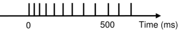
Neural spiking activity is a non-Gaussian system for which the concept of SNR has not been clearly defined. First, neuronal responses are point processes [2]-[4] because neurons represent and transmit information through their sequences of action potentials or spikes (Fig. 1). Second, defining what is the signal and what is the noise in the spiking activity of a neuron is a challenge. This is because the nature of the putative signal or stimulus for a given neuron differs appreciably between brain regions. For example, neurons in the visual cortex and the auditory cortex respond to features of light [5] and sound stimuli respectively [6]. In contrast, neurons in the rat hippocampus respond robustly to the animal’s position in its environment [7], while their counterparts in the monkey hippocampus respond to the process of task learning [8]. Third, in addition to responding to a putative stimulus, a neuron’s spiking activity is also modulated by biophysical factors such as its absolute and relative refractory periods, its bursting propensity, and local network and rhythm dynamics [9]. Hence, the definition of SNR must take account of the extent to which a neuron’s spiking responses are due to the signal or to these intrinsic biophysical factors.

500 Time (ms) 0

Fig. 1. The times of spikes (vertical bars) plotted on a time axis from a spike train.

the new estimator in simulation studies of a linear Gaussian system and neural spike trains.

II. THEORY

A. SNR for systems with a deterministic signal and additive Gaussian noise

Let Y be an n×1random vector and denote EY =η. We approximate η Xβ, where X is a matrix of non-random, known covariates and

n×p

β is an unknown p×1 parameter vector. We express Y in terms of Xβ with the linear relation Y =Xβ ε+ , where ε is a vector of independent, identically distributed Gaussian random errors with zero mean and variance

1

×

n

2

. ε

σ The signal-to-noise ratio for this model is

2 signal

σ

2 ,

SNR

ε

σ

( ) (T X ).

(1)

where the variance of the signal is

2 1

signal n X

σ = − β η− β η− (2)

A usual SNR estimate is computed as the ratio of the estimate of the variance of the signal to the variance of the noise. If we fit Y =Xβ ε+ , by least squares then the estimate of β is βˆ=(X XT )−1X yT and the estimated SNR is

ˆ) ( 1 ˆ

ˆ

( ) (

T

T

y X y X

y X y X

( 1 )

ˆ _,

ˆ)

SNR β β

β β

− −

− −

= (3)

where y1= y(1, ... ,1)T and 1

1

.

J

j j

y n− y

=

=

∑

Although we are unaware of studies of the statistical properties of this SNR estimator, work on a related statistic, the pseudo R-squared, has been reported and is discussed in IIE [17].

B. The SNR estimator in terms of the residual sums of squares

Under the linear model we define to be the expected squared prediction error when using the vector

( , ) (( ) (T ) | ) EPE Y η =E Y−η Y−η X

η to predict

the random vector Y and

2

( , ) (( ) (T ) | )

EPE Y Xβ =E Y−Xβ Y−Xβ X =nσ_ε is the expected squared prediction error when using Xβ to predict

Y

2

signal ( ( ) ) ( ( ) )

( ) ( ( ) ( )

( , ) ( , ).

T

T T

n E Y X E Y X

E Y Y Y X Y X

EPE Y EPE Y X

σ β β

[18]. It follows that

) E

η η β β

η β

= − −

= − − − −

= −

.

− (4)

We interpret (4) as the improvement in the prediction error obtained by using the covariateX We rewrite the true SNR in (1) as

2 signal

2

( , ) ( , ) . ( , ) EPE Y EPE Y X SNR

EPE Y X

ε

σ _{η β}

β σ

−

= =

( , ) EPE Y X

(5)

β can be estimated by

The term

ˆ ˆ

(y−Xβ) (T y−Xβ) and EPE Y( , )η can be estimated by (y−y) (T y−y), where βˆ=(XTX X y) T

.

is the minimum mean square (least-squares) estimate of β For the two prediction squared-error estimates the following relation holds

ˆ ˆ

( 1 ) ( 1 )

ˆ ˆ

( ) ( ) ( ) ( ),

T

T T

y X y X

y y y y y X y X

β β

β β

− −

= − − − − −

ˆ Model( , , )

ˆ Total( ) Residual( , , ),

SS y X

SS y SS y X

β

(6) or

β

= −

Total( )

SS y

ˆ Model( , , )

SS y X

(7)

where is the total variability in the data,

β is the variability in data explained by the signal estimateXβˆ and SSResidual( ,y X, )βˆ is the residual sum of squares which summarizes the variability in the data that is not explained by the signal estimate [19]. We rewrite the SNR estimate in (3) as

ˆ ˆ

( ) ( ) ( ) ( )

ˆ _,

ˆ ˆ

( ) ( )

T T

T

y y y y y X y X

SNR

y X y X

β β

β β

− − − − −

=

− −

(8)

or equivalently as

0

ˆ Model , , ˆ

ˆ Residual , ,

ˆ ˆ

Residual ,1, Residual , , , ˆ

Residual , ,

SS (y X )

SNR

SS (y X )

SS (y ) - SS (y X )

SS (y X )

β β

β β

β

=

=

(9)

0

ˆ where β =y.

C. Generalization of SNR to simultaneous signal and non-signal modulation of the mean

As above, we assume that Y =Xβ ε+ .

1 1 2 2,

X X X

However, now we assume that we can write β = β + β where X_{1 1}β is the component of the mean unrelated to the signal and

2 2

X β is the signal component of the mean. We have the partitions X =[X₁,X₂], β =(β β₁, ₂) ,T where X₁ is a

1

n×p matrix of non-signal covariates, X₂ is n×p₂ matrix of signal covariates, β₁ is vector of non-signal parameters and

1 1

p ×

2 p2 1

β is × vector of signal parameters. We have p1+p2= p.

* 1

β be the vector that gives the minimum Let

1 1).

X ( ,

EPE Y β It is defined as X_{1 1}β∗=E Y X[ | ₁].

*

( , 1 1) ( , ), ( , )

EPE Y X EPE Y X

SNR

EPE Y X

β β

β

∗ ₋

= (10)

where the numerator can be interpreted as the improvement in the expected prediction error of the signal, X_{2 2}β ,when controlling for the component of the mean X *

1β1 which is

unrelated to the signal. The denominator is the expected prediction error due to the noise. By analogy with (9) we can estimate the SNR in (10) as

1 ˆ1

Residual( , , ) Residual( , , )

ˆ _,

ˆ Residual( , , )

SS y X SS y X

SNR

SS y X

ˆ

β β

β

−

= (11)

where the numerator can now be interpreted as the variability in Y explained by the signal estimate X_{2 2}βˆ while controlling for the estimated effect of X_{1 1}βˆ and the denominator is the variability in Y due to noise. The estimates βˆ and βˆ₁ are obtained by computing separately the respective least-squares estimates of β and β₁ [19].

D. The SNR for generalized linear model systems We extend the SNR definitions presented in the previous sections to Generalized Linear Model (GLM) systems. GLM is an established statistical framework for performing regression analyses when the measured or observed data are not necessarily Gaussian [20]. GLM makes it possible to perform regression analyses to relate observations from any model in the exponential family to a set of covariates. This family includes well-known probability models such as the Gaussian, Bernoulli, binomial, Poisson, gamma and inverse Gaussian. GLM also provides an efficient way to compute the maximum likelihood (ML) estimates of the parameters for these models using iteratively re-weighted least squares. GLM methods are available in nearly every statistical package, and have the optimality properties and statistical inference framework common to all likelihood-based techniques [20]. We discuss here GLM systems in which the covariates may be partitioned into signal and non-signal components. All of the findings and statements below are valid for the linear Gaussian models in IIA-C, because they are GLMs.

We assume that f_β is a GLM probability model for a vector of observations Y and that in addition to we record observations from covariates that are summarized in the matrix

, Y

n p

.

n×p X We further assume that given a link functiong()we can express the expected value of Y given X as g E Y( ( |X)=Xβ =X1 1β +X2β2 where

1

X , β₁, X₂ and β₂ are defined in IIC. Let

1

fβ be a GLM with the covariate matrix X₁ and the parameter vector β₁. We also assume that g E( (Y X| ₁))=X_{1 1}β*, where β₁* is the vector that gives the minimum KL distance from the data to the model fβ. The vector β₁* can also be viewed as the probability limit of its ML estimator.

The generalization of the residual sum of squares for the linear model to GLM is the deviance defined as [20]

ˆ ( | ) ˆ

( , , ) 2 log ,

( | )

f y

Dev y X

f y y β β

β = −

ˆ

(12)

f

β is the ML estimate of β and

where ( | )y y

y

is the saturated model. The saturated model is the largest possible maximized likelihood. It is obtained by evaluating the parameters at the data [20]. The deviance is a measure of the distance between the model fβ and the observed data

or the saturated model. It can be viewed as giving an estimate of the “noise or residual sum of squares” for the GLM. The difference of deviances

y

1 ˆ1 ˆ

( , , ) ( , , ), Dev y X −Dev y X β

2 2ˆ

X (13)

β

gives the reduction in the deviance due to the signal β when controlling for the effect of the non-signal component

1 1ˆ ,

X β where βˆ₁ and βˆ are the ML estimates obtained from the two separate fits of the models *

1

f_β and f_β respectively to Equation 13 generalizes the numerator in (11). The difference of deviances in (13) is a likelihood ratio test statistic and an estimate of the improvement in Kullback-Leibler (KL) expected prediction error by the signal,

. y

2 2ˆ

X β when controlling for the effect of X_{1 1}βˆ [18]. This likelihood ratio is an estimator of

* 1 *

1

( )

( , ) ( , ) 2 log ,

( ) f Y EPE Y f EPE Y f E

f Y β β

β

β

⎡ ⎤

− = ⎢ ⎥

⎢ ⎥

⎣ ⎦

(14) [18]. We propose the following SNR measure as a generalization of (5 and 10)

( , 1) ( , )

( , ) EPE Y f EPE Y f SNR

EPE Y f

β . β

β

∗ −

=

SNR

(15)

We estimate the by the generalization of (11)

1 1

ˆ ˆ

( , , ) ( , , )

ˆ _.

ˆ ( , , ) Dev y X Dev y X SNR

Dev y X

β β

β −

= (16)

E. The bias of the SNR estimators

obtained data set, to evaluate the log-likelihood. Unfortunately, in many applications this approach is not feasible.

The numerator in (16) is a likelihood-ratio statistic

1 1

ˆ

2[log ( ,L y X, ) log ( ,β − L y X ,βˆ )] for testing the null hypothesis that the parameter vector β₂ is zero. In a GLM the likelihood-ratio statistic follows approximately a χ2 distribution with degrees of freedom under this null hypothesis

2 1

p = −p p

[20]. The approximate expectation of the likelihood-ratio statistic under H0 is therefore The

numerator of (16) is the same as the numerator in the pseudo R-squared measure for Poisson regression models. Like the R-squared in linear regression analysis, the pseudo R-squared approximates the fraction of the structure in the data explained by the Poisson regression model

2.

p

[17]. This idea led Mittlböck and Waldhör [17] to propose a bias correction of for the numerator of the pseudo R-squared for Poisson regression models. They validated use of this correction with simulation studies. By the same argument, the denominators in the SNR estimators have negative biases. It also suggests that the Mittlböck and Waldhör bias correction for the pseudo R-squared should provide a bias correction for the GLM SNR estimator (16) as well as for the other SNR estimators in (3), (8), and (11).

2 1

p = −p p

Therefore, if only one data set is available, we propose using the Mittlböck and Waldhör bias correction in the numerator and denominator of (16). That is, in (16) we correct the difference in the deviance in the numerator and the deviance in the denominator by the number of the parameters in the corresponding models to obtain the bias-corrected SNR estimator

1 ˆ1 ˆ 1

( , , ) ( , , )

ˆ _.

ˆ ( , , )

Dev y X Dev y X p p SNR

Dev y X p

β β

β

− +

=

+

−

(17)

Equation 17 is still a biased estimator because a ratio of unbiased estimators is not necessarily and unbiased estimator of a ratio. However, our simulations studies in the next section suggest that its bias is very small.

III. APPLICATIONS

We illustrate our proposed SNR estimator in an analysis of simulated data from a linear Gaussian model and simulated data from GLMs of spiking neurons.

A. SNR estimation for a linear Gaussian model

To illustrate the performance of our SNR estimator and its bias correction we study first the linear model Y =Xβ ε+ , where X is an n×2 matrix whose first column is a vector of ones, whose second column is the n×1 vector

and ( ₁, ₂)

T

(1 2 1 2 ...)

β = β β with β =₁ 1. The ε are independent, Gaussian random variables with zero mean and unit variance. We consider three values for the signal parameter β₂: 0, 0.3 and 1 which correspond to true SNR values of 0, 0.0225 and 0.250 respectively. The full model is Y Xβ ε, where

2 p

= +

= and the reduced model is Y=β₁+ε with p₁=1. For 400,

n= we simulated 10,000 samples from each model and compared the true SNR (1) with the traditional uncorrected SNR estimator (3) and our bias-corrected estimator (17).

For the models with β =₂ 0, 0.3 and1, the true values of the numerators in the SNR (1) are 0, 9 and 100, respectively. These values are overestimated by the numerator in (3) as 0.994, 1.05 and 1.2 re which are all close to our bias correction of p p₁ 1.

spectively

− = The true value of the denominator is 400 for all three models and it is underestimated by the denominator in (3) by approximately 2.025, 1.99 and 2.2 ectively. These are also close to our bias correction of p 2.

, resp

= In this example, the true values of the SNRs are consequently overestimated by the uncorrected estimators (3) or equivalently (16) by 0.003, 0.0019 and 0.006 respectively. In contrast, the biases in our corrected SNR estimators (17) are 0.00001, 0.0002 and 0.002

spectively.

Tru

2

re

e

β

True SNR

of the of the f the

SNR

f the

SNR Mean

uncorrected SNR estimates (3)

Mean corrected SNR estimates (17)

Bias o uncorrected

estimator

Bias o corrected

estimator

0 0.000 0.003 0.00001 0.003 0.00001

0.3 0.0225 0.0244 0.0227 0.0019 0.0002

1 0.250 0.256 0.252 0.006 0.002

Table 1. True values of the SNR (1) and SNR estimates for the three aussian models. The bias was evaluated in 10,000 simulated sam

G m

ples as the ean difference between the true value and the estimates.

ates Fig. 2 The histograms of uncorrected and corrected SNR estimates computed using 10,000 simulated samples from the three linear models with additive Gaussian noise and SNR=0 (first row), 0.0225 (second row) and 0.250 (third row). The uncorrected SNR estimates (first column) were calculated from (3) or equivalently (16). The corrected SNR estimates (second column) were calculated from (17). The bias corrected estimates improve the uncorrected estimates. In panel A the true SNR is zero yet, all of the uncorrected estim are strictly positive. The bold vertical line is the true SNR value.

0 0.05 0.1 0

200 400 600 800

0 0.02 0.04 0

1000 2000 3000 4000 5000

-0.010 0 0.01 0.02 0.03 0.04 1000

2000 3000 4000 5000

-0.050 0 0.05 0.1 200

400 600 800

0 0.2 0.4 0.6 0

200 400 600 800

0 0.2 0.4 0.6 0

200 400 600 800

A B

D C

E F

True SNR SNR Estimate SNR Estimate

Number of Es

timates

Uncorrected Bias-Corrected

Figure 2 illustrate the effect of the bias correction by showing the histograms of the SNR estimates obtained from the 10,000 simulated samples for the three signal plus noise models. The bias correction is most important for the data with a zero SNR (Fig. 2A, B). For the other two models with larger SNRs, the bias corrections do not change appreciably pared

fa estimated by m

the histograms of the SNR estimates (Fig. 2C, E com with 2D, F).

B. SNR estimation for GLMs of spiking neurons

To illustrate our method for a GLM system we consider two simulated neural spike trains modeled as point processes [1], [15], [3], [23], [24]. A point process is a time-series of 0-1 random events that occur in continuous time. For a neural spike train, the 1s are individual spike times and the 0s are the times at which no spikes occur. GLMs have been successfully used to formulate point process models that relate spiking activity to putative stimuli and biophysical ctors with the model parameters aximum likelihood [1], [3], [16], [24].

Given an observation interval (0, ],S let N t( ) be the number of spikes counted in interval (0, ]t for t∈(0, ].S A point proces

characterize

s model of a neural

d by its conditional function, spike train can be com intensity

pletely ( |t H_t),

λ

defined as

0

( |t H_t) lim P N t N t H

λ

Δ→

+ Δ − = =

Δ

( ( ) ( ) 1 | _t) (18) where H_t denotes the history of spikes up to time t [3] [4][23]. It follows from (18) that the probability of a single spike in a small interval ( ,t t+ Δ] is approximately

( |t H_t) .

λ Δ The conditional intensity function generalizes th

execution

e definition of the rate function of a Poisson process to a rate function that is history dependent.

Assume that a multiple-trial neurophysiology experiment is conducted with application of the same stimulus or

of the same task and neural activity is simultaneously recorded for K trials. We index the trials

1,..., .

k= K To obtain the di crete representation of the l intensity fun ion, we choose a large integer L and divide the trial interval S into subintervals of width

1

−

We choose large so that each subinterval contains at m spike. We index he subintervals

1,..,L

=

A an _k,A to be 1 if there is a spike in subi Δ] on trial k and is 0 otherwi We

..,n_{k L}} be the set of spikes on trial k, and s

conditiona . SL

Δ =

nterval let n_k ={n_k,1

1

{ ,...,

ct

ost on t

L n e d define ((A− Δ1) ,A

,

,. }

se.

K n= n

=

n be all of the spikes in the experiment. We let

1

, { , ,..., , 1}

k k p k

H _A n _A− n _A− denote the history of the spikes in trial k, up to time AΔ and p₁Δ is the amount of time in the past for which the history is relevant.

To analyze the neural spiking activity with define the con

a GLM ditional intensity function at trial at time

we

k AΔ

as [16], [24]

1 2

1 2 ,

1 , 2,

1 0

log ( | , , )

, ( ),

k k

p p

j k j r r

j r

H

n g

λ β β

β ₋ β

= =

Δ

=

∑

+

∑

Δ

A

A A

A

1 1 ( 1,1,..., 1,p)T

β = β β p₁×1

2 2 ( 2,0,..., 2,p )T

β = β β (p₂ 1) 1 (19)

where the first term describes the modulation of the spiking activity by the neuron’s biophysical properties i.e., the dependence of current spiking on recent spiking history, and the second term describes modulation of the neuron’s spiking activity by the signal or task. We have that

is a vector of biophysical

parameters and is an + ×

, , 1 2 ,

[ _k | _k , ] _k( | , , _k ) ,

E n H H

vector of signal parameters. In this GLM we have _{A A} β = λ AΔ β β _A Δ

() log().

and the link function is g = Under the discrete approximation to the point process likelihood the log-likelihood for this model is [1], [4], [16]

, , ,

1 1

log ( | )

log[ ( | , ) ] ( | , ) ,

K L

k k k k k

k

f n

n H H

β

λ β λ β

= =

=

∑∑

_A Δ _A Δ − Δ _A Δ

A

A A

1 2

( , ).

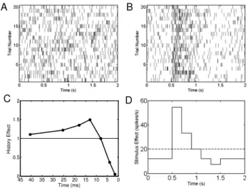
(20) where β = β β We simulated 20 two-second trials of spiking activity from two neurons (Figs. 3A, 3B).

Fig. 3. Two simulated spiking neurons. The spiking activity of the neuron in A has spike history dependence (C) and no task-specific (stimulus or signal) modulation (dashed horizontal line in D). The true SNR for this neuron is zero. The spiking activity of the neuron in B is modulated by spike history (C) and by the stimulus (solid curve in D). This neuron has an increased spike rate from 0.5-1 sec. The true SNR for this neuron is 0.0289.

The spiking activity of each neuron is modulated by the spike history effects (biophysical factors) described by the function in Fig. 3C. We modeled it by assuming a spike history dependence going back 50 msec based on [24] and represented it by choosing and by picking the components of

1 7

p =

1

β to capture the temporal dependence shown in Fig 3C. The coefficient β_1,1 represents the absolute refractory period (1-2 msec), coefficient β_1,2 models the relative refractory period (3-5 msec), coefficient β_1,3

0 5 10 15 20 25 30 35 2

40 45 0 0.5 1 1.5

Time (ms)

Hi

st

o

ry E

ff

e

c

t

A

D B

represents a period of no effect (6-10 msec) and coefficients

1,4 1,7

β −β (11-50 msec) represent increased spiking propensity. The spiking activity of the first simulated neuron is not modulated by the task (Fig. 3A, 3D horizontal dashed line), That is, β_2,0 =log 20 and β_2,r =0 for r=1,...,p₂. For this neuron the true value of the SNR is zero.

The spiking activity of the second simulated neuron (Fig. 3B) has both task-related dynamics (signal modulation) and spike history effects. The signal modulation is shown by an increase in spiking activity between at 0.5 to 1sec (Fig. 3D solid curve). We modeled this signal modulation by taking the g sr (19) to be orthogonal unit impulse functions each 100 msec in length and then defining the task-specific effect as a linear combination of these functions with the weights given by the

2 20

p =

2,r

β for (Fig. 3D, solid curve). The true value of the SNR for this neuron is 0.0289. We simulated each of the two neural spiking model 100 times. For each sample we calculated the uncorrected (16) and the corrected (17) SNR estimates. The biases of the uncorrected SNR estimates were 0.0022 and 0.0029 (Table 2), whereas the biases of the corrected SNR estimates were 0.0001 and 0.0003. Each of the means of the corrected SNR estimates is closer to the true SNR value.

1,..., 20.

=

r

Table 2. True values of the SNR and SNR estimates for two models of spiking neurons. Bias was computed from 100 simulations as the mean difference between the true value and the estimates.

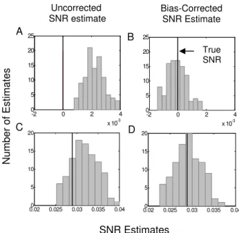
Figure 4 shows the distributions of the corrected and uncorrected SNR estimates. The uncorrected SNR estimates systematically overestimate the true SNR (Fig. 4, column one). For the first neuron (Fig. 4, row one) the true value of the SNR is zero. The histogram of the uncorrected SNR estimates is completely to the right of the true SNR value (Fig. 4A). For the second neuron (Fig. 4, row two) the true SNR is 0.0289. Approximately 75% of the uncorrected estimates are larger than the true value (Fig. 4C). For both neurons the corrected SNR estimates are centered almost exactly at their respective true SNR values (Figs. 4B, 4D). In summary, the uncorrected SNR estimator can have a large positive bias. This error is most critical for low SNR data.

IV. CONCLUSION

We have generalized the traditional estimator of the SNR to one appropriate for GLM systems. The new estimator uses the GLM concept of deviance to generalize the concepts of estimated signal variance and estimated noise variance for non-Gaussian systems. It also takes account of the effect on the SNR of non-signal covariates and the need for a bias correction. We applied the new estimator to simulated data from linear Gaussian models and to simulated data from point process models of neuronal spiking activity.

Neurons have very strong biophysical properties such as the absolute and relative refractory periods and bursting propensity. These properties affect how the neuron represents and transmits information about a stimulus (signal). In most current analyses of neural responses to a signal these properties are not considered. Nevertheless, these biophysical properties contribute in a structured, non-random way to the fluctuations in the neural response. Hence, they should not be considered as noise but must be taken into account (corrected for) to assess properly the effect of the signal on the neural response. By incorporating the bias correction our SNR estimator (17) does not increase with the addition of unimportant covariates. Our bias-corrected SNR estimator can give negative values when the true SNR is at or close to zero, suggesting a very low SNR system. The SNR for the simulated neuron of 0.0289 (-15.4 dB) is typical of preliminary results we have obtained from the analysis of actual spiking neurons [25].

Fig. 4 Histograms of the SNR estimates in 100 simulations of the zero SNR (first row) and 0.0289 SNR model (second row) of neural spiking neuron. The bold vertical line is the true SNR value.

Our new SNR estimator is applicable to any system in which the data can be modeled using GLM. We are currently working on constructing confidence intervals for the estimator and on applying it in analyses of actual neural systems. Our SNR estimator may also have important implications outside of neuroscience because it can be extended to analyze any system in which response modulation by distinct signal components can be expressed as separate components of a likelihood function.

ACKNOWLEDGMENT

G.C. thanks Professor Leslie Smith from University of Stirling and Dr. Yunfei Chen from University of Warwick for helpful discussions. We thank Julie Scott for invaluable technical assistance with the manuscript preparation.

Effect of stimulus or signal

True SNR (15)

Mean of uncorrected SNR estimate (16)

Mean of corrected SNR estimate (17)

Bias of uncorrected SNR estimate

Bias of corrected SNR estimate

Absent 0 0.0022 0.0001 0.0022 0.0001

Present 0.0289 0.0318 0.0292 0.0029 0.0003

-2 0 2 4

x 10-3 0

5 10 15 20 25

0.020 0.025 0.03 0.035 0.04 5

10 15 20

-2 0 2 4

x 10-3 0

5 10 15 20 25

A

D C

B

True SNR

Uncorrected SNR estimate

Bias-Corrected SNR Estimate

Number of Es

timates

SNR Estimates

0.02 0.025 0.03 0.035 20

15

10

5

REFERENCES

[1] Chen Y, Beaulieu NC. Maximum likelihood estimation of SNR using digitally modulated signals. IEEE Trans. Wireless Comm, 6(1), 2007. [2] Brillinger DR. Maximum likelihood analysis of spike trains of

interacting nerve cells. Biol. Cybern. 59: 189-200, 1988.

[3] Brown EN, Barbieri R, Eden UT, and Frank LM. Likelihood methods for neural data analysis. In: Feng J, ed. Computational Neuroscience: A

Comprehensive Approach. London: CRC, Chapter 9: 253-286, 2003.

[4] Brown EN. Theory of Point Processes for Neural Systems. In: Chow CC, Gutkin B, Hansel D, Meunier C, Dalibard J, eds. Methods and

Models in Neurophysics. Paris, Elsevier, Chapter 14: 691-726, 2005.

[5] MacEvoy SP, Hanks TD, Paradiso MA Macaque V1 activity during natural vision: effects of natural scenes and saccades, J. Neurophys. 99: 460-472, 2008.

[6] Lim HH, Anderson DJ. Auditory cortical responses to electrical stimulation of the inferior colliculus: implications for an auditory midbrain implant. J. Neurophys. 96(3):975-88, 2006.

[7] MA Wilson MA, McNaughton BL Dynamics of the hippocampal ensemble code for space. Science, 26:1055-1058,1993.

[8] Wirth S, Yanike M, Frank LM, Smith AC, Brown EN, Suzuki WA. Single neurons in the monkey hippocampus and learning of new associations. Science 300: 1578-1584, 2003.

[9] Dayan P, and Abbott L. Theoretical Neuroscience, Oxford University Press, Oxford, 2001.

[10] Shadlen, MN and Newsome, WT. The variable discharge of cortical neurons: implications for connectivity, computation, and information coding. J. Neurosci. 18(10): 3870-3896, 1998.

[11] Softky WR, Koch C. The highly irregular firing of cortical cells is inconsistent with temporal integration of random EPSP’s. J. Neurosci.

13:334-350, 1993.

[12] Teich MC, Johnson DH, Kumar AR, Turcott RG. Rate fluctuations and fractional power-law noise recorded from cells in the lower auditory pathway of the cat. Hear Res. 46:41–52, 1990.

[13] Optican LM, Richmond BJ. Temporal encoding of two-dimensional patterns by single units in primate inferior temporal cortex. III. Information theoretic analysis. J. of Neurophysiol., 57(1), 162-178, 1987.

[14] Rieke F, Warland D, de Ruyter van Steveninck RR, Bialek W. Spikes:

exploring the neural code. MIT Press, Cambridge, USA, 1997.

[15] Kass RE and Ventura V. A spike train probability model. Neural

Comput. 13: 1713-1720, 2001.

[16] Truccolo W, Eden UT, Fellow MR, Donoghue JP, Brown EN. A point process framework for relating neural spiking activity to spiking history, neural ensemble and extrinsic covariate effects. J. Neurophys. 93: 1074-1089, 2005.

[17] Mittlböck M, Waldhör T. Adjustments for R2-measures for Poisson regression models. Computational Statistics and Data Analysis 34: 461-472, 2000.

[18] Hastie T. A Closer Look at the Deviance, The American Statistician, Vol 41, No 1, pp 16-20, 1987.

[19] Neter J, Kutner MH, Nachtsheim CJ, Wasserman W. Applied Linear

Statistical Models. 4th ed, McGraw-Hill, 1999.

[20] McCullagh P, Nelder A. Generalized Linear Models, 2nd ed., Chapman & Hall, 1989.

[21] Kitagawa G, Gersch W. Smoothness Prior Analysis of Time Series.

New York: Springer-Verlag, 1996.

[22] Pawitan Y. In All Likelihood. Oxford University Press. 2001. [23] Daley D and Vere-Jones D. An Introduction to the Theory of Point

Process. 2nd ed., Springer-Verlag, New York, 2003.

[24] Czanner G, Eden UT, Wirth S, Yanike M, Suzuki WA, Brown EN. Analysis of between-trial and within-trial neural spiking dynamics. J.

Neurophys., (Epub, Jan. 23) 2008, In Press.