Estimate of the atmospheric turbidity from three broad-band solar radiation algorithms. A comparative study

SRef-ID: 1432-0576/ag/2004-22-2657 © European Geosciences Union 2004

Annales

Geophysicae

Estimate of the atmospheric turbidity from three broad-band solar

radiation algorithms. A comparative study

G. L´opez and F. J. Batlles

Departamento de Ingenier´ıa El´ectrica y T´ermica, EPS La R´abida, Universidad de Huelva, Ctra. Palos de la Frontera s/n., 21819 Huelva, Spain

Received: 5 December 2003 – Revised: 26 February 2004 – Accepted: 30 March 2004 – Published: 7 September 2004

Abstract. Atmospheric turbidity is an important parameter for assessing the air pollution in local areas, as well as being the main parameter controlling the attenuation of solar radi-ation reaching the Earth’s surface under cloudless sky con-ditions. Among the different turbidity indices, the ˚Angstr¨om turbidity coefficientβ is frequently used. In this work, we analyse the performance of three methods based on broad-band solar irradiance measurements in the estimation ofβ. The evaluation of the performance of the models was under-taken by graphical and statistical (root mean square errors and mean bias errors) means. The data sets used in this study comprise measurements of broad-band solar irradiance ob-tained at eight radiometric stations and aerosol optical thick-ness measurements obtained at one co-located radiometric station. Since all three methods require estimates of precip-itable water content, three common methods for calculating atmospheric precipitable water content from surface air tem-perature and relative humidity are evaluated. Results show that these methods exhibit significant differences for low val-ues of precipitable water. The effect of these differences in precipitable water estimates on turbidity algorithms is dis-cussed. Differences in hourly turbidity estimates are later examined. The effects of random errors in pyranometer mea-surements and cloud interferences on the performance of the models are also presented. Examination of the annual cycle of monthly mean values ofβ for each location has shown that all three turbidity algorithms are suitable for analysing long-term trends and seasonal patterns.

Key words. Atmospheric composition (aerosols and parti-cles; transmission and scattering of radiation) – Meteorology and atmospheric dynamics (radiative processes)

1 Introduction

Atmospheric turbidity is associated with atmospheric aerosol load. Aerosols are solid and liquid particles suspended in the atmosphere, ranging in size from 10−3_{µm to several tens}

Correspondence to:G. L´opez ([email protected])

of microns. These particles are either of natural sources (such as volcanic eruptions, dust storms, forest and grass-land fires, sea spray, etc.) or of anthropogenic origin (such as the burning of fossil fuels). An increase in the concen-tration of aerosols in some urban regions caused by human activity has a significant impact on the environmental quality of the cities, which makes the air turbid with lower visibil-ity, the atmospheric opto-chemistry faster, and the air pol-luted. In addition, aerosols play an important role in absorp-tion and scattering of solar radiaabsorp-tion, as well as in the physics of clouds and precipitation. Therefore, atmospheric turbidity is not only an important factor for monitoring the air pollu-tion, but also in meteorology, climatology and for designing of solar energy systems.

Due to the relationship existing between aerosols and at-tenuation of solar radiation reaching the Earth’s surface, dif-ferent turbidity factors based on radiometric methods have been defined to evaluate the atmospheric turbidity. Some of these are the Linke turbidity factor, TL (Linke, 1922), the

˚

Angstr¨om turbidity parameters,αandβ ( ˚Angstr¨om, 1929), the Sh¨uepp coefficient, B (Sh¨uepp, 1949), the Unsworth-Monteith turbidity factor,TU(Unsworth and Monteith, 1972) and the horizontal visibility. Among them, ˚Angstr¨om turbid-ity parameters are commonly used. They were defined by

˚

Angstr¨om (1929) through the relation

τa(λ)=βλ−α, (1)

et al., 1998). However, these spectral measurements have only recently been established and the sparseness of this data both spatially and temporally makes it impossible to study current long-term turbidity trends. To circumvent this limi-tation, several methods based on broad-band measurements of solar radiation and related atmospheric parameters can be used in the first place (Louche et al., 1987; Pinazo et al., 1995; Gueymard and Vignola, 1998; Power, 2001). These methods estimate the turbidity coefficient β and assume a constant value for the wavelength exponentα, which is of-ten set to 1.3, following the reference value originally pro-posed by ˚Angstr¨om for continental aerosols. This assump-tion is needed due to the unavailability of measurements of the wavelength exponent.

In this work, three methods for estimating the turbidity coefficientβ from broad-band solar radiation data are com-pared. They were formulated by Dogniaux (1974), Louche et al. (1987) and Gueymard and Vignola (1998), respectively. The first two were selected because of their simplicity and extensive use in order to either estimate solar radiation com-ponents from parametric models or to study seasonal turbid-ity variations (Sinha et al., 1998; Pedr´os et al., 1999; Batlles et al., 2000; Li and Lam, 2002; Janjai et al., 2003), whereas the third one is new. It is important to note that these tur-bidity algorithms need knowledge of total precipitable water in the atmosphere, in order to take into account the deple-tion of incident solar radiadeple-tion due to this component. This information may be obtained from radiosonde soundings or from measurements of spectral solar radiation in water va-por absorption bands. However, these measurements are of-ten unavailable at a specific site. For this reason, alternative methods have been proposed to estimate precipitable water content from surface conditions using correlations with pa-rameters such as dew point temperature or using equations based on temperature and relative humidity (Iqbal, 1983). These correlations are possible because atmospheric water vapor is strongly concentrated in the lower atmospheric lay-ers (Viswanadham, 1981). Among the existing formulas, Leckner’s approach (Leckner, 1978) and the Reitan based formula reported by Wright et al. (1989) are widely em-ployed. More recently, Gueymard (1994) has reported a new approach to calculate precipitable water based on the rela-tionship between the water vapor scale height and tempera-ture. In general, each of these approaches provides different precipitable water values, which can lead to over/under esti-mation of turbidity levels. For this reason, in Sect. 4 a study is initially carried out to analyse the differences on precip-itable water calculated by means of several methods and how the selected turbidity algorithms are affected by these differ-ences. In Sect. 5, turbidity estimates by each selected algo-rithm are first compared with each other. Next, broad-band turbidity estimates are compared with experimental values derived from sunphotometric measurements. Lastly, the an-nual cycle of monthly mean values of the coefficientβ cal-culated by each turbidity algorithm is examined in climato-logically diverse regions.

2 Experimental Data

2.1 Broadband solar irradiance measurements

In order to estimate the turbidity coefficient by means of broad-band algorithms, data collected at eight radiometric stations were used. Table 1 summarises their geographical locations, the number of hours and the recording period. The stations were chosen with the intention of best representing a wide diversity of climates. In this sense, Almer´ıa’s sta-tion is located on a seashore site on the Mediterranean coast of southeastern Spain. High frequency of cloudless days, an average annual temperature of 17◦_{C, and the persistence} of high humidity characterise the local climate. Granada’s station is located on the outskirts of Granada (southeastern Spain). Cool winters and hot summers characterise this in-land location. The U.S. stations are part of NOAA’s Surface Radiation budget network – SURFRAD – (Augustine et al., 2000). They represent inland locations with different regimes of continental climate.

All data sets contain measurements of global and diffuse solar irradiance on a horizontal surface, temperature and rel-ative humidity. Measurements of surface albedo and atmo-spheric pressure at ground level are also available at the SURFRAD stations. Kipp and Zonen pyranometers (model CM-11) were employed to measure the global solar irra-diance at the Almer´ıa and Granada stations, whereas Epp-ley ventilated pyranometers model PSP were employed for both down- and upwelling global and diffuse irradiance at the SURFRAD stations. At Almer´ıa’s and Granada’s sta-tions, diffuse irradiance was measured by a Kipp and Zo-nen pyranometer (model CM-11) equipped with an Eppley shadow band model SBS. Because the shadow band screens the sensor from a portion of the incident diffuse radiation coming in from the sky, a correction was made to the mea-surements following Batlles et al. (1995). The SURFRAD stations used Eppley pyranometers mounted on Eppley auto-matic solar trackers model SMT-3 equipped with shade disks model SDK. Measurements of temperature, relative humid-ity and surface pressure were also made.

Data were recorded and averaged over different sampling intervals (1, 3, 5 and 10 min). Values of direct irradiance were obtained from a difference of measured global and dif-fuse irradiance. Next, hourly mean values were calculated for all variables. Due to cosine response problems of radio-metric sensors, we have only used cases corresponding to solar elevations higher than 5◦_{. Finally, data associated with} cloudless sky conditions were selected. To identify cloud-less conditions, we used the normalised clearness indexk′ t proposed by Perez et al. (1990):

k′_t = kt

1.031 exp_0.9+−1_9..₄4_/m

a,

+0.1

(2)

Table 1. Geographical locations of the radiometric stations, period of measurement and number of hours associated with cloudless sky conditions.

Station Abbrev. Country Latitude (◦N) Longitude (◦O) Altitude (a.m.s.l.) Years Hours

Almer´ıa ALM Spain 36.83 2.41 0 1990–1998 12 880

2052*

Bondville BON US (IL) 40.06 88.37 213 1996–1999

611**

Desert Rock DRA US (NV) 36.63 116.02 1007 1998–1999 3440

Fort Peck FPK US (MT) 48.31 105.10 634 1996–1999 2815

Goodwin Creek GWN US (MS) 34.25 89.87 98 1995–1999 2885

Granada GRA Spain 37.18 3.58 660 1994–1995 3730

Penn State PSU US (PA) 40.72 77.93 376 1998–1999 1190

Table Mountain TBL US (CO) 40.13 105.24 1689 1995–1999 5878

* – Broad-band solar irradiance data ** – AOT data

Kasten (1966) and corrected for local atmospheric pressure (Iqbal, 1983). A cloudless sky is then defined as k′_t>0.7 (Molineaux et al., 1995). Obviously, some data may be er-roneously included as a totally cloud-free atmosphere using this simple radiometric criterion. It is thus expected that this method does not detect, for instance, thin cloud covers as those due to cirrus clouds, which would have little effect on the measured global irradiance. Under these conditions, un-realistic higher turbidity levels would be observed.

2.2 Spectral aerosol optical thickness data

A second data set including aerosol optical thickness (AOT) at 0.440, 0.500, 0.640 and 0.870µm were extracted from the automated Cimel CE-318 belonging to the AERONET and located at the Bondville radiometric station. The record-ing period was selected to match the SURFRAD broad-band radiation measurements from August 1996 through August 1999. The selected data corresponds to the quality assured level (Level 2.0) provided by the AERONET. Since sev-eral measurements per hour are available, hourly averaged values were obtained. Next, Bondville’s AERONET and SURFRAD data sets were combined in such a way that their hourly values matched each other. A first filter was applied using Eq. (2) to select cloudless conditions, obtaining a data set with 1278 h. To assure a totally cloud-free data set, from these days we performed a visual inspection on the daily evo-lution of the broad-band direct, diffuse and global irradiances recorded every 3 min, screening out those suspected hours. After applying this second visual filter, a quality-controlled data set with 611 hourly averaged records was obtained.

Assuming α is constant throughout a given wavelength range, values ofαandβ were derived by linear fit from the four AOT values taking in Eq. (1) natural logarithm:

lnτ (λ)=lnβ−αlnλ. (3)

Values of α and β calculated from AOTs data and using Eq. (3) will be referred to asαsunphot andβsunphot, respec-tively.

3 Description of the algorithms to calculate coefficientβ

All three models considered herein (Dogniaux, 1974; Louche et al., 1987; Gueymard and Vignola, 1998) are well estab-lished. They have been adequately described in sufficient de-tail in the previously cited references. For the sake of clarity these models are described briefly in the following segment. Hereafter, we refer to each model by the name of the first author.

3.1 Dogniaux’s algorithm

Dogniaux (1974) derived the following empirical relation for estimating Linke’s turbidity factor using inputs of solar ele-vationh(in degrees), precipitable water contentw(in cm), and ˚Angstr¨om’s turbidity coefficientβ:

TL=

85+h

39.5e−w_+47.4 +0.1

+(16+0.22w)β. (4) The Linke turbidity factor is defined as the number of Rayleigh atmospheres (an atmosphere clear of aerosols and without water vapor) required to produce a determined atten-uation of direct radiation. This turbidity factor is related to measures of direct irradianceIn by means of the following equation:

TL= 1 δRma

ln _I

0 In

, (5)

where I0 is the extraterrestrial normal irradiance andδR is the Rayleigh optical thickness. By using Eqs. (4) and (5),

˚

0 1 2 3 4 5 -15

-12 -9 -6 -3 0 3 6 9 12

w

W1 - wG

w

W2 - wG

w

L - wG

∆

w

(%)

w_{G (cm)}

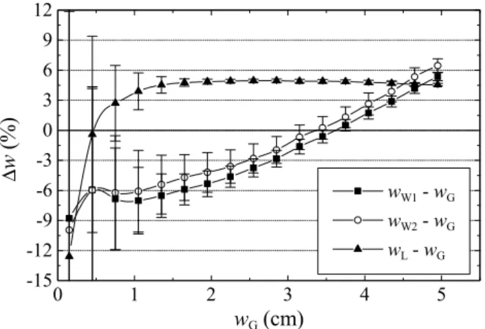
Fig. 1.Average relative differences of precipitable water estimated by Wright’s (using two different algorithms to calculate Td,wW1 andw_W2), Leckner’s(wL) and Gueymard’s(wG)methods against precipitable water estimated by Gueymard’s method.

was calculated using the formula proposed by Kasten (1980). Previous analyses have shown that the use of the new equa-tion given by Louche et al. (1986) and corrected by Kasten (1996) seems to be unsuitable to estimateβ from Eqs. (4) and (5). We refer to coefficientβcalculated by means of this method asβD.

3.2 Louche’s algorithm

The method proposed by Louche et al. (1987) was derived from the model C by Iqbal (1983), but using the expression by M¨achler (1983) for the transmittance due to aerosol at-tenuation. The ˚Angstr¨om turbidity coefficient obtained by Louche et al. (1987),βL, is expressed as:

βL= 1 maD

ln

_C

A−B

, (6)

where

A= In

0.9751I₀TrToTgTw

, (7)

B=0.12445α−0.0162, (8)

C=1.003−0.125α, (9)

D=1.089α+0.5123. (10)

The transmittances by Rayleigh scattering (Tr), ozone (To), uniformly mixed gases (Tg) and water vapor (Tw) are given by the parametric model C by Iqbal (1983). The transmit-tancesTr andTgdepend on air mass only; the transmittance Toneeds information on ozone content, which may be calcu-lated from location and time (Van Heuklon, 1979); the trans-mittance by water vaporTw uses air mass and precipitable water content as inputs. A value ofαequal to 1.3 is assumed.

3.3 Gueymard’s algorithm

From the spectral code SMARTS2 (Gueymard, 1995), Guey-mard and Vignola (1998) proposed a method for estimating coefficientβ using measurements of global (or diffuse) and direct irradiance. The equation obtained is as follows:

βG=

q

a₁2−4(a₂−a₃Kdb)(a0−Kdb) 2(a2−a3Kdb)

, (11)

where the coefficientsaidepend on air mass and precipitable water. Kdb is the standardised value (to zero altitude and total column ozone equal to 0.3434 atm-cm) of the ratio be-tween diffuse and direct irradiance. Equation (11) is valid for valuesβG≤0.4 and for a surface albedo equal to 0.15. A cor-rection is necessary if surface albedo is different (Gueymard and Vignola, 1998). The main novel feature of this method is an almost null dependence on precipitable water content. On the other hand, it is interesting to note that this param-eterisation ofβ is based on a fixed value ofαequal to 1.3. Thus, this algorithm would at first be useful only for those locations with those aerosol characteristics. This limitation will be analysed in Sect. 5.2.

4 Influence of differences in calculating precipitable water on turbidity estimates

Total precipitable waterw is defined as the vertically inte-grated water vapor in a column extending from the surface to the top of the atmosphere. In order to estimate the turbidity coefficientβfrom broad-band solar radiation measurements, knowledge of total precipitable water in the atmosphere is needed. In the absence of an atmospheric sounding or solar spectral measurements, the linear relationship between the logarithm ofwand dew point temperatureTd, has been often used to calculate precipitable water (Iqbal, 1983):

lnw=a+bTd. (12)

Parametersaandbare not universal and thus they should be calculated for every place and for a specific sampling time. Nevertheless, several authors (Molineaux et al., 1995; Mot-tus et al., 2001; Marion and George, 2001; Lopez et al., 2001) have employed Eq. (12) using those values of the parameters obtained for Albany NY by Wright et al. (1989),a=−0.0756 andb=0.0693, and which were suitable for estimating in-stantaneous precipitable water under cloudless skies. In ad-dition to the errors of estimate associated with local param-etersaandb, a second source of error is due to the method of calculating dew point temperature. In general terms,Tdis related to temperatureT and relative humidity8by means of saturation pressure of water vaporps:

1989) or calculated from some formulas proposed in the lit-erature. This second option is more suitable for computing calculations. Gueymard (1993) analysed a wide variety of such algorithms. Among those, the Magnus type and Leck-ner equations are common expressions used for calculating ps. They read, respectively, as:

p(sMagnus)=6.107 exp

17.38T 239+T

1_{, (14)}

p(_sLeckner)=0.01 exp

26.23− 5416

273.15+T

, (15)

where ps is expressed in mbar and T in degrees Celsius. Usingps(Magnus)or p(sLeckner) in Eq. (13), different relations between dew point temperature and surface temperature and relative humidity are thus obtained:

T_d(Magnus) = 239f (T , 8)

17.38−f (T , 8) ,

f (T , 8)=ln8+ 17.38T

239+T

, (16)

T_d(Leckner)= 5416

5416/(T +273.15)−ln(8) −273.15, (17) where relative humidity is in fractions of one. Precipitable water calculated by using Wright’s formula and dew point temperature estimated by Magnus’ or Leckner’s equation is referred to aswW1andwW2, respectively.

Another alternative method often used to calculate the amount of precipitable water is given by Leckner (1978). Leckner’s correlation expresses the precipitable water in terms of relative humidity:

wL=49.3

8ps(Leckner)

T , (18)

whereT is in Kelvin. More recently, Gueymard (1994) in-troduced a new relationship betweenwand the surface tem-perature and relative humidity given by:

wG=21.67Hv

8p(sGueymard)

T , (19)

whereps(Gueymard) 2 andHv are, respectively, given by the following formulas:

lnps(Gueymard)=22.33−49.14 1 T0

−10.922 1

T₀2 −0.3902T0

, (20)

Hv=0.4976+1.5265θ+exp(13.6897θ−14.9188θ3)(21) 1_{The new constants are given by Gueymard (1993).}

2_{The coefficients of lnp}(Gueymard)

s have been rounded off from their original values in order to simplify this expression. Relative errors of this modifiedps with regard to the originalps values by Gueymard (1994) are lower than 0.035% for temperature values ranging from−40 to 60◦C.

0 1 2 3 4 5

-10 -8 -6 -4 -2 0 2 4 6 8 10

a) Dogniaux

βD(wW1) - βD(wG)

βD(wW2) - βD(wG)

βD(wL) - βD(wG)

∆

β

(%

)

w

G (cm)

0 1 2 3 4 5

-10 -8 -6 -4 -2 0 2 4 6 8 10

b) Louche

βL(wW1) - βL(wG)

βL(wW2) - βL(wG)

βL(wL) - βL(wG)

∆

β

(%)

w

G (cm)

0 1 2 3 4 5

-10 -8 -6 -4 -2 0 2 4 6 8 10

c) Gueymard

βG(wW1) - βG(wG)

βG(wW2) - βG(wG)

βG(wL) - βG(wG)

∆

β

(%

)

w

G (cm)

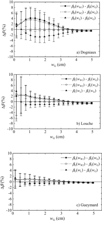
Fig. 2. Average relative differences (as legends inside of the fig-ures refer to) against precipitable water calculated by Gueymard’s method for each turbidity algorithm.

where T₀=T /100, θ=T /273.15 and T is expressed in Kelvin.

Leckner’s equation for calculating dew point temperature implies differences lower than 1.5% on the values of pre-cipitable water estimated by means of Wright’s correlation. In fact, average deviations betweenT_d(Magnus)andT_d(Leckner) are less than 0.2◦_{C. Since deviations on precipitable} wa-ter calculated by means of Wright’s correlation is given by 1wW=0.0693w 1Td, average differences around 0.2◦C on Td leads to relative errors lower than 1.5%. ForwG>1 cm, relative differences between Wright’s correlation and Guey-mard’s method present a linear trend ranging from−6% to 6%. The use ofT_d(Leckner) in Wright’s correlation provides estimates slightly closer to those from Leckner’s and Guey-mard’s approaches than those corresponding to the use of T_d(Magnus). On the other hand, relative differences between Leckner’s approach and Gueymard’s method present an al-most constant value around 4−5% for this region of pre-cipitable water. Since the spectral absorption bands of wa-ter vapor rapidly saturate as the amount of wawa-ter vapor in-creases, these differences are expected to be of minor rel-evance in estimatingβ. For 0.5<w_G<1 cm, Leckner’s ap-proach provides average values closer to those by Guey-mard’s method with respect to Wright’s correlation. How-ever, both Leckner’s and Wright’s approach exhibit large standard deviations, which may lead to an inverse situation under several local atmospheric conditions. ForwG<0.5 cm, Wright’s and Leckner’s algorithms present average relative differences around−9% and−13%, respectively, and higher standard deviations with respect to Gueymard’s method. Dif-ferences between Leckner’s and Gueymard’s methods to cal-culate precipitable water agree with those reported by Guey-mard and Garrison (1998) for Montreal.

In order to analyse the influence of precipitable wa-ter differences on turbidity estimates by using Dogniaux’s, Louche’s and Gueymard’s approaches independently, the fol-lowing relative differences between turbidity estimates1βi for every one of these approaches (i=D, L or G) and employ-ing, respectively each of the above precipitable water meth-ods were obtained:3.

1βi =

βi(wj)−βi(wG)

βi(wG)

, (22)

where j (=w_W1,w_W2orw_L)refers to the precipitable water method used.

Figure 2 shows the average relative differences (expressed as percentage) againstw_Gfor each turbidity approach. Stan-dard deviations of the mean are also included. It is noted that the three turbidity methods present a negligible dependence on precipitable water differences for higher precipitable wa-ter values, as was expected. AswGdecreases, Gueymard’s turbidity method provides the lowest values of the average turbidity relative differences and standard deviations with a slight increase in standard deviation. Average turbidity rel-ative differences and standard deviations from Louche’s al-gorithm present a trend similar to those from Gueymard’s

3_{Relative differences corresponding toβ(w}

G)<0.002 were

re-moved to avoid large values of1βi.

method but standard deviations are dramatically increased asw_G decreases below 0.7 cm. On the other hand, Dogni-aux’s method presents the higher increase in average turbid-ity relative differences and standard deviations asw_Granges from 2.5 cm to 0.7 cm; asw_Gdecreases below 0.7 cm, these values are not strongly affected for the large increase in precipitable water relative differences and standard devia-tions. Therefore, these results point to Gueymard’s turbidity method to be the less dependent on precipitable water differ-ences, whereas Dogniaux’s and Louche’s methods appear to be more sensitive to the precipitable water method selected for 0.7<wG<2.5 cm andwG<0.7 cm, respectively.

5 Comparison of the turbidity algorithm performances

5.1 Comparison procedure 1

The comparison of the performance of the turbidity algo-rithms was initially undertaken by analysing the correspond-ing turbidity estimates between each other. For that and here-after, all three methods used precipitable water estimates by Gueymard’s approach. Figure 3 shows turbidity values cal-culated, respectively, by Dogniaux’s and Gueymard’s algo-rithms against those estimated by Louche’s algorithm using the whole database. For a better comparison, the coefficient of determination r2, the root mean square error RMSE and the mean bias error MBE between y- and x-values are also included. These statistical tests were computed as an aver-age of each r2, RMSE and MBE value calculated separately at each location. In addition, the standard deviation of each statistical test is added as well. Standard deviation provides information about how tightly all the independent values are clustered around the mean and thus how representative the statistical tests are for every location.

From Fig 3a, it may be seen that the simple Dogniaux’s correlation provides hourly turbidity estimates quite similar to those calculated by Louche’s algorithm, with a higher co-efficient of determination r2=0.973±0.006. The low stan-dard deviation means this result is highly representative and thus, a good match between both turbidity estimates is ex-pected for every location. The mean value of the MBE equal to 0.003±0.007 denotes turbidity values by Dogniaux’s cor-relation overestimate slightly those obtained using Louche’s algorithm at most locations. However, the higher standard deviation with respect to the mean value points out the oppo-site tendency was found at some locations.

A more detailed analysis of the differences β_D−β_L has shown that these differences exhibit a similar dependence on precipitable water at each locations, such as it is derived from Fig. 4. After removing this dependence, it could be expected that turbidity estimates by Dogniaux’s correlation and those by Louche’s algorithm present closer hourly values to each other. For that, the following quadratic-fitted curve was ob-tained using all average differences from each location other than Table Mountain

0.0 0.1 0.2 0.3 0.4 0.5 0.6 0.7 0.0

0.1 0.2 0.3 0.4 0.5 0.6 0.7

(a)

r² = 0.973 ± 0.006 MBE = 0.003 ± 0.007 RMSE = 0.012 ± 0.003

β

β

0.0 0.1 0.2 0.3 0.4 0.5 0.6 0.7 0.0

0.1 0.2 0.3 0.4 0.5 0.6 0.7

(b)

r² = 0.92 ± 0.02 MBE = -0.004 ± 0.004 RMSE = 0.020 ± 0.002

β

β

Fig. 3. Comparison between hourly turbidity estimates by using Dogniaux’s, Louche’s and Gueymard’s algorithms.

0 1 2 3 4 5

-0.02 -0.01 0.00 0.01 0.02 0.03

fitted curve ALM BON DRA FPK GRA GWN PSU TBL

β

-

β

w

_(cm)

Fig. 4.Average differences between turbidity estimates by Dogni-uax’s correlation and Louche’s algorithm versus precipitable water by Gueymard’s approach for each location.

Figure 5 showsβ_D′ = βD−1βD−L versusβL. Statistical tests in the above sense are also included. It may be seen that the spread of the data points is reduced. Indeed, the new

co-0.0 0.1 0.2 0.3 0.4 0.5 0.6 0.7

0.0 0.1 0.2 0.3 0.4 0.5 0.6 0.7

r² = 0.994 ± 0.004 MBE = 0.001 ± 0.003 RMSE = 0.006 ± 0.002

β

'

β

Fig. 5. Comparison between hourly turbidity estimates by using Dogniaux’s correlation modified by Eq. (22) and Louche’s algo-rithm.

efficient of determination is increased from 0.973 to 0.994, and the corresponding standard deviation is slightly dimin-ished. The MBE and RMSE (along with the corresponding standard deviations) are also reduced with values equal to 0.001±0.003 and 0.006±0.002.

On the other hand, Louche’s and Gueymard’s algorithms present higher differences to each other as it is derived from Fig. 3b and the values of the statistical test. The relationship between both turbidity estimates presents a higher spread of the data points such as the lower coefficient of determination (r2=0.92±0.02) and the higher RMSE (0.020±0.002) prove. In addition to the different formulation of both algorithms, a second source leading to this spread is associated with cloud interference affecting in a different way the estimates ofβ, which is not present between Dogniaux’s and Louche’s meth-ods. This assumption will be analysed in the next section. A mean value of the MBE equal to−0.004±0.004 denotes Gueymard’s approach underestimatesβ values with respect to Louche’s algorithm for almost every locations. It is in-teresting, however, to note that Gueymard’s approach tends to overestimate the turbidity values calculated by Louche’s algorithm in the region of higher turbidity levels at each lo-cation. This result would be again associated with cloud in-terference. In this sense and such as it was noted earlier, the use of hourly global irradiance data alone to identify cloud-less skies is not sufficient to provide a totally cloud free at-mosphere which is needed for an accurate performance of Gueymard’s algorithm.

-10

-5

0

5

10

0

20

40

60

80

100

(a)

Error in

I

_(%)

Frequency

(%)

-30

-20

-10

0

10

20

30

20

40

60

80

100

(b)

βD

βL

βG

Error in

(%)

Freq

uency (%

)

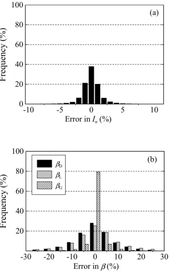
Fig. 6. Percentage frequency distribution of errors in: (a)hourly direct irradiance;(b)turbidity coefficient estimated by each algo-rithm, as pyranometer measurements are affected by a Gaussian random signal.

the original values. These errors exhibit a frequency distribu-tion similar to those shown by global and diffuse irradiances. Figure 6b shows the frequency distribution of the propagated errors in the values of the turbidity coefficient estimated by each algorithm. It may be seen that uncertainties in irradi-ance measurements has a minimal effect on Gueymard’s al-gorithm, with almost 80% of the data associated with relative variations of±2.5%. Dogniaux’s and Louche’s algorithms appear to be more sensitive to those uncertainties, displaying errors of±10% for the 80% of the data.

5.2 Comparison procedure 2

Using SURFRAD and AERONET data from the Bondville station, a comparison between estimated hourly values ofβ by using each broad-band turbidity algorithm and values ofβ derived from AOT records,βsunphot, was undertaken in terms of the statistical tests employed in the previous section. The results are shown in Fig. 7. RMSE and MBE have also been

0.00

0.03

0.06

0.09

0.12

0.15

0.00

0.03

0.06

0.09

0.12

0.15

(a)

MBE = 0.009 (26 %) r2 = 0.58

β

β

0.00

0.03

0.06

0.09

0.12

0.15

0.00

0.03

0.06

0.09

0.12

0.15

(b)

MBE = 0.006 (17 %) r2 = 0.75

β

(

α

ho

t

)

β

0.00

0.03

0.06

0.09

0.12

0.15

0.00

0.03

0.06

0.09

0.12

0.15

(c)

MBE = -0.005 (-14 %) r2 _{= 0.73}

β

β

Fig. 7. Hourly turbidity estimates by using Dogniaux’s (a), Louche’s(b)and Gueymard’s(c)algorithms versus turbidity val-ues derived from sunphotometric measurements at Bondville (βL was calculated employing values ofαobtained from sunphotomet-ric measurements).

0.05 0.10 0.15 0.20 0.25 0.30 0.35 0.40 -0.06

-0.04 -0.02 0.00 0.02

cloudless partly cloudy

β

-

β

k

0 20 40 60 80 100

Frequency

(%

)

and and

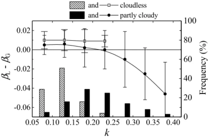
Fig. 8. Average differences β_L(α_sunphot)−βG versus the hourly diffuse fractionkfor both totally cloud-free and partly cloudy sky conditions. Percentage frequency distribution of the diffuse fraction for the two types of sky conditions is also included.

reducing the RMSE around 14% and increasing the coeffi-cient of determination around 17%. Moreover, these latter models provide a lower deviation. In this regard, Gueymard’s algorithm underestimates values ofβ_sunphot around−14%, whereas Louche’s algorithm exhibits the opposite tendency with an overestimation of about 17%.

It is important to note that values ofβLused in this section were calculated using hourly records ofαfrom AERONET measurements, instead of a mean value equal to 1.3. This is the reason for the improvement in Louche’s algorithm per-formance with respect to Dogniaux’s one. Ifαis set to 1.3, the RMSE and MBE values corresponding to Louche’s algo-rithm are 44% and 26%, respectively, whereas ifα=1.7 (the more frequent value ofα_sunphotat Bondville for the selected period), then RMSE=32% and MBE=11%, being r2=0.73 in both cases. The wavelength exponent plays thus an impor-tant role in the performance of Louche’s algorithm, leading to an improvement in the estimates against those by Guey-mard’s algorithm by using a proper value ofα. Moreover, since the statistical results for the performance of the Guey-mard’s algorithm are similar to those for the performance of the Louche’s algorithm using sunphotometric values of the wavelength exponent, it is derived that Gueymard’s algo-rithm is less sensitive to variations in the wavelength expo-nent, even being based on a fixed value of 1.3. Nevertheless, this result should be studied using data from other sites and with different climatic conditions.

On the other hand, cloud interference has a different in-fluence on Louche’s and Gueymard’s algorithms, as it was noted in the previous section. To analyse this influence, we used two hourly data sets: one corresponding to a totally cloud-free sky (the data set filtered by visual inspection – 611 h –), and the other one associated with only partly cloudy conditions. This latter data set was obtained by removing the above totally cloudless data from the data filtered by the ra-diometric criterion given by Eq. (2). Figure 8 shows the av-erage differencesβL(αsunphot)−βGagainst the hourly diffuse

fraction k (defined as the ratio between diffuse and global solar irradiances on a horizontal surface) for both sky con-ditions. In addition, we have included the percentage fre-quency distribution of the diffuse fraction for the two data sets for a better comparison. The diffuse fraction is used as a parameter sensitive to the amount of clouds. Because of the dependency of the hourly diffuse fraction on solar eleva-tion, we used only cases with solar elevation angles above 20◦. It is observed that under totally cloudless conditions, differences are constants for every value ofk. As cloud in-terferences exist, values of both turbidity and diffuse fraction tend to increase. Under these conditions, Louche’s algorithm appears to be less sensitive such as it is derived from the reduction in the differences fork <0.15 with regard to the above constant trend and the notable increasing deviation in the differences as the diffuse fraction is increased.

5.3 Comparison of monthly mean values

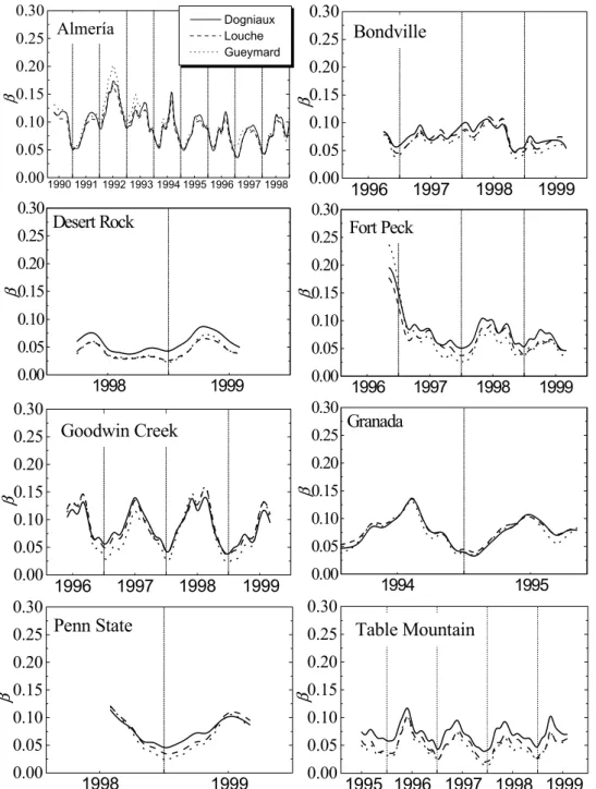
As a final step in our comparative study, we have taken into account that many climatical works deal with long-term vari-ations in atmospheric turbidity (Fox, 1994; Jacovides and Karalis, 1996; Persson, 1999; Devara et al., 2002). In this sense, to examine the long-term differences between each turbidity algorithm, we compared the annual evolution of monthly mean values of β at each location, respectively (Fig. 9). It may be seen that all three algorithms provide trends similar to each other but with small differences. At Almer´ıa, Goodwin Creek, Granada, Penn State and Table Mountain, turbidity presents a seasonal variation with a min-imum for the winter months and a maxmin-imum during the sum-mer due mainly to the increase in water vapor content associ-ated with the higher temperatures. This variation is more ac-centuated at Goodwin Creek. On the other hand, Desert Rock exhibits the lowest turbidity levels along with an almost con-stant trend during the entire year. Bondville and Fort Peck seem to present any annual cycle (at least for the selected months), showing relative maximum and minimum turbidity levels in both summer and winter. It is interesting to note the higher turbidity at Almer´ıa during 1992. This turbidity increase is associated with the eruption of Mount Pinatubo in June 1991, which injected into the stratosphere a large amount of volcanic aerosols (Olmo and Alados-Arboledas, 1995).

6 Conclusions

Atmospheric turbidity is often expressed in terms of the ˚

Angstr¨om turbidity coefficientβ. To calculate coefficientβ in the absence of measurements of spectral solar radiation, different algorithms based on data of broad-band solar radia-tion and meteorological parameters can be used. The aim of this article has focused on the comparison and evaluation of three of these turbidity algorithms.

0.00

0.05

0.10

0.15

0.20

0.25

0.30

1999

1998

1997

1996

1995

Table Mountain

β

0.00 0.05 0.10 0.15 0.20 0.25 0.30

1998 1999

Desert Rock

β

0.00 0.05 0.10 0.15 0.20 0.25 0.30

1995 1994

Granada

β

0.00

0.05

0.10

0.15

0.20

0.25

0.30

1998 1999 1996 1997

Goodwin Creek

β

0.00 0.05 0.10 0.15 0.20 0.25 0.30

1999 1998

1997 1996

Fort Peck

β

0.00

0.05

0.10

0.15

0.20

0.25

0.30

1999

1998

1997

1996

Bondville

β

0.00 0.05 0.10 0.15 0.20 0.25 0.30

Almería

1998 1996 1997

1992 199319941995

1991 1990

Dogniaux Louche Gueymard

β

0.00

0.05

0.10

0.15

0.20

0.25

0.30

Penn State

1999 1998

β

Fig. 9.Annual evolution of monthly mean values of turbidity coefficientβcalculated by each turbidity algorithm at each location.

provides hourly values of precipitable water slightly closer to those computed by Leckner’s and Gueymard’s approaches, if dew point temperature is estimated by Leckner’s formula in-stead of by Magnus’ equation. The three approaches show greater relative differences between each other for low pre-cipitable water, and smaller relative differences between each other for high precipitable water.

Gueymard’s algorithm proved to be the less dependent on precipitable water differences. The pattern of turbidity dif-ferences against precipitable water from Louche’s algorithm was also similar to that by Gueymard’s method, although for precipitable water values less than about 0.5 cm, a large

On the other hand, we have found that Dogniaux’s and Louche’s algorithms provide hourly turbidity estimates closer to each other than by using Gueymard’s method. Moreover, differences on turbidity estimates by Dogniaux’s and Louche’s algorithms were notably reduced by introduc-ing a correction term dependintroduc-ing on precipitable water. Sim-ilarly, random errors in pyranometer measurements have a similar and significant effect on the performance of these lat-ter models. In contrast, the influence of those random un-certainties on turbidity estimates by Gueymard’s method has shown to be of minor importance.

Comparison of estimated turbidity values against turbid-ity values derived from aerosol optical thickness data has shown that the performance of the algorithm by Louche et al. (1987) is significantly improved by settingαto the more frequent hourly value obtained for the location. In such con-ditions, Louche’s and Gueymard’s methods present a similar RMSE of around 34%. In addition, both algorithms exhibit similar absolute deviations with values of 17% and−14% respectively. Settingα to 1.3, the algorithm by Louche et al. (1987) performs similar to that by Dogniaux (1974) with RMSE and MBE values of 48% and 25%. Thus, Guey-mard’s method is the more accurate and reliable, if infor-mation about the wavelength exponent is not available. On the other hand, turbidity algorithms by Dogniaux (1974) and Louche et al. (1987) have shown to be less sensitive to broad-band solar radiation data affected by cloud interference than that by Gueymard and Vignola (1998). Nevertheless, if only a study of annual evolution of the turbidity based on monthly values is to be performed, we have found that all three algo-rithms are suitable for achieving this task.

Acknowledgements. The authors are grateful to SURFRAD’s staff

for providing the solar radiation database. The authors thank B. N. Holben for his effort in establishing and maintaining the AERONET site at Bondville. This work was accomplished thanks to the project (REN/2001)-3890-C02-01/CLI of the Ministerio de Ciencia y Tecnolog´ıa of Spain. The authors thank the valuable suggestions by the anonymous referees.

Topical Editor O. Boucher thanks two referees for their help in evaluating this paper.

References

˚

Angstr¨om, A.: On the atmospheric transmission of sun radiation and in dust in the air, Geogr. Ann., 2, 156–166, 1929.

Augustine, J. A., DeLuisi, J. J., and Long, C. N.: SURFRAD – A national surface radiation budget network for atmospheric re-search, The Bulletin of the American Meteorological Society, 81, 2341–2358, 2000.

ASHRAE: Psychometrics, Handbook of Fundamentals, Refrigerat-ing and Air-ConditionRefrigerat-ing Engineers, American Society of Heat-ing, 1989.

Batlles, F. J., Alados-Arboledas, L., and Olmo, F. J.: On shadow-band correction methods for diffuse irradiance measurements, Solar Energy, 54, 105–114, 1995.

Batlles, F. J., Olmo, F. J., Tovar, J., and Alados-Arboledas, L.: Com-parison of cloudless sky parameterisation of solar irradiance at

various Spanish midlatitude Locations, Theor. Appl. Climatol., 66, 81–93, 2000.

Cachorro, V. E., de Frutos, A. M., and Casanova, J. L.: Determina-tion of the ˚Angstr¨om turbidity parameters, Appl. Opt., 26, 3069– 3076, 1987.

Devara, P. C. S., Maheskumar, R. S., Raj, P. E., Pandithurai, G., and Dani, K. K.: Recent trends in aerosol climatology and air pollution as inferred from multi-year lidar observations over a tropical urban station, Int. J. Climatol., 22, 435–449, 2002. Dogniaux, R.: Representation analytique des composantes du

ray-onnement solaire. Institut Royal de M´et`eorologie de Belgique, S´erie A No. 83, 1974.

Fox, J. D.: Calculated ˚Angstr¨om turbidity coefficients for Fair-banks, Alaska, J. Climate, 7, 1506–1512, 1994.

Gueymard, C., Assessment of the accuracy and computing speed of simplified saturation vapor equations using a new reference dataset, J. Appl. Meteorol., 32, 1294–1300, 1993.

Gueymard, C.: Analysis of monthly atmospheric precipitable water and turbidity in Canada and northern United States. Solar Energy 53, 57–71, 1994.

Gueymard, C.: SMARTS2, A simple model of the atmospheric radiative transfer of sunshine: algorithms and performance as-sessment, Report FSEC-PF-270-95, Florida Solar Energy Cen-ter, Cocos, FL, 1995.

Gueymard, C. and Garrison, J. D.: Critical evaluation of precip-itable water and atmospheric turbidity in Canada using measured hourly solar irradiance. Solar Energy 62, 291–307, 1998. Gueymard, C. and Vignola, F.: Determination of atmospheric

tur-bidity from the diffuse-beam broad-band irradiance ratio. Solar Energy 63, 135–146, 1998.

Holben B. N., Eck, T. F., Slutsker, I. Tanre, D., Buis, J. P., Setzer, A., Vermote, E., Reagan, J. A., Kaufman, Y., Nakajima, T., Lavenu, F., Jankowiak, I., and Smirnov, A.: AERONET – A federated instrument network and data archive for aerosol characterization, Rem. Sens. Environ., 66, 1–16, 1998.

Iqbal, M.: An introduction to solar radiation, Academic Press, Toronto, 1983.

Jacovides, C. P. and Karalis, J. D.: Broad-band turbidity parame-ters and spectral band resolution of solar radiation for the period 1954–1991, in Athens, Greece, Int. J. Climatol. 16, 229–242, 1996.

Janjai, S., Kumharm, W., and Laksanaboonsong, J.: Determination of ˚Angstr¨om’s turbidity coefficient over Thailand, Renew. En-ergy, 28, 1685–1700, 2003.

Kasten, F.: A new table and approximate formula for relative opti-cal air mass, Arch. Meteorol. Geophys. Bioklimatol., Ser. B, 14, 206–223, 1966.

Kasten, F.: A simple parameterization of the pyrheliometric formula for determining the Linke turbidty factor, Meteor. Rundschau. 33, 124–127, 1980.

Kasten, F.: The Linke turbidity factor based on improved values of the integral Rayleigh optical thickness, Solar Energy 56, 239– 244, 1996.

Leckner, B.: The spectral distribution of solar radiation at the earth’s surface – elements of a model, Solar Energy 20, 143–150, 1978.

Li, D. H. W. and Lam, J. C.: A study of atmospheric turbidity for Hong Kong, Renew. Energy 25, 1–13, 2002.

Linke, F.: Transmission Koeffizient und Tr¨ubungsfaktor, Beitr. Phys. Atmos., 10, 91–103, 1922.

ar-tificial neural network models, Agric. For. Met., 107, 279–291, 2001.

Louche, A., Peri, G. and Iqbal, M.: An analysis of the Linke turbid-ity factor, Solar Energy, 37, 393–396, 1986.

Louche, A., Maurel, M., Simonnot, G., Peri, G. and Iqbal, M.: De-termination of ˚Angstr¨om turbidity coefficient from direct total solar irradiance measurements, Solar Energy, 38, 89–96, 1987. M¨achler, M. A.: Parameterization of solar radiation under clear

skies, M. A. Sc. Thesis, University of British Columbia, Van-couver, Canada, 1983.

Marion, W. and George, R.: Calculation of solar radiation using a methodology with worldwide potential, Solar Energy, 71, 275– 283, 2001.

Molineaux, B., Ineichen, P., Delaunay, J. J.: Direct luminous effi-cacy and atmospheric turbidity – improving model performance, Solar Energy, 55, 125–137, 1995.

Mottus, M., Ross, J. and Sulev, M., Experimental studio of ratio of PAR to direct integral solar radiation under cloudless conditions, Agric. For. Met., 109, 161–170, 2001.

Olmo, F. J. and Alados-Arboledas, L.: Pinatubo eruption effects on solar radiation at Almer´ıa (36.83◦N, 2.41◦W), Tellus B, 47, 602–606, 1995.

Pedr´os, R., Utrillas, M. P., Mart´ınez-Lozano, J. A., and Tena, F.: Values of broad band turbidity coefficients in a Mediterranean coastal site, Solar Energy, 66, 11–20, 1999.

Perez, R., Ineichen, P., Seals, R. and Zelenka, A.: Making full use of the clearness index for parameterizing hourly insolation con-ditions, Solar Energy, 45, 111–114, 1990.

Persson, T.: Solar radiation climate in Sweden, Phys. Chem. Earth B. 24, 275–279, 1999.

Pinazo, J. M., Ca˜nada, J., and Bosca, J. V.: A new method to deter-mine ˚Angstr¨om’s turbidity coefficient: Its application for Valen-cia, Solar Energy, 54, 219–226, 1995.

Power, H. C.: Estimating atmospheric turbidity from climate data, Atmos. Env., 35, 125–134, 2001.

Sinha, S., Kumar, S. and Kumar, N.: Energy conservation in high-rise buildings: changes in air conditioning load induced by verti-cal temperature and humidity profile in Delhi, Ener. Conv. Man-agement, 39, 437–440, 1998.

Sh¨uepp, W.: Die Bestimmung der Komponenten der atmo-sph¨arischen Tr¨ubung aus Aktinometer Messungen, Arch. Met. Geoph. Biokl. B, 1, 257–346, 1949.

Unsworth, M. H. and Monteith, J. L.: Aerosol and solar radiation in Britain, Quart. J. Roy. Meteor. Soc., 98, 778–797, 1972. Van Heuklon, T. K.: Estimating atmospheric ozone for solar

radia-tion models, Solar Energy, 22, 63–68, 1979.

Viswanadham, Y.: The relationship between total precipitable water and surface dew point, J. Appl. Meteo., 20, 3–8, 1981.