Social Security E¤ects on Income Distribution: A
Counterfactual Analysis for Brazil
Rodrigo Leandro de Mouray
Brazilian Institute of Economics (IBRE) and EPGE/FGV-RJ
Paulo Sérgio Braga Tafnerz IPEA-RJ
Jaime de Jesus Filhox University of Chicago
Ligia Helena da Cruz Ourives{
EPGE/FGV and Brazilian National Treasury
Abstract
According to Diamond (1977), one of the reasons for the existence of social security systems is that they function as an income redistribution mechanism. There is an extensive literature that tests whether social security systems produce the desired results in developed countries (mainly for the U.S.A.). Nevertheless, there is not an “obvious”consensus about this social security property and there is little evidence for developing countries. In this article, we test this property for the Brazilian Social Security System. In addition, we also look at another question which has not been answered yet in the previous literature. Is the trend of social security systems increasingly progressive or regressive? We conclude that the changes in Brazilian Social Security legislation reduced inequality between 1987 and 1996, but only for the elderly. For the other age groups, there is a stable trend. Results for the period between 1996 and 2006 reveal that the Brazilian system is neutral for all cohorts. Therefore, we found out that social security systems are not an e¤ective mechanism for income redistribution, as predicted by previous studies.
Keywords: Social Security, income distribution, counterfactual distribution. JEL Code: H55, C14, D31.
We are grateful for the comments made by Carlos Eugênio da Costa, Luis Henrique Braido, Marcelo Neri, Ricardo Cavalcanti, from EPGE/FGV; Fernando Holanda Barbosa Filho, from IBRE/FGV; Rafael Souza, Gabriel Hartung and Christiam Gonzáles-Chávez, Ph.D. students from EPGE/FGV; Fábio Gomes from IBMEC-SP; Márcia Marques Carvalho, from UCAM; and all participants of EPGE Economic Research Seminars, XXXV Economic Brazilian National Meeting (Anpec, 2007), LACEA (2008) and NEUDC Conference (2009). Any remaining errors are our own responsibility.
yCorresponding Author. E-mail: [email protected] or [email protected]. A¢liation address (IBRE and EPGE/FGV): 60 Barão de Itambi Street, 8th ‡oor, Botafogo, Rio de Janeiro - RJ, Brazil. Zip Code: 22231-000. Work Phone: +55-21-3799-6482.
1
Introduction
The Brazilian Social Security System follows a pay-as-you-go (PAYG or unfunded) retirement system, like the German, French, Japanese and American systems, in which each generation of workers (current taxpayers) provides …nancial support for the preceding generation’s retirees and pensioners. Due to a peculiar …nancial design, PAYG is vulnerable to some social changes such as demographic and labor market developments. Indeed, there is a consensus that PAYG systems produce an increasing burden on every nation’s budget. Many modern societies have witnessed a worsening situation in their social security systems.
In Brazil, for example, social security de…cit has reached 5% of GDP, one of the highest in the world (Tafner and Giambiagi, 2007). This highlights the fact that the Brazilian system seems to be heading towards insolvency in the future. This has, in fact, been the subject of much public discussion. Proposals for reform of the social security system in Brazil range from a simple invalidation of male/female age di¤erential as a rule for bene…t payments to a complete institutional change in the direction of a funded system, as occurred in the 1980s in Chile.
In this paper, instead of addressing the discussion on what kinds of changes must be made for a better Brazilian system, we think it is important to provide a short discussion of the reasons that justify the existence of public pension systems. Diamond (1977) points out three main justi…cations for a social security: redistribution of income, market failures and paternalism.
Redistribution of Income First, public pensions redistribute income. Ideally, redistribution should be implemented by income taxation on a lifetime basis. Unfortunately, such redistri-bution is rather limited in practice. Annual income taxation is imperfect in terms of income redistribution since the measurement of an individual’s income is restricted to a point in time, without de…ning the needs or capacities of payment, which change throughout the work cycle. Social security, in some countries like Brazil, sets up the bene…t formula based on an average of the highest pre-retirement earnings and not as a function of the wage pro…le throughout the working period. In intragenerational terms, social security works as a complementary mech-anism of redistribution to the income taxation. In intergenerational terms, the increase in the bene…ts in a small fund (as in PAYG) produces a redistribution from the very young to the very old since social security taxes paid by today’s workers and their employers are used to pay the bene…ts for today’s retirees and other bene…ciaries. This kind of redistribution would be appropriate if the oldest generation were poorer on average or if one or more generations experienced long periods of economic recession.
individual’s life cycle. In the case of such risks, social security bene…ts would provide early retirement pensions and disability bene…ts for those who are incapable of working because of illness or disability.
With regard to market failures, we point out two main reasons for a retirement age. First, it is the presence of asymmetric information in the market of an annuity1. Agents with a higher life expectancy would look for this market. So, the price of perpetuity would increase until there is a collapse in the system, driving the market to its own extinction (Rothschild & Stiglitz, 1976; apud, Ferreira, 2007). Government intervenes by de…ning the age at which an eligible retiree receives social security bene…ts after having contributed for some period of time. Secondly, competitive equilibrium in an overlapping generation model might not be Pareto-e¢cient. In the absence of a social security program, people overaccumulate capital over their life cycle, and when they make decisions about savings they do not worry about future generations. So, there is room for government intervention. The dynamic ine¢ciency in the economy would be reduced by the implementation of a mandatory PAYG social security system that would cause a fall in capital stock and an increase in the level of consumption2 .
Paternalism Finally, social security systems force savings. They identify a paternalistic social objective since the utilitarian welfare function depends on ex post utilities. Indeed, government intervention is needed if some individuals are inclined to save less than the amount set aside through payroll taxes. This might occur due to: (i) an incorrect evaluation of current savings according to future needs; (ii) the di¢culty of making savings decisions under uncertainty; (iii) agents’ irrationality as they are future-myopic (strong preference for the present); (iv) the Good Samaritan’s dilemma, when agents save very little because they know society will provide resources at the end of their working years3. Therefore, a pension scheme with forced savings would play an important role in the social security system.
According to the …rst public pension function, public pensions work as a mechanism of income distribution by carrying out public policies in a distributive way. However, at a lower level, as pointed by Tafner (2007), public pensions, just as social insurance, also generate income redistribution in two circumstances: (i) in case of an event (illness, disability or death), a single individual (or his family) receives retirement bene…ts for the rest of his life regardless of how many years he collected social security tax; and (ii) if his life expectancy is su¢ciently high after retirement, he is guaranteed payments that are more than what he paid into the system.
If social security is an advantageous contract for a certain group of people, in particular the poorest ones, then there is a progressive income distribution4. Otherwise, there is a regressive 1In …nance, an annuity is a bond in which periodic payments begin on a …xed date and continue inde…nitely.
Also, annuity can be the right to receive amounts of money regularly over a certain …xed period, in perpetuity, or, especially, over the remaining life or lives of one or more bene…ciaries.
2According to Blanchard & Fischer (1989), any Pareto improvement occurs when the rate of return paid by
the government (which equals the population growth rate) is higher than the interest rate.
3Following Becker & Murphy (1988).
4Progressive means when social security achieves a better income distribution. A social security system is
income distribution5.
There is a wide range of literature that regards social security systems as good policy in-struments for income distribution in industrial countries, especially in the U.S., but there is no clear consensus about that6. In this paper, we evaluate the distributive property of public pensions and try to answer an additional question which has not yet been answered by the literature: “Is the trend of social security systems increasingly progressive or regressive?” Both aspects will be considered for Brazil because: (i) there is little evidence for developing countries which are characterized by high social security expenditure. As already mentioned, in Brazil, the social security de…cit is one of the highest in the world; (ii) Brazil shows a high degree of income inequality7, ranking as the tenth most unequal country in a sample of 126 countries in 2006 (UNDP, 2006).
In order to perform the test, we will deal with taxes and bene…t payments. In a distributive analysis, it is important to consider worker’s social security contribution and bene…t ‡ows
Given the changes in the demographic structure in Brazil, there has been a signi…cant increase in the share of bene…ciaries of the social security system. By controlling some factors, if public pensions have a progressive distributive pattern, we would understand that income inequality might be diminishing. This does not occur in Brazil. For almost two decades, the Gini coe¢cient has been close to 0.60 and has not decayed signi…cantly8.
In order to test the distributive pattern of the system, we shall de…ne the most adequate income measurement. We observe an increase in the social security tax rate (worker and em-ployer) and in the number of bene…ciaries. If we consider that elasticity of tax income is zero, i.e., any increase in the tax rate is not passed on by the …rm as a wage reduction, we believe workers’ gross earnings serve as a measure for social security progressivity. By dealing with in…nite elasticity of tax income, i.e., any increase in the tax rate is fully charged by the …rm as a wage reduction, we consider workers’ net earnings (gross earnings minus contributions). In this case, we choose the latter because it is possible to verify the impact of taxes and bene…t payments, and also because net current income is the most adequate measure in an income inequality analysis.
Furthermore, we observe that lifetime earnings are more appropriate when dealing with the assumption of perfect credit markets, when agents do not have any constraint on borrowing and reallocating wealth from future to present. However, since we consider market failures and, hence, imperfect credit markets, individuals cannot borrow. In general, developing countries tend to face more credit constraints than industrial ones. That is why we use current income9. In Brazil, if a covered worker dies, his or her spouse and children may receive survivors’ bene…ts in a direct (pension) or indirect way (retirement). A broader and more precise analysis
with a higher income.
5Barros & Carvalho (2005) and Tafner (2007) state that the Brazilian social security system is a regressive
one.
6Some of these studies will be commented in the current text.
7Only in recent years has inequality declined. However, not due to the Social Security System, according to
Barros et al. (2007).
8See the preceding footnote.
of the distributive e¤ect of the social security system does not consider individual income but rather family income. If we take the sum of workers’ net earnings of all family members, in per capita terms, we treat the bene…ciary’s family as a bene…ciary and assign that larger families are more dependent upon the social security system.
Still with regard to testing the distributive pattern of the system, in terms of methodology, we look closely at what would happen to per capita family income distribution in Brazil if there were the same share of bene…ciaries and taxpayers as 10 years ago. We had two alternative approaches: (i) a simple regression of wages or (ii) an estimation of densities. The advantage of the latter is the accountability of income distribution. Also, it is possible to calculate various metrics of income inequality and compare them with the real ones. If the social security system has really turned into a more progressive one, we expect to …nd an improvement in income distribution.
Summing up the strategy to test the distributive pattern of the social security system, we …rst describe the sample. After that, we calculate the Gini coe¢cient and the Theil index for wages subtracted by bene…ts. Then, we obtain these same inequality indices for wages added by contributions. By comparing real Gini coe¢cients, we have the joint e¤ect of taxes and bene…t payments on income distribution. Later, we change the distribution of bene…ciaries and taxpayers, controlling for their individual attributes and for geographic characteristics. Also, we estimate a new distribution of per capita family income. At this point, we follow Dinardo, Fortin and Lemieux (1996) to disaggregate counterfactual densities. In addition, we extend the methodology by incorporating contribution ‡ows. Using this general procedure, we achieve a more precise analysis of changes of the progressivity (regressivity) in the social security system.
Graph 1. Beneficiaries/Taxpayers over 18 years old in the Brazilian Population (%)
35.08%
32.56%
34.29%
17.50%
12.81%
18.53%
0% 5% 10% 15% 20% 25% 30% 35% 40%
1987 1996 2006
Share of Taxpayers Share of Beneficiaries
In this analysis, an important assumption is that the changes in social security rules are signaled by the share of bene…ciaries and taxpayers. Graph 1 shows that the share of bene-…ciaries has increased by more than 35% in Brazil: from 12.81% in 1987 to 17.50% in 1996, including an increase of more than 6 basis points in the 10-year period until 2006. At …rst, the share of taxpayers decreased from 35.08% in 1987 to 32.56% in 1996 and increased to 34.29% in 2006. Results for the Gini coe¢cient and the Theil index show that income distribution tended to improve when social security rules were …xed in 1987. This means that the social security system has become more regressive. However, when considering factors such as education, liv-ing and residence standards in 1987, the impact of bene…ts is almost null; that is, those factors explain mainly inequality evolution, reducing the potential e¤ect from social security.
The paper begins in Section 1 by presenting the main functions of the public pension system and then reviews, in Section 2, the literature according to international and Brazilian evidence. Section 3 provides the descriptive statistics and Section 4 explains the methodology used for measuring the distributive pattern of the social security system. Section 5 discusses the results. Section 6 concludes.
2
Literature Review
In what follows, we present a selective review of the American and Brazilian literature related to the distributive aspects of social security.
International Evidence Feldstein (1976) considered bene…ts as part of total family wealth in the U.S. The author suggests that social security systems provide resources within each generation by attempting to give higher returns to lower-wage workers, which reduces their need for fungible wealth accumulation10. For 1962 data, he shows that this kind of wealth inequality is higher than total wealth, which is the progressive distributive pattern of the American system. Evidence is not conclusive, though. Recent studies using an OLG model calibrated to study the transmission of wealth inequality via bequests by Gokhale & Kotliko¤ (2002a, 2002b) and Gokhale et al. (2001) show that social security may greatly increase the inequality in wealth distribution and Gini coe¢cients by 11% (Gokhale & Kotliko¤, 2002a) and 21% (Gokhale & Kotliko¤, 2002b). One of the reasons is that social security transforms bequests into a non-egalitarian force because low-income households rely almost entirely on social security to …nance their retirement consumption, decreasing bequeathable wealth by more than 50%. In contrast, higher-income households have substantial wealth to be passed along to their heirs. The main reason is the American ceiling for social security taxation. As a result, wealthier individuals generally receive larger bene…ts than poorer taxpayers. Liebman (2002) employs a social security microsimulation model. The model simulates the distribution of internal rates of returns, net transfers and lifetime net tax rates from social security that would have been received by individuals born between 1925 and 1929 (age of 73 and 77 in 2002) if they had lived under current social security rules for their entire lives. The author …nds that social security
redistribution is not related to income. Even though social security is thought to be progressive because it redistributes income from the wealthy to the poor, it also transfers income from people with low life expectancies to people with high life expectancies, from men to women, from single workers and from married couples with substantial earnings by the secondary earner11 to one-earner married couples, and from people who work more than 35 years to those who concentrate their earnings in 35 or fewer years. One of the reasons why progressivity of income redistribution in social security system is highly modest is that wealthier individuals generally have higher life expectancies and receive higher bene…ts from their partners. Results point out that 19% of individuals in the largest quintile of lifetime income receive net transfers higher than the average transfers to people in the shortest quintile. Coronado et al. (2000) classify individuals by annual income and the Gini coe¢cients show that the system is highly progressive. Gradually, they control for many factors and recalculate the Gini coe¢cients for every step. According to the potential lifetime income criterion 12,13, they take into consideration that wages above the ceiling are taxed up to the ceiling wage14, adding together the incomes of spouses such that each individual is classi…ed based on the lifetime per capita family income15, incorporate mortality probability16 and increase discount rate from 2 to 4%17. As a result, the progressivity of the system reduces until it becomes regressive.
Brazilian Evidence Afonso & Fernandes (2005) estimate intragenerational and intergenera-tional distributive aspects of the Brazilian social security system by calculating the internal rate of return, which comes from the comparison between bene…t and contribution ‡ows of individu-als in their lifetime. The authors extract bene…ts and infer contributions from the Brazilian National Household Survey, known as PNAD. Contributions also require the distribution of tax payments for di¤erent occupational groups according to the restrictive assumptions about civil servants, own-account and autonomous workers. As a result, the authors imply that the Brazilian social security system is progressive in intragenerational terms (internal rates of return are higher for lower education workers and for those from the Northeast of Brazil, who are also those with lower income per capita) and in intergenerational aspects (internal rates of return decreased from 1980 to 1989 and have been constant since then).
1 1In the U.S., 50% of a living retiree’s bene…t goes to his (her) partner. After his (her) death, the secondary
earner receives the total amount as when he (she) was alive.
1 2The progressivity of social security is reduced because lifetime income classi…es retirees with zero earnings
according to their lifetime revenues. Therefore, agents who work part-time or spend many years of their time out of the labor force are no longer classi…ed as low-income.
1 3The potential lifetime income is the projection of a wage rate for each individual in each period, multiplied
by the total number of hours, resulting in a welfare measure that includes leisure and domestic output instead of job opportunities only.
1 4This taxable maximum was already discussed in the previous paragraph and reduces the progressivity of the
system.
1 5The low-wage spouse is not that poor anymore. This further reduces the progressivity of the system. 1 6As individuals with a higher income live longer, they receive bene…ts for a longer time and, in terms of
measure of current earnings, they tend to receive larger bene…ts. Thus, after these adjustments, the system is too little progressive.
1 7This places more weight on regressive payroll taxes in older years and less weight on progressive bene…t
However, according to the Gini coe¢cient decomposition method, Ferreira (2006) shows that retirements and pensions increase the level of per capita household income inequality in Brazil. Besides, social security gains are the second highest element in the calculation of the Gini coe¢cient, followed immediately by wage earnings. These gains increased from 9.3% in 1981 to 18.8% in 2001 and remained constant. Ho¤mann (2003, 2005) corroborates the …ndings of Ferreira (2006) by using the same Gini coe¢cient decomposition approach. In addition, Ho¤man (2005) applies two other decompositions: Mehran coe¢cient decomposition (more sensitive to changes in the left tail of the distribution) and Piesch coe¢cient decomposition (more sensitive to changes in the right tail of the distribution). Both studies indicate that retirements and pensions contributed to a higher inequality in 1999 (Ho¤mann, 2003) and in the years 2002 to 2004 (Ho¤mann, 2005). Tafner (2007) examines the e¤ect on family poverty using a three-scenario analysis: (i) before bene…t payment; (ii) after bene…t payment; (iii) simulation on the poorest. All scenarios consider the amount of transfers constant. The author concludes that the social security system prevents poverty. Nonetheless, if the social security program had focused on the poorest, there would have been more signi…cant poverty prevention. So, the social security system does not result in a signi…cant inequality reduction and it has not been e¢cient in terms of income distribution. Hence, it shows malfunctions in the income transfer program.
According to Ferreira (2006), the causes for regressivity in the Brazilian social security system are early age retirement; increase in life expectancy, meaning retirees collect bene…ts longer; higher wages for high-income bene…ciaries. All of these factors turn into a worse income distribution. Besides, the causes for a worse de…cit in the Brazilian system are related to the composition and informality of the labor market; ‡exibility in labor contracts (reduction of …xed salary and increase in pro…t sharing agreements, which exclude social security taxation); demo-graphic trends (the number of workers paying into the program continues to decline relative to those receiving bene…ts); legislation (extended bene…ts provided for by the 1988 Constitu-tion). Tafner (2007) also points out that social security net transfers are not only related to income, but also to the occurrence of events. As an example, if wealthier individuals become invalid, they will receive bene…ts for their whole life and will be …nanced by poor people, which illustrates redistribution of wealth from the poor to the wealthy.
Thus, Brazilian evidence is still inconclusive. In this paper, we consider an alternative method to verify the redistributive pattern of the Brazilian social security system.
3
Data and Descriptive Statistics
This paper uses data from the PNAD (Brazilian National Household Survey) to analyze two sets of pairwise years: 1987/1996 and 1996/2006. The ultimate goal is to obtain a more robust and precise evaluation of the distributive characteristics of the social security system18. In fact, 1 8It is important to mention some limitations of the study due to the PNAD data: (i) it is not possible to
there were two important structural breaks in each set: (i) 1987/1996: The Constitution of 1988 altered social security rules; and (ii) 1996/2006: The Social Security Reform in 2003 altered the rules for civil servants.
The analysis requires the application of …lters. First, all observations with individuals under the age of 18 years were excluded from the samples. Anyway, this represents a small percentage of bene…ciaries19, only 2% of the total. Second, we exclude all households in which all members declared receiving no income20. So, only individuals aged over 18 years and reporting some income were kept in the sample. The descriptive statistics of the sample is shown below.
We notice that the share of bene…ciaries has increased enormously up to 35% (Graph 1 in the Introduction). Table 1 in Appendix A indicates that the number of bene…ciaries also increased: from 10.10 millions in 1987 to 16.13 millions in 1996 and 22.95 millions in 2006. Pensions showed a huge increment in terms of relative participation: from 24.48% in 1986 to 36.10% in 2006. Elderly people (over 58 years old) constitute a high share of bene…ciaries that has been increasing over the years.
In terms of share of taxpayers, there has been a recovery in the last decade after an initial slowdown. The number of taxpayers has almost doubled: from 27.5 million in 1987 to 41.78 million in 2006. Ordinary workers are the ones who pay more. In general, since 1996, the share of contributions has raised to a high degree especially as a result of the Social Security Reform in 2003, which has enlarged the number of contributions by incorporating retired civil servants. We have calculated the Gini coe¢cient and Theil index for the whole …ltered sample and for age groups. We subtracted bene…ts and added tax payments, separately and jointly. Table 2 shows the estimations for these coe¢cients as gross samples with no controls. By comparing (1), bene…ts induce a reduction in net family income per capita inequality for individuals aged over 18 years. That is, the social security system is a progressive system, in terms of bene…ts. Moreover, the system has become more and more progressive as column “(1)/Factual” shows absolute gains over the years. Also, by comparing (2), contributions have no distributive e¤ect. Jointly, taxes and bene…t payments have a progressive e¤ect on inequality, in level and monotonic terms. Note that the reduction in the inequality level is up to 9.5% for the Gini coe¢cient and 19.5% for the Theil index. Even according to age groups, the bene…t e¤ect is progressive and increases with age. For early ages, there is a relatively small gain. Also, the tax payment e¤ect is negligible.
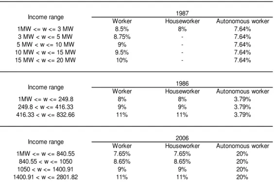
informality once information about the labor market is not available. Afonso & Fernandes (2005) had the same limitation. Another element is the inexistence of questions about tax values. Following Afonso & Fernandes (2005)’s strategy, we obtained the following from PNAD data: values for earnings, an indicator function for taxpayer (or not) in every occupation, type of occupation in productive activity (ordinary worker, civil servant, houseworker or autonomous worker). Then, social security taxes and rates were obtained for every working group from each occupation’s earnings. In Appendix B, in Table 9, we show a brief description of legislation history and rates applied.
1 9We consider bene…ciaries those who receive a positive income from retirement, pension or nonretirement
allowance. In earlier PNAD data, there is no question about whether the individual is a retiree/pensioner or if he (she) receives any kind of nonretirement allowance. The only question was about what the individual had done during the week. A busy retiree would have answered that he (she) worked as usual. This means a biased share of bene…ciaries in earlier pools.
For individuals under 47 years old, the joint e¤ect (contribution and bene…t) of progressivity increase is smaller (see column “Factual/(3)”). Nonetheless, for individuals aged over 48 years, taxes and bene…t payments imply progressivity in income distribution, and changes in social security rules have turned the system into a more progressive one. In the U.S., Feldstein (1976) and Coronado et al (2000) reached similar evidence when they also did not control for several factors.
As mentioned before, the use of controls is highly required to separate the real e¤ect of an improvement of the social security system. To achieve that, we consider kernel density estimation.
4
Methodology
Following Dinardo, Fortin and Lemieux (1996, hereinafter DFL), we use weighted kernel density estimators21. The kernel density estimatefbhof a univariate densityf based on a random sample
of wages 22 fWigni=1of sizen, with weightsf ig
n i=1,
P
i i = 1 is:
b
fh= n P i=1
i hK
w Wi
h ;
wherehis the smoothing parameter (or bandwidth) andK(:)is the kernel function. According to Silverman (1986), there are few e¢ciency di¤erences (in terms of the norm of integrated mean square error) among di¤erent kernels. So, the kernel function used is Gaussian kernel as in DFL. As bandwidth selector, we use Silverman’s rule of thumb (1986), based on the standard deviation and interquantile range:
h= 0:9 minf w; Rw=1:34g
n1=5
where w is the standard deviation of the sample and Rw is its interquantile range. In all
nonparametric estimates, the domain of estimated densities is the logarithm of income, whose support is de…ned on the interval [0.01,14], with steps of 0.01, including the whole income mass.
4.1 Estimation of Counterfactual Densities
The procedure in DFL allows for the analysis of the whole distribution. Our estimation of counterfactual densities intends to answer the following question: “what would the density of wages have been in 1996 if the share of bene…ciaries-taxpayers had remained at its 1987 level”23. 2 1DFL adapted these estimators, which were originally introduced by Rosenblatt (1956) and Parzen (1962). 2 2Wages refer to logarithm ofper capitanet family income.
2 3This counterfactual approach is subject to Lucas critique. That is, individuals could change their behavior
if a change in government policy is expected, such as an increase in bene…ts. The technique does not incorporate adjustments and expectations from individuals. For instance, we could mention a change in the decision of a woman who receives a pension and could separate from her husband because she used to be battered.
Consider each observation as a vector (w; z; t), where w is the logarithm of the sum of net earnings of all family members in per capita terms (continuous variable), z are the individual attributes (dummy for bene…ciaries and taxpayers, dummies for schooling years, age, race and marital status, dummy for whether the individual is head of family, interaction dummy for head of family and sex, total hours of work, place of residence [urban or rural] and dummies for the states where the individual lives) and a date t, which takes only two values in the comparisons and includes years 1987, 1996 and 2006. The subvector z is divided into three parts: z = (b; c; x), where b is a dummy variable for bene…ciaries, c is a dummy variable for taxpayers and x are all other factors. This division (into b,c and x) is due to the focus of our paper on the social security structure, denoted by variables b and c, which have been altered over the last years. Consider the joint distribution of wages, individual attributes and dates,
F(w; b; c; x; t). This distribution of wages and attributes at one point in time is the conditional distributionF(w; b; c; xjt). The density of wages at one point in time, ft(w), can be written as
the integral of the density of wages conditional on a set of individual attributes and on a date
twjb;c;x,f wjb; c; x; twjb;c;x , over the distribution of individual attributesF(zjtz)at date tz:
ft(w) = Z
x2 x
Z
b2 b
Z
c2 c
dF(w; b; c; xjtw;b;c;:x=t)
=
Z
x2 x
Z
b2 b
Z
c2 c
f wjb; c; x; twjb;c;x=t dF(bjc; x; tbjc;x =t)dF(cjx; tcjx =t)dF(xjtx=t)
= f w;twjb;c;x=t; tbjc;x=t; tcjx=t; tx =t ;
where x; b; cis the domain of de…nition of the individual attributes. The notationtw;b;c;x =t
represents the values of wages, share of bene…ciaries, share of taxpayers and all other individual attributes at datet. For example,f w;twjb;c;x = 96; tbjc;x = 96; tcjx= 96; tx = 96 represents the
actual density of wages in 1996. In the case of f w;twjb;c;x= 96; tbjc;x = 87; tcjx= 96; tx= 96 ,
it represents the counterfactual density of wages in 1996 ifonlythe bene…ts (variableb) had re-mained at their 1987 level, while all other attributes had been according to the wage schedule ob-served in 1996. Under the assumption that the 1996 structure of wages24,f wjb; c; x; twjb;c;x = 96 ;
does not depend on the 1987 distribution of attributes,dF(bjc; x; tbjc;x = 87), we may write the counterfactual densityf w;twjb;c;x= 96; tbjc;x = 87; tcjx = 96; tx= 96 , in which onlythe share
of bene…ciaries is constant at the 1987 level, but the other attributes are at the 1996 level, is25:
f w;twjb;c;x = 96; tbjc;x= 87; tcjx= 96; tx = 96 =
" R R R
f wjb; c; x; twjb;c;x = 96 dF(bjc; x; tbjc;x= 87) dF(cjx; tcjx = 96)dF(xjtx= 96)
#
=
Z Z Z
f wjb; c; x; twjb;c;x= 96 bjc;x(b; c; x)dF(bjc; x; tbjc;x = 96)dF(cjx; tcjx= 96)dF(xjtx = 96) ;
(1) 2 4In the explanation of the methodology, we always used year 1996, with the attributes set at the level of 1987,
for simplicity. But, we made inferences by also comparing a diferent pair of years (1996/2006).
where, bjc;x(b; c; x)is the reweighting function de…ned as:
bjc;x(b; c; x) dF(bjc; x; tbjc;x = 87)=dF(bjc; x; tbjc;x = 96)
= bPr b= 1jc; x; tbjc;x = 87
Pr(b= 1jc; x; tbjc;x= 96) + (1 b)
Pr b= 0jc; x; tbjc;x = 87
Pr(b= 0jc; x; tbjc;x= 96); (2)
where the last part in equation (2) is obtained when b is a dummy such as dF(bjc; x; tbjc;x) = bPr b= 1jc; x; tbjc;x + (1 b) Pr b= 0jc; x; tbjc;x . Note that this counterfactual density is identical to the factual density (1996) except for the function bjc;x(b; c; x)26. So, the estimation of counterfactual densities is simply the estimation of the reweighting function. Thus, the counterfactual density kernel estimator is:
b
f w;twjb;c;x = 96; tbjc;x = 87; tcjx= 96; tx= 96 = P i2S96
i
h bbjc;x(b; c; x)K
w Wi
h : (3)
The di¤erence between the actual 1996 density and this hypothetical density represents the e¤ect of changes on the distribution of bene…ciaries, ceteris paribus all other factors. A way to estimate the reweighting function of equation (2) is by estimating a probit model for each year separately27, that is, to estimate:
Pr(b= 1jc; x; tbjc;x =t) = 1 ( 0tG(c; x)); (4)
where (:) is a normal distribution function and G(:) is a function of other attributes.
The counterfactual distribution in case b and c would have remained at the 1987 level (if social security system had remained unchanged by the Constitution of 1988), as shown:
f w;twjb;c;x = 96; tbjc;x= 87; tcjx= 87; tx = 96 =
" R R R
f wjb; c; x; twjb;c;x = 96 dF(bjc; x; tbjc;x= 87) dF(cjx; tcjx = 87)dF(xjtx= 96)
#
=
" R R R
f wjb; c; x; twjb;c;x= 96 bjc;x(b; c; x)dF(bjc; x; tbjc;x= 96)
cjx(c; x)dF(cjx; tcjx = 96)dF(xjtx = 96)
#
;
where cjx(c; x) =dF(cjx; tcjx = 87)=dF(cjx; tcjx = 96). The same way as in (4), it is possible
to estimate cjx(c; x) through a probit model with a dummy variable c and the same set of regressors:
Pr(c= 1jc; x; tcjx=t) = 1 ( 0tH(x)); (5)
2 6Note that the 1996 factual density could have been written as:
ft(w) = f w; twjb;c;x= 96; tcjx= 96; tx= 96
=
Z Z Z
f wjb; c; x; twjb;c;x= 96 dF bjc; x; tbjc;x= 96 dF bjc; x; tcjx= 96 dF(xjtx= 96)
The only di¤erence in relation to equation (1) is the insertion of reweighting function bjc;x(b; c; x).
2 7More speci…cally, we estimate this probit model for 1987 and 1996 separately. After that, we insert the
adjusted probabilitycPr(b= 1jx; tbjx=t), and we expand it for the whole sample. Then, when we use the 1996
data, we will havePr(cb= 1jx96; tbjx= 96)andcPr(b= 1jx96; tbjx= 87), i.e., the probability of being a bene…ciary
Finally, by altering b; c and x, the counterfactual density is:
f w;twjb;c;x = 96; tbjc;x= 87; tcjx= 87; tx = 87 =
" R R R
f wjb; c; x; twjb;c;x = 96 dF(bjc; x; tbjc;x= 87)
dF(cjx; tcjx = 87)dF(xjtx= 87)
#
=
" R R R
f wjb; c; x; twjb;c;x= 96 bjc;x(b; c; x)dF(bjc; x; tbjc;x= 96)
cjx(c; x)dF(cjx; tcjx = 96) x(x)dF(xjtx = 96)
#
;
where x(x) = dF(xjtx = 87)=dF(xjtx = 96). Applying the Bayes’rule, this ratio can be
written as:
x(x) =
Pr(tb = 87jx)
Pr(tb = 96jx)
Pr(tb = 96)
Pr(tb = 87) :
So, to infer the …rst ratio, we simply estimate a probit of the year against variablexand for the second ratio we calculate the proportion of observations in each year. We can now estimate the counterfactual densities by operating:
b
f w;twjb;c;x = 96; tbjc;x= 87; tcjx= 96; tx = 96 = P i2S96
i
h bbjc;x(b; c; x)K
w Wi
h ;
b
f w;twjb;c;x = 96; tbjc;x= 87; tcjx= 87; tx = 96 = P i2S96
i
h bbjc;x(b; c; x)bcjx(c; x)K
w Wi
h ;
b
f w;twjb;c;x = 96; tbjc;x= 87; tcjx= 87; tx = 87 = P i2S96
i
h bbjc;x(b; c; x)bcjx(c; x)bx(x)K
w Wi
h ;
that is, we multiply the new weights by the weight extracted from PNAD, according to each density. Thus, the change in variables for the 1987 level will be in the following order: bene…ts, contributions and other factors. This decomposition is callednormal decomposition28, whose results will be shown in the following section.
Before that, it is important to highlight that the estimation of densities was made for the logarithm of income. To do so, we need to obtain the distributions of income level. It is a simple procedure. Consider the wage variable as v = exp(w), such that the distribution function is
Fv(v). We have the following transformation:
Fv(v) = Pr (v v) = Pr (exp (w) v) = Pr (w ln (v)) =Fw(ln (v)):
By di¤erentiating it, we have the density function:
fv(v) =
fw(ln (v))
v =
fw(w)
exp (w):
that is, simply take the estimated density for the logarithm of income and divide it by the exponential of the domain. From this density, it is possible to infer many inequality metrics.
5
Results
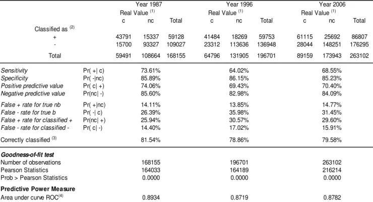
First, probit models (4) and (5) were well adjusted as shown in Tables 4 and 5. The estimated probits for variables b and c, as dependent variables, had a high percentage of correct classi-…cation (around 90 and 80%, respectively), as well as high Pearson’s statistics and predictive power measure for the estimated models in a general sample (individuals aged over 18 years).
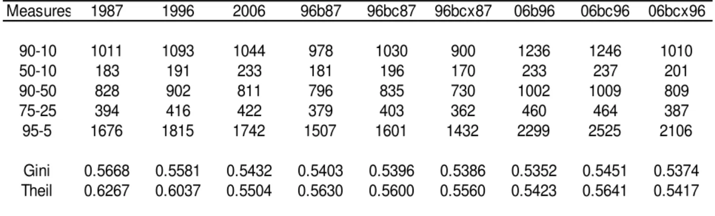
From the estimation of densities for counterfactual considerations, Table 5 shows the meas-ures of di¤erentials between percentiles and inequality indicators. By comparing 1996/2006 factual with 1986/1996 counterfactual densities of bene…ts (96b87, 06b96), we notice there was a decrease in the di¤erentials, that is, the increase in the share of bene…ciaries raised the wage gap between the wealthy and the poor. On the other hand, the e¤ect of contributions is a re-duction in the gap. The Gini coe¢cient and Theil index corroborate in a more accurate way the distributive pattern of the social security system. The joint e¤ect of taxes and bene…t payments implies worsening of inequality as we compare 96bc87 to 1996, where the Gini coe¢cient (Theil index) increases from 0.5396 (0.5600) to 0.5581 (0.6037).
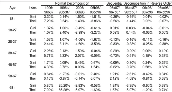
Table 8 summarizes the percentage change of the Gini coe¢cient and Theil index of factual and counterfactual densities. In the sample of individuals over 18 years old, the e¤ect of bene…ts raises the Gini coe¢cient (Theil index) coe¢cient by 3.30% (7.23%) when comparing 1996 to 96b87 (the percentage is the ratio of factual and counterfactual densities) and raisesit by 1.5% (1.49%) when comparing 2006 to 06b96. Since we have maintained the share of bene…ciaries constant in the base year, we consider the e¤ect of also …xing the share of taxpayers in the base year (by comparing, as an example, 96b87 to 96bc87 densities). Thus, the e¤ect of contributions is almost none from 1987 to 1996 (0.14% [Gini] and 0.54% [Theil]) and progressive from 1996 to 2006 (-1.81% [Gini] and -3.86% [Theil]). By maintaining all social security rules constant in the base year (b and c at the 1987 level), the e¤ect of other factors29 is almost none from 1986 to 1996 (0.18% [Gini] and 0.71% [Theil]) and regressive for the next period (1.42% [Gini] and 4.14% [Theil]).
The estimations of counterfactual densities corroborate the distributive pattern of income distribution of the Brazilian social security system in the last decades. Both components of the social security structure (taxes and bene…t payments) provide a raise in inequality30 between 1987 and 1996. It means the system has become more regressive. In the last decade (1996-2006), both e¤ects are in the opposite direction and hence the joint e¤ect is almost none for inequality. That is, the system has not featured any trend towards increasing progressivity/regressivity; it has remained almost unchanged.
5.1 Sequential Decomposition in Reverse Order
So far, we have evaluated the e¤ect of taxes and bene…t payments followed by the e¤ect of other attributes. However, the results can be altered if we have a reverse order of the e¤ects. To perform the sequential decomposition in reverse order, that is, alteringx,c andb, respectively, we apply the procedure described in the previous section, but in reverse order, following DFL (we have to estimate xjc;b(x; c; b), cjb(c; b) and b(b)). Thus:
b(b) =
dF(bjtb = 87) dF(bjtb = 96)
Bayes’ Rule
= Pr(tb = 87jb) Pr(tb = 96jb)
Pr(tb= 96)
Pr(tb= 87)
2 9The percentage was omitted, but can be easily veri…ed by dividing 96bc87 by 96bcx87 and 06bc96 by 06bcx96. 3 0The e¤ect can be approximately measured as the sum of percentages of Table 8. For example, under normal
can be estimated as x(x), replacingx withb
.
The term cjb(b; c)de…ned as:cjb(c; b) dF(cjb; tcjb = 87)=dF(cjb; tcjb = 96)
= cPr c= 1jb; tcjb = 87
Pr(c= 1jb; tcjb = 96) + (1 c)
Pr c= 0jb; tcjb = 87 Pr(c= 0jb; tcjb = 96);
is estimated analogously as in (4), ) with a probit model, dependent variable c and independ-ent variable b. To estimate xjc;b(x; c; b), we know that: F(b; c; x) = F(bjc; x)F(cjx)F(x) =
F(xjc; b)F(cjb)F(b). By applying the Bayes’rule, we have:
bxjc;b(x; c; b) = bbjc;x(b; c; x)bcjx(c; x)bx(x)
bcjb(c; b)bb(b)
;
where the numerator and bb(b)have already been calculated during the normal decomposition
and the term bcjb(c; b)is obtained as above.
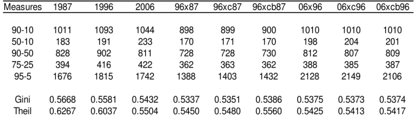
Reverse decomposition results Table 6 shows the results for the sequential decomposition in reverse order and Table 8 displays the percentage change in the right column. If we consider the e¤ect of maintaining other factors31 constant at the base year level, we …nd a higher increase in the Gini coe¢cient (Theil index) of 4.58% (10.77%) from 1987 to 1996 and a slightly lower raise in the next decade (1.06% [Gini] and 1.46% [Theil]). Still considering the whole sample (individuals aged over 18 years), taxes and bene…t payments have little e¤ect on the two decades as all attributes are constant at the base year level.
And by keeping other attributes, share of bene…ciaries and taxpayers constant at the base year level, the total e¤ect is the deterioration in income inequality. The Gini coe¢cient (Theil index) increased 3.63% (8.57%) from 1986 to 1996 (when comparing 1996 to 96xcb87) and 1.08% (1.61%) in the next 10 years (when comparing 2006 to 06xcb96). So, changes in individual attributes such as education, marital status, race, age group, working hours and geographical variables, have shown an increasing regressivity in the distribution of family income per capita. From normal decomposition to sequential decomposition in reverse order, the social security system seems to be less regressive, especially when comparing the 1987-1996 period. This results from the conditioning of other factors (variables x), which explain most of the evolution of inequality over the years and reduce the potential e¤ect of social security on the distribution. Some variability in b and c is due to the variability of x. As an example, the demographic changes (variable age in x) imply a higher increase in the number of bene…ciaries. If we keep demographic changes at the 1987 level, we raise the proportion of young people and reduce some reasonable e¤ect of bene…ts, since young people have a lower probability to receive bene…ts as the probability of being a taxpayer has changed too little in the period (Table 1).
3 1The e¤ect is obtained, for example, by the ratio of the Gini coe¢cient (Theil index) from 1996 and 96x87
5.2 Analysis of age structure
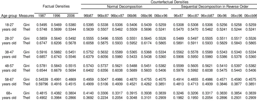
To consider the intergenerational distributive pattern of the social security system, we reestimate factual and counterfactual densities by age groups. Table 7 summarizes the results of the Gini/Theil coe¢cients and Table 8, the percentage change for both decompositions.
The joint e¤ect of taxes and bene…t payments from 1987 to 1996 (sum of the percentages of 1996/96b87 and 96b/96bc87 ratios) indicates an increase in regressivity for all ages (except for the age of 58-67 years), especially for the oldest (over 68 years old). Nonetheless, in regard to years 1996-2006, there has been a transition in the trend (for the sum of percentages of 2006/06b96 and 06b96/06bc96 ratios) for the youngest group (18-37) and the oldest group (68+). The 38-57-year-old cohort continues featuring bad inequality, while the 58-67-year-old cohort shows a reverse trend in relation to the last decade. The same occurs for the e¤ect of contributions, except for the 58-67-year-old cohort. Thus, individuals over 68 years old in 2006 were in a better position than the ones in 1996, who were worse than individuals in 1986, due to the changes in social security rules. The same reasoning applies to young people.
We also applied the analysis for sequential decomposition in reverse order for age structure (right columns in Table 8). The distributive e¤ects of changes in social security rules, given the change in other factors, tend to be relatively small for the 48-57-year-old cohort. For the 58-67-year-old cohort, the total e¤ect (bene…ts and tax payments) increased progressivity for the 1987-1996 period and goes from increasing regressivity to stable for the 1996-2006 period. For individuals aged over 68 years, the total e¤ect (bene…ts and contributions) increased progressiv-ity for the 1987-1996 period and goes from increasing regressivprogressiv-ity to stable for the 1996-2006 period. The Gini coe¢cient (Theil index) decreased up to 2.10% (3.41%) for this cohort in the 1987-1996 analysis, but the e¤ect was less than 0.5% for the last decade.
In general, even when the e¤ect of bene…ts and contributions was conditioned on variable x, there was an improvement in inequality for the oldest cohorts from 1987 to 1996, but this trend disappeared from 1996 to 2006.
5.3 Comments
Ferreira (2006) and also other authors have already pointed out some of the reasons for the increasing regressivity in the Brazilian social security system under normal decomposition, such as early age retirement, higher life expectancy, and higher wages for high-income bene…ciaries. Gokhale & Kotliko¤ (2002a and 2002b), Gohale et al. (2001) and Tafner & Giambiagi (2007) highlight the contribution ceiling.
Table 9 displays the ceiling for contributions: it used to be 20 times the regional minimum wage until 1984. After that, it became 20 times the federal minimum wage. In 1989, the ceiling decreased to 10 times the minimum wage and nowadays it is around 8 times the minimum wage (see footnote in the table). So, high-income individuals pay proportionally less. Since 1989, a higher number of high-income individuals has been paying less. This might have contributed to the increasing regressivity in the system by the end of the 1980s and half of the 1990s.
dis-tributive e¤ects. According to Liebman (2002) and Tafner & Giambiagi (2007), social security implies redistribution that is not related only to income (that is, income redistribution from the wealthy to the poor), as emphasized by normal decomposition analysis. Under the decom-position in reverse order, social security also implies redistribution among people with di¤erent individual attributes. Therefore, the joint e¤ect of these attributes (variable x) implies stability of the distributive e¤ects over the years. For example, income transfer from individuals with less schooling years to those with more education, from non-whites to whites, from single to married couples, and from rural to urban residences has not increased.
On the one hand, normal decomposition can be interpreted as follows: in terms of inequality, individuals who earn according to the 1996 (2006) wage level with individual attributes (educa-tion, working hours, age, etc) compatible with year 1996 (2006) and who live according to the 1996 (2006) social security rules are worse (equal) when compared to the same individuals living according to the 1987 (1996) social security rules. On the other hand, under the decomposition in reverse order, individuals who earn according to the 1996 (2006) wage level with individual attributes compatible with year 1987 (1996) and who live according to the 1987 (1996) wage level are stable when compared to the same individuals living according to the 1996 (2006) social security rules
Therefore, our preferred estimates are those of the sequential decomposition in reverse order. From normal decomposition to sequential decomposition in reverse order, the social security system seems to be less regressive, especially when comparing the 1987-1996 period. This results from the conditioning of other factors (variables x), which explain the evolution of inequality over the years and reduce the potential e¤ect of social security on the distribution.
Our conclusion is that the Brazilian social security system implies income distribution that is not related only to income, but also to individual attributes. Further research is needed to verify the most in‡uential causes for the increase in the regressivity of the Brazilian social security system.
6
Concluding Remarks
In this paper, we conclude that the Brazilian social security system has a distributive pattern throughout the period of analysis. Only when taxes and bene…t payments were kept constant at the 1987 level did the system become less progressive. In other words, between 1987 and 1996, the changes in retirement rules (captured by the share of bene…ciaries and taxpayers) contributed to increasing the regressivity of the system. However, when the variables (x) related to individuals and to geographical attributes were kept constant at the base year level, the e¤ect of taxes and bene…t payments became stable for the whole sample. In the last decade, from 1996 to 2006, both decompositions showed a trend towards stability.
For this reason, in opposition to some of the previous literature, the results reveal that retirement systems are not a good policy instrument for income redistribution. Therefore, in spite of the fact that PAYG systems, such as the Brazilian one, contribute to reducing poverty levels, there seems to be a growing need for reforms in countries that adopt this system. In Brazil, the Social Security Reform was partly accomplished in 2003, by reducing and postponing the insolvency trap. Besides, social security systems tend to be ine¢cient. De Carvalho Filho (2008) showed one of these ine¢ciency dimensions when studying the establishment of new retirement bene…ts (or increasing those which already exist) and the reduction of the minimum age for retirement, in 1991, for Brazilian rural workers. This study concluded that the 1991 Law had a negative impact on the decision to participate in the labor market, because it increased the probability of not working, and it reduced the total number of working hours.
In conclusion, the ample evidence presented in this paper suggests that the Brazilian social security system is not suitable for producing a higher level of equity. In other words, PAYG systems are not adequate policy tools for income redistribution, as some of the literature sug-gests. In view of the results we conclude that the Brazilian PAYG system has a high cost for the Brazilian economy.
References
[1] Afonso, L. E., R. Fernandes (2005). Uma Estimativa dos Aspectos Distributivos da Pre-vidência Social no Brasil.Revista Brasileira de Economia, 59(3): 295-334.
[2] Barros, R. P. de, M. Carvalho (2005). Salário mínimo e distribuição de renda. Rio de Janeiro: IPEA. (Seminários Dimac, n. 196).
[3] Barros, R. P. de, M. Carvalho, S. Franco, R. Mendonça (2007). A importância da queda recente da desigualdade na redução da pobreza. Texto para discussão, n. 1256, Rio de Janeiro: IPEA.
[4] Becker, G. S., K. M. Murphy (1988). The Family and the State. Journal of Law and Economics, 31(1): 1-18.
[5] Blanchard, O. J., S. Fischer (1989).Lectures on Macroeconomics. Cambridge: MIT Press. [6] Coronado, J. L., D. Fullerton, T. Glass (2000). The Progressivity of Social Security. NBER
Working Paper, 7520.
[7] De Carvalho Filho, Irineu Evangelista (2008). Old-age bene…ts and retirement decisions of rural elderly in Brazil. Journal of Development Economics, Forthcoming.
[8] Diamond, P. A. (1977). A framework for social security analysis. Journal of Public Eco-nomics, 8(3): 275-298.
[9] Dinardo, J. N. M. Fortin T. Lemieux (1996). Labor Market Institutions and the Distribution of Wages, 1973-1992: A Semi-parametric Approach. Econometrica, 64(5):1001-1044. [10] Feldstein, M. (1976). Social Security and the Distribution of Wealth.Journal of the
[11] Ferreira, C. R. (2006). Aposentadorias e Distribuição da Renda no Brasil: uma nota sobre o período 1981 a 2001.Revista Brasileira de Economia, 60(3): 247-260.
[12] Ferreira, S. G. (2007). Sistemas Previdenciários no Mundo: Sem ”Almoço Grátis”. In: Tafner, P. and F. Giambiagi (ed.), Previdência no Brasil: debates, dilemas e escolhas. Rio de Janeiro: IPEA, cap.2: .65-93.
[13] Giambiagi, F., K. Beltrão, J. Mendonça, V. Ardeo (2004). Diagnóstico da previdência social no Brasil: o que foi feito e o que falta reformar? Pesquisa e Planejamento Econômico, 34(3).
[14] Gokhale, J., L. J. Kotliko¤ (2002a). Simulating the Transmission of Wealth Inequality.The American Economic Review - Papers and Proceedings, 92(2): 265-269.
[15] —————. (2002b). The Impact of Social Security and Other Factors on the Distribution of Wealth. In: Feldstein, M. and J. B. Liebman (ed.), The Distributional Aspects of So-cial Security and SoSo-cial Security Reform. Chicago: University of Chicago Press, chap.3: 85-114.
[16] Gokhale, J., L. J. Kotliko¤, J. Sefton, M. Weale (2001). Simulating the transmission of wealth inequality via bequests.Journal of Public Economics, 79: 93-128.
[17] Ho¤mann, R. (2003). Inequality in Brazil: The Contribution of Pensions.Revista Brasileira de Economia, 57(4): 755-773.
[18] —————. (2005). As transferências não são a causa principal da redução na desigualdade.
Econômica, 7(1): 77-95.
[19] Liebman, J. B. (2002). Redistribution in the Current U.S. Social Security System. In: Feldstein, M. e J. B. Liebman (ed.), The Distributional Aspects of Social Security and Social Security Reform. Chicago: University of Chicago Press, chap.1: 11-48.
[20] Oaxaca, R. (1973). Male-Female Wage Di¤erentials in Urban Labor Markets.International Economic Review, 14: 693-709.
[21] Parzen, E. (1962). On Estimation of a Probability Density Function and Mode.The Annals of Mathematical Statistics, (33): 1065-1076.
[22] Rosenblatt, M. (1956). Remarks on Some Non-parametric Estimates of a Density Function.
The Annals of Mathematical Statistics, (27): 832-837.
[23] Rothschild, M., J. Stiglitz (1976). Equilibrium in Competitive Insurance Market.Quarterly Journal of Economics, 90: 630-649.
[24] Saboia, J. L. M. (1984). Evolução histórica do salário mínimo no Brasil: Fixação, valor real e diferenciação regional. PNPE. Série Fac-Símile 15.
[25] Silverman, B. (1986).Density Estimation for Statistics and Data Analysis. London: Chap-man & Hall.
[27] Tafner, P., F. Giambiagi (2007). Introdução. In: Tafner, P. and F. Giambiagi (ed.), Previd-ência no Brasil: debates, dilemas e escolhas. Rio de Janeiro: Ipea, Introdução: 11-25. [28] UNDP (United Nations Development Programme) (2006). Human Development Report
7
Appendix A
Table 1. Characteristics of Beneficiaries and Taxpayers in the Brazilian Social Security System
Statistics Statistics
1987 1996 2006 1987 1996 2006
Number of beneficiaries (in millions) Number of contributors (in millions)
Retirement 7.59 11.18 14.66 Worker 21.77 21.44 31.67
Pension 2.47 4.95 8.28 Civil Servant 2.20 4.21 5.50
Nonretirement allowance 0.04 0.01 0.01 Houseworker 0.67 1.18 1.86
Autonomous worker 2.86 2.78 2.74
Total 10.10 16.13 22.95 Total 27.50 29.61 41.78
Share of each type of benefit Share of each type of taxpayer
Retirement 75.17% 69.31% 63.86% Worker 79.16% 72.41% 75.81%
Pension 24.48% 30.66% 36.10% Civil Servant 8.01% 14.21% 13.17%
Nonretirement allowance 0.35% 0.03% 0.04% Houseworker 2.43% 3.97% 4.46%
Autonomous worker 10.40% 9.40% 6.56%
Share of beneficiaries within each age group
Share of taxpayers within each age group
18-27 years old 0.58% 1.47% 2.40% 18-27 years old 36.39% 32.08% 34.50%
28-37 years old 2.04% 3.22% 4.03% 28-37 years old 45.31% 42.21% 44.83%
38-47 years old 23.39% 17.84% 35.61% 38-47 years old 41.56% 42.42% 44.06%
48-57 years old 19.52% 24.00% 20.56% 48-57 years old 30.29% 30.02% 35.05%
58-67 years old 44.24% 60.44% 60.73% 58-67 years old 16.28% 14.15% 14.69%
68+ years old 83.45% 88.43% 87.67% 68+ years old 2.98% 2.56% 2.20%
Source: PNAD/IBGE
Note:(1) Social Security Benefits are divided into 3 categories: retirement, pension and abonement. The latter consists of government concession
(25% of Social Security benefit) to keep the worker in the labor market, even though he (she) has all the requirements to retire.
(2) Taxes are divided according to the worker's occupation in the productive activity: worker, civil servant, houseworker and autonomous worker.
Social Security Benefits(1) Social Security Taxes(2)
Table 2. Factual and counterfactual inequality index and counteractual-factual ratios in the analyzed sample
Gini Theil Gini Theil Gini Theil Gini Theil Gini Theil Gini Theil Gini Theil
1987 0.6005 0.7520 0.6220 0.8148 0.6027 0.7513 0.6244 0.8140 3.6% 8.4% 0.4% -0.1% 4.0% 8.2% 1996 0.5908 0.7073 0.6343 0.8264 0.5901 0.7005 0.6334 0.8176 7.4% 16.8% -0.1% -1.0% 7.2% 15.6% 2006 0.5453 0.6042 0.6026 0.7505 0.5475 0.6043 0.6058 0.7512 10.5% 24.2% 0.4% 0.0% 11.1% 24.3%
1987 0.5680 0.6617 0.5756 0.6858 0.5708 0.6638 0.5786 0.6879 1.3% 3.6% 0.5% 0.3% 1.9% 4.0% 1996 0.5682 0.6436 0.5850 0.6900 0.5680 0.6380 0.5850 0.6838 3.0% 7.2% 0.0% -0.9% 3.0% 6.2% 2006 0.5296 0.5579 0.5499 0.6117 0.5327 0.5594 0.5537 0.6139 3.8% 9.6% 0.6% 0.3% 4.6% 10.0%
1987 0.6072 0.7534 0.6139 0.7740 0.6095 0.7532 0.6162 0.7734 1.1% 2.7% 0.4% 0.0% 1.5% 2.7% 1996 0.5941 0.7012 0.6097 0.7440 0.5932 0.6940 0.6085 0.7354 2.6% 6.1% -0.2% -1.0% 2.4% 4.9% 2006 0.5553 0.6178 0.5761 0.6705 0.5592 0.6219 0.5802 0.6744 3.7% 8.5% 0.7% 0.7% 4.5% 9.2%
1987 0.6018 0.7383 0.6148 0.7759 0.6045 0.7396 0.6175 0.7766 2.2% 5.1% 0.5% 0.2% 2.6% 5.2% 1996 0.5983 0.7237 0.6209 0.7884 0.5971 0.7154 0.6193 0.7779 3.8% 9.0% -0.2% -1.1% 3.5% 7.5% 2006 0.5460 0.5972 0.5762 0.6725 0.5495 0.5996 0.5795 0.6736 5.5% 12.6% 0.6% 0.4% 6.1% 12.8%
1987 0.6087 0.7910 0.6342 0.8815 0.6102 0.7877 0.6361 0.8770 4.2% 11.5% 0.2% -0.4% 4.5% 10.9% 1996 0.6011 0.7313 0.6446 0.8684 0.6004 0.7253 0.6437 0.8593 7.2% 18.7% -0.1% -0.8% 7.1% 17.5% 2006 0.5511 0.6277 0.6092 0.7888 0.5532 0.6266 0.6116 0.7852 10.5% 25.7% 0.4% -0.2% 11.0% 25.1%
1987 0.6271 0.8282 0.6889 1.0422 0.6287 0.8285 0.6906 1.0402 9.9% 25.8% 0.3% 0.0% 10.1% 25.6% 1996 0.5871 0.7035 0.7103 1.0766 0.5875 0.7009 0.7098 1.0680 21.0% 53.0% 0.1% -0.4% 20.9% 51.8% 2006 0.5361 0.5909 0.6936 1.0354 0.5380 0.5920 0.6953 1.0319 29.4% 75.2% 0.3% 0.2% 29.7% 74.6%
1987 0.6495 0.9777 0.7752 1.4684 0.6511 0.9743 0.7755 1.4547 19.3% 50.2% 0.2% -0.3% 19.4% 48.8% 1996 0.5911 0.7527 0.7965 1.4664 0.5917 0.7508 0.7957 1.4550 34.7% 94.8% 0.1% -0.3% 34.6% 93.3% 2006 0.4921 0.5108 0.7531 1.2517 0.4937 0.5111 0.7544 1.2477 53.0% 145.0% 0.3% 0.1% 53.3% 144.3%
Note: (1) = worker’s net earnings of all family members, in per capita terms - Social Security benefits (2) = worker’s net earnings of all family members, in per capita terms + Social Security taxes
(3) = worker’s net earnings of all family members, in per capita terms - Social Security benefits + Social Security taxes
(3)/Factual Factual (3) Ratios Counterfactual (2)
(1) (1)/Factual (2)/Factual
58 - 67 years old
68+ years old 38 - 47 years old
Year
over 18 years old
18 - 27 years old
Age
28 - 37 years old
b nb Total b nb Total b nb Total
13794 3159 16953 22167 5175 27342 29787 7483 37270
7227 143975 151202 11454 157905 169359 16883 208949 225832
21021 147134 168155 33621 163080 196701 46670 216432 263102
Sensitivity Pr( +| b) 65.62% 65.93% 63.82%
Specificity Pr( -|nb) 97.85% 96.83% 96.54%
Positive predictive value Pr( b| +) 81.37% 81.07% 79.92%
Negative predictive value Pr(nb| -) 95.22% 93.24% 92.52%
False + rate for true nb Pr( +|nb) 2.15% 3.17% 3.46%
False - rate for true b Pr( -| b) 34.38% 34.07% 36.18%
False + rate for classified + Pr(nb| +) 18.63% 18.93% 20.08%
False - rate for classified - Pr( b| -) 4.78% 6.76% 7.48%
Correctly classified(3) 93.82% 91.55% 90.74%
Goodness-of-fit test
Number of observations 168155 196701 263102
Pearson Statistics 787170 556183 429858
Prob > Pearson Statistics 0.0000 0.0000 0.0000
Predictive Power Measure
Area under ROC curve(4) 0.9511 0.9383 0.9289
Note:(1)Real Value is the observed value in the sample. The individual is a beneficiary (b) or not (nb), being assigned values 1 and 0, respectively. (2)The model classifies an individual as beneficiary (+) if the projected probability from probit (Pr(b|c,x)) is higher than or similar to a cutoff (equal
to 0.5 for values shown in the matrix at the top of the table).(3)Correctly classified indicator is calculated by the sum of the main diagonal in the matrix divided by the total.(4)ROC curve (receiver operating characteristic) is the ratio of the probability of a positive test result if the outcome is
positive (true positive or sensitivity) to the probability of a positive test result if the outcome is negative (false positive or 1 - specificity) when the cutoff varies from 0 to 1. The area under ROC curve is a predictive power measure of the estimated model, varying from 0.5 (no predictive power) until 1 (perfect predictive power).
Total
Real Value(1) Real Value(1)
Classified as(2) +
-Real Value(1)
Table 3. Contingency Matrix and Adjustment Measures for Estimated Probits in Equation(4)
Dependent variable: share of beneficiaries - Sample: over 18 years old
c nc Total c nc Total c nc Total
43791 15337 59128 41484 18269 59753 61115 25692 86807
15700 93327 109027 23312 113636 136948 28044 148251 176295
59491 108664 168155 64796 131905 196701 89159 173943 263102
Sensitivity Pr( +| c) 73.61% 64.02% 68.55%
Specificity Pr( -|nc) 85.89% 86.15% 85.23%
Positive predictive value Pr( c| +) 74.06% 69.43% 70.40%
Negative predictive value Pr(nc| -) 85.60% 82.98% 84.09%
False + rate for true nb Pr( +|nc) 14.11% 13.85% 14.77%
False - rate for true b Pr( -| c) 26.39% 35.98% 31.45%
False + rate for classified + Pr(nc| +) 25.94% 30.57% 29.60%
False - rate for classified - Pr( c| -) 14.40% 17.02% 15.91%
Correctly classified(3) 81.54% 78.86% 79.58%
Goodness-of-fit test
Number of observations 168155 196701 263102
Pearson Statistics 164033 164189 216214
Prob > Pearson Statistics 0.0000 0.0000 0.0000
Predictive Power Measure
Area under curve ROC(4) 0.8934 0.8719 0.8782
cutoff varies from 0 to 1. The area under ROC curve is a predictive power measure of the estimated model, varying from 0.5 (no predictive power) until 1 (perfect predictive power).
(2) The model classifies an individual as taxpayer (+) if the projected probability from probit (Pr(b|c,x)) is higher than or similar to a cutoff (equal to 0.5 for values shown in the matrix at the top of the table).(3)Correctly classified indicator is calculated by the sum of the main diagonal in the matrix divided by the total.(4)ROC curve (receiver operating characteristic) is the ratio of the probability of a positive test result if the outcome is positive (true positive or sensitivity) to the probability of a positive test result if the outcome is negative (false positive or 1 - specificity) when the Note:(1)Real Value is the observed value in the sample. The individual is a taxpayer (c) or not (nc), being assigned values 1 and 0, respectively.
Total
Real Value(1) Real Value(1) Real Value(1)
Year 1987 Year 1996 Year 2006
Classified as(2) +
Table 5. Measures of Differentials between Percentiles and Inequality Indicators for Densities
(Normal Decomposition)
Measures 1987 1996 2006 96b87 96bc87 96bcx87 06b96 06bc96 06bcx96
90-10 1011 1093 1044 978 1030 900 1236 1246 1010
50-10 183 191 233 181 196 170 233 237 201
90-50 828 902 811 796 835 730 1002 1009 809
75-25 394 416 422 379 403 362 460 464 387
95-5 1676 1815 1742 1507 1601 1432 2299 2525 2106
Gini 0.5668 0.5581 0.5432 0.5403 0.5396 0.5386 0.5352 0.5451 0.5374
Theil 0.6267 0.6037 0.5504 0.5630 0.5600 0.5560 0.5423 0.5641 0.5417
Note: Di¤erentials between percentiles and the Gini/Theil coe¢cients obtained for 1987, 1996 and 2006 estimated densities, f w;twjb;c;x =t; txjc;b=t; tcjb =t; tb =t , where tis always one of those
years. The counterfactual values were obtained from simulated counterfactual densities. For example, 96b87 refers to the di¤erential between percentiles and Gini/Theil coe¢cients obtained for
counterfactual density f w;twjb;c;x = 96; txjc;b = 87; tcjb= 96; tb = 96 . 96bc87 refers to
counterfactual density f w;twjb;c;x= 96; txjc;b = 87; tcjb= 87; tb = 96 96bcx87 refers to
counterfactual density f w;twjb;c;x = 96; txjc;b = 87; tcjb = 87; tb = 87 . Analogously, the same
(Sequential Decomposition in Reverse Order)
Measures 1987 1996 2006 96x87 96xc87 96xcb87 06x96 06xc96 06xcb96
90-10 1011 1093 1044 898 899 900 1010 1010 1010
50-10 183 191 233 170 171 170 198 204 201
90-50 828 902 811 728 728 730 812 807 809
75-25 394 416 422 362 363 362 388 385 387
95-5 1676 1815 1742 1388 1403 1432 2128 2149 2106
Gini 0.5668 0.5581 0.5432 0.5337 0.5351 0.5386 0.5375 0.5373 0.5374
Theil 0.6267 0.6037 0.5504 0.5450 0.5480 0.5560 0.5425 0.5413 0.5417
Table 6. Measures of Differentials between Percentiles and Inequality Indicators for Densities
Note: Di¤erentials between percentiles and the Gini/Theil coe¢cients obtained for 1987, 1996 and 2006 estimated densities, f w;twjb;c;x=t; txjc;b =t; tcjb =t; tb=t , wheret is always one of those
years. The counterfactual values were obtained from simulated counterfactual densities. For example, 96x87 refers to the di¤erential between percentiles and Gini/Theil coe¢cients obtained
for counterfactual densityf w;twjb;c;x= 96; txjc;b= 87; tcjb = 96; tb = 96 . 96xc87 refers to
counterfactual density f w;twjb;c;x= 96; txjc;b = 87; tcjb = 87; tb = 96 96xcb87 refers to
counterfactual density f w;twjb;c;x = 96; txjc;b = 87; tcjb = 87; tb= 87 . Analogously the same