EFFECTS OF GROWTH AND REDUCTION OF
INCOME INEQUALITY ON POVERTY IN
NORTHEASTERN BRAZIL, 2003-2008
Vladimir Faria dos Santos*
Wilson da Cruz Vieira†
Abstract
This article aimed to investigate the main determinants of individ-ual income ineqindivid-uality and analyze the characteristics of the interrelation among poverty, inequality and economic growth for the states of the North-east region of Brazil, from 2003 to 2008. For that, we used decompositions based on the Shapley value. The results show that growth was the main factor leading to the drop in the number of poor and indigents (extremely poor). In addition, the most important factors to explain the level of in-dividual income inequality in the Northeastern states are education level and professional experience.
Keywords:Income inequality, poverty, decomposition, Northeast, Brazil.
Resumo
Este artigo teve como objetivo investigar os principais determinantes da desigualdade de renda pessoal e analisar as características da inter-relação entre pobreza, desigualdade e crescimento econômico nos estados da região Nordeste do Brasil, de 2003 a 2008. Para tal, foram utilizadas de-composições baseadas no valor de Shapley. Os resultados mostram que o crescimento foi o principal fator que levou à queda do número de pobres e indigentes (extremamente pobres). Além disso, os fatores mais impor-tantes para explicar o nível de desigualdade de renda pessoal nos estados da região Nordeste são nível educação e experiência profissional.
Palavras-chave:Desigualdade de renda, pobreza, decomposição, Nordeste, Brasil.
JEL classification:I32, O15.
*Universidade Federal Fluminense (UFF). E-mail: [email protected]
†Universidade Federal de Viçosa (UFV). E-mail: [email protected]
1
Introduction
Although the amount of wealth produced by Brazil would be enough to erad-icate poverty, the country has a significant number of people who do not have sufficient resources to meet their minimum needs. Wealth
concentra-tion, therefore, can be considered as one of the main difficulties in eradicating
poverty and misery.
Poverty in Brazil has a regional character, and its incidence is higher in the Northeast (Rocha 2000). In 2008, the proportion of poor in this region was 42%, the highest among the five regions of Brazil.
A high rate of poor people has persisted for decades in the region, despite economic growth. For example, from 1960 to 1969, the GDP expanded at an annual rate of 4.4%. Between 1970 and 1979, the growth rate was 9.4% per year. Between 1980 and 1989, the growth rate fell to 4.3% per year, while between 1990 and 2000, the growth rate decreased to approximately 2.6% (Guimarães Neto (2004)). Although the northeastern economy has been grow-ing since the 1960s, social indicators, particularly poverty, remain at regret-table levels. Growth, therefore, did not provide significant reduction in the number of people below the poverty line and this may be related to the high level of inequality observed in the region.
However, in recent years, there has been a downward trend in the level of poverty in the region. The proportion of poor people has decreased, especially since 2003. Comparison between the years 2003 and 2008 shows a decline of approximately 31%.
This significant decrease can be related to a less unequal income distribu-tion in the Northeast, as the number of people below the poverty line may vary due to changes in economic growth and/or income concentration. Re-garding income distribution, it is observed that in the Northeast, there was an improvement between the years 2003 and 2008. This decline, measured by the Gini coefficient, was 4.04%.
Although a less unequal distribution may contribute to poverty decline, growth in earnings is also an important factor in this regard. Between 2003 and 2008, the growth in per capita household income in Northeastern Brazil was approximately 43%, which is the highest among all regions of the country. This significant increase in income suggests that the decline in poverty may be more related to growth in earnings than to a decrease in its concentration.
The main objective of this article was to investigate, for all states in the Northeastern Brazil, the contribution of two phenomena — economic growth and individual income inequality — to the decrease in absolute poverty from 2003 to 2008, and analyze the main determinants of these phenomena.
2
Methodology
Two decomposition methods were used to achieve the proposed objectives, both based on the Shapley value. The first one divides a given change in poverty into two components, growth and distribution (inequality). The sec-ond method is applied to an econometric model (regression), specifically in an earning equation.
2.1 Poverty, growth and inequality: Shapley decomposition1
The reduction in poverty is determined by the rate of growth of the average population income and/or its distribution (drop in inequality). There are sev-eral methods that seek to quantify the contribution of these two components, including the decomposition based on the Shapley value.
To demonstrate the decomposition, firstly, it is necessary to define a poverty line, which in this case will be denoted byz. Thus, the level of poverty at time
t can be expressed as a function, P(µt, Lt), of the mean income (µt) and the Lorenz curve (Lt). The growth factor in the variation of poverty between the periodt andt+nis denoted byG= µt+n−µt
µt = µt+n
µt −1, while the distribution factor (or inequality factor), which is related to the Lorenz curve, is given by
D=Lt+n−Lt.
In this article, we adopted thePα poverty measures developed by Foster et al. (1984). These measures are widely used in the literature on poverty. Next, the variation in the classPαis expressed by:
∆Pα=Pα(µt(1 +G), Lt+D)−Pα(µt, Lt) =ν(G, D) (1)
The Shapley value relating to the components growth (G) and distribution
(D) may be obtained as follows, respectively:
φSG(ν) =1
2[ν(G, D)−ν(D) +ν(G)] (2)
φSD(ν) =1
2[ν(G, D)−ν(G) +ν(D)] (3)
In the absence of growth,Gis equal to zero, and the variation in poverty only due to income distribution becomes:
ν(D) =P(µt, Lt+n)−P(µt, Lt) (4)
On the other hand, assuming thatD= 0, one has:
ν(G) =P(µt+n, Lt)−P(µt, Lt) (5)
Using the equations from (1) to (5), we obtain the full expression of the contributions of growth and distribution effects on changes in thePαclasses:
φαGS (ν) =1
2[Pα(µt+n, Lt+n)−Pα(µt, Lt+n) +Pα(µt+n, Lt)−Pα(µt, Lt)] (6)
and
φSαD(ν) =1
2[Pα(µt+n, Lt+n)−Pα(µt+n, Lt) +Pα(µt, Lt+n)−Pα(µt, Lt)] (7) The Shapley-based decomposition has some advantages over the others, such as lack of a residue (the method is accurate) and symmetry between the initial and final periods.2
1This section is based on (Baye 2006).
2.2 Regression-based decomposition
The decomposition method based on regression allows the inclusion of any explanatory variables, including economic, social and demographic variables (Gunatilaka & Chotikapanich 2009). According to Wan & Zhou (2005), the procedure for its application depends on an earning equation (income gener-ating function), which can be written as:
ln(Yi) =β0+
k X
j=1
βjXji+εi (8)
whereY is the income (or earning),Xji are the explanatory variables andεis the stochastic error term. The semi-log specification is justified becauseY has
an approximately log-normal distribution (Wan & Zhou 2005).
The decomposition based on the Shapley value can be explained using the following earning equation:
lnY =f (X1, . . . , Xk) (9)
It must be highlighted that the explanatory variables (X1, . . . , Xk) differ among individuals. Thus, the variable Xk is replaced by its sample mean. This replacement eliminates the difference inXk among the observations
(in-dividuals). The expected income generated after this replacement ( ˆYk) still varies among individuals, but not due to the variableXk, as before. In other words, the inequality in the expected variable ( ˆYk), which can be measured by any index and generally denoted byI( ˆYk), is caused by the differences in the other variables, and no longer by Xk. Following this rationale, the contribu-tion ofXkfor the total inequality (denoted byCk) can be measured as follows:
Ck=I( ˆY)−I( ˆYk), fork= 1,2, ..., K. The termI(Y) is the measure of inequality achieved when applying any index (for example, the Gini, Theil-T or Theil-L indexes) on the expected variable ˆY. In the second stage, besidesXk, the vari-able Xj (i ,j) is also replaced by its sample mean. Therefore, as in the first stage, it is necessary to obtain the expected income, ˆYkj. The contribution of the second stage or, according to Shorrocks (1999), “second round”, is mea-sured byCk=I( ˆYj)−I( ˆYkj), forkandj= 1,2, . . . K. Similarly, the contribution of the third stage (or “third round”) is obtained as follows:Ck=I( ˆYij)−I( ˆYijk), fori,jandk= 1,2, . . . K(i,j,k). The process is completed when all
explana-tory variables are replaced by their sample mean.
Since equation (9) is of the semi-log type, it is necessary to transform it, after being estimated, into a linear model so that the Shapley decomposition is applied inY rather than in log (Y).
There are other decomposition methods based on one regression.3
How-ever, Wan (2004) claims that these methods have limitations, namely: (i) the earning equations are estimated using specific functional forms; (ii) only one measure of inequality is used, the coefficient of variation; and (iii) a large
residue can be generated.
Heckman procedure
The estimation of the earning equations, using the method of Ordinary Least Squares (OLS), may generate biased coefficients (Heckman 1979, Kassouf 1994).
The explanation for this is in the likely sample selectivity, since only individu-als who are employed, i.e., who have some income from work, are commonly used in the estimation process. Individuals who do not receive labor income would not be considered in the calculations. To account for this possibility, Heckman (1979) developed a method that allows consistent estimates. Since there is no consensual specification, according to Resende & Wyllie (2006), the variables were defined according to the literature (Kassouf 1994, 1997, Hoffmann & Kassouf 2005, Cirino 2008). So, the selection equation (Probit
model) was defined as follows:
Zi=β0+β1Sexoi+β2Cori+β3I di+β4I di2+β5Educi+β6Criani+β7Chef e+εi (10)
where
Zi = binary variable that reflects the activity status of the ith individual, i.e., 1 if it is part of the labor force and 0, otherwise;
Sexo = binary variable for gender, which assumes value 1 for men and 0,
oth-erwise;
Cor = binary variable for race that takes value 1 for white and 0 otherwise;
Id = Age, in tens of years;
Id2 = Squared age, in tens of years;
Educ = Education in years;
Crian = Number of children in the family aged 0-4 years, and
Chef e = binary variable for head, which takes value 1 for the individual who is the head of the family and 0 otherwise.
By using equation (10), the inverse of the Mills’ ratio was calculated, which is inserted in the following earning equation:
Yi=β0+β1Educi+β2I di+β3I di2+β4Sexo+β5Cori+β6Ocupli+
β7Ocup2i+β8I ndustryi+β9Servicei+β10Constructioni+β11lambdai+εi
(11)
whereYi is the natural logarithm of the monthly income from all jobs,Ocupj (j = 1 and 2) are dummy variables that reflect workers’ type of occupation, and the base-category is formed by agricultural laborers and workers produc-ing goods and services, repair, and maintenance; Ocup1, leaders in general, practitioners of sciences and arts as well as technicians;Ocup2, service work-ers, vendors and trade service providwork-ers, members of the armed forces and aides and occupations poorly defined; the dummy variables Industry, Service and Construction indicate workers’ activity sector, and the base-category is formed by the agricultural sector; the other variables have been specified.
2.3 Data
The data used in this study were obtained from the Pesquisa Nacional por Amostra de Domicílios (PNAD) (National Survey by Household Sampling) for 2003 and 2008. The analysis started in 2003 because that was the year, in recent times, when poverty began to decline more sharply.
The poverty line, the monthly income from all jobs and per capita house-hold income were adjusted to reflect 2008 values, using the INPC from IBGE. PNAD is not a simple random sample but rather a complex one. There-fore, it was necessary to consider the effects of the sample design to prevent
estimates of standard errors from being calculated incorrectly.
The Stata 10.1 software system was used to perform most estimates. The measures of the Pα class poverty and the decomposition of poverty changes were calculated using the Distributive Analyse Stata Package (DASP), version 2.1, developed by Araar & Duclos (2009).
The decomposition based on regression (Shapley) involves many calcula-tions, depending on the number of variables inserted into the earning equa-tion, which makes it extremely cumbersome if done manually. Thus, the de-composition was implemented by a Java program developed by the World Institute for Development of Economics Research of the United Nations Uni-versity (UNU-WIDER).
3
Results
Aiming to favor the understanding of the analysis, the results were separated into two sections. The first presents, for each state in the Northeast region of Brazil, the decomposition of poverty change into two components: economic growth (income) and inequality (distribution). The second section presents and analyzes the determinants of income of workers and the main factors contributing to income inequality in the Northeastern states.
3.1 Decomposition of variation in poverty
Estimates of absolute poverty depend on the selection of a line that separates the poor from the non-poor. There is no official poverty line (PL) in Brazil. So,
we decided to use, as Hoffmann (2000) and Helfand et al. (2009), the lines of
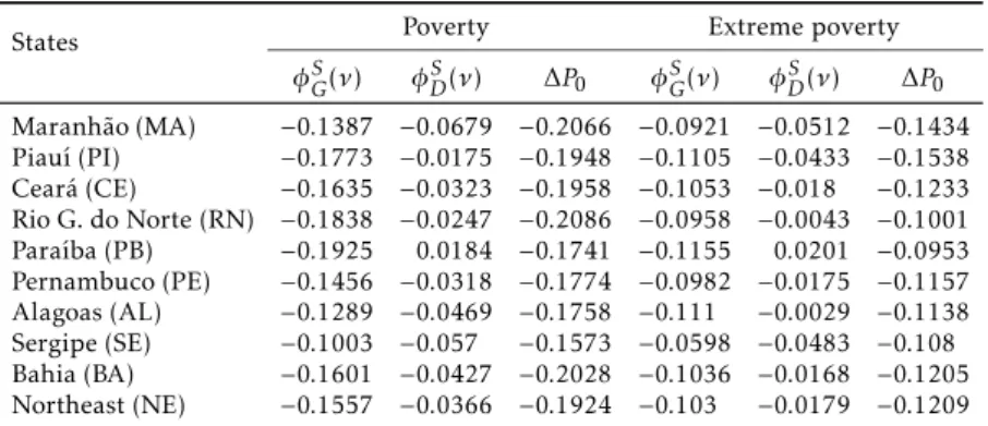
poverty and extreme poverty based on the minimum wage. Thus, half 2003 minimum wage (MW) was used to define the poverty line and a quarter of it, for extreme poverty. These lines were adjusted to reflect 2008 values. The minimum wage in 2003 was R$240,00, which generated a line of poverty and indigence of R$120,00 and R$60,00, respectively. In 2008, these values cor-responded to, respectively, R$154,30 and R$77,15. These lines were used to generate the results of Shapley methodology, which can be seen in Table 1.
In Table 1, considering the Northeast as a whole, it is possible to observe that when income distribution remains constant — that is, at 2003 level — the growth of per capita average household income would have been responsible for a reduction of approximately 15 percentage points in poor people ratio. For extreme poverty, the component “growth” would have reduced the level of poverty, given the constant inequality, in 10 pp. The factor distribution reinforced, although to a lesser extent, the growth effect. In a scenario where
Table 1: Decomposition of poverty and extreme poverty (P0) into two
components: growth (φSG) and distribution (φDS), 2003-2008
States Poverty Extreme poverty
φGS(ν) φDS(ν) ∆P0 φS
G(ν) φSD(ν) ∆P0
Maranhão (MA) −0.1387 −0.0679 −0.2066 −0.0921 −0.0512 −0.1434
Piauí (PI) −0.1773 −0.0175 −0.1948 −0.1105 −0.0433 −0.1538
Ceará (CE) −0.1635 −0.0323 −0.1958 −0.1053 −0.018 −0.1233
Rio G. do Norte (RN) −0.1838 −0.0247 −0.2086 −0.0958 −0.0043 −0.1001
Paraíba (PB) −0.1925 0.0184 −0.1741 −0.1155 0.0201 −0.0953
Pernambuco (PE) −0.1456 −0.0318 −0.1774 −0.0982 −0.0175 −0.1157
Alagoas (AL) −0.1289 −0.0469 −0.1758 −0.111 −0.0029 −0.1138
Sergipe (SE) −0.1003 −0.057 −0.1573 −0.0598 −0.0483 −0.108
Bahia (BA) −0.1601 −0.0427 −0.2028 −0.1036 −0.0168 −0.1205
Northeast (NE) −0.1557 −0.0366 −0.1924 −0.103 −0.0179 −0.1209
have reduced poverty by 3.6 pp, and extreme poverty, by 1.7 pp. Therefore, it was observed that the increase in the per capita household income explained approximately 81% of poverty reduction and 85% of extreme poverty reduc-tion in the Northeast. Marinho & Soares (2003), using methodology and pe-riod different from that used in this study (1985-1999), decomposed the
varia-tion of poverty in the components of growth and concentravaria-tion (distribuvaria-tion). According to their results, the decline in poverty in the Northeast region was explained entirely by the growth factor (−55.73%). Inequality, unlike what was observed in this study, also played an important role (44.27%), though in order to increase the proportion of poor.
The state of Rio Grande do Norte showed the best result for the drop in the number of poor people (20.86 pp). Most of this reduction was due to the growth in earnings, namely, 88% of the change in the ratio of poor people was due to the factor income. Distribution, however, contributed less signifi-cantly, having participated with only 12% of the total variation. This result is strongly associated with a small reduction in income inequality observed in the state. Between 2003 and 2008, the Gini coefficient dropped only 1.9%. In
the case of extreme poverty, the same situation was observed, i.e., the growth component explained the largest portion of the variation in poverty (96%).
Maranhão was the second state in the drop in poverty ranking (20.66 pp). The Shapley decomposition showed that income growth was primarily respon-sible for this reduction. In other words, if inequality had remained constant, poverty would have fallen — as a result of rising earnings — 13.87 pp, which is 67% of the drop in theP0index. The contribution of the redistributive factor
was lower, i.e., 33% reduction in the proportion of poor people resulted from the decreased inequality degree. With regard to extreme poverty, income dis-tribution had a slightly better performance, and was responsible for 36% of the poverty change, while the factor growth contributed with 64%.
Orair (2006) quantified the contribution of economic growth (income) and income inequality to poverty change, using a methodology different from that
applied in this article. This author used two poverty lines and several sub-periods for all states of Brazil, from 1992 to 2004. Considering Maranhão and the period between 1993 and 1995, its poverty change being similar to that observed in 2003/2008 (−0.20128), Orair (2006) found estimates similar to
Sergipe presented the second largest drop in the index of inequality, ac-cording to the Gini coefficient (6.5%). This decline led the component
distri-bution to have greater participation in the explanation of the decline of 15.73 percentage points in the proportion of poor. In other words, reduced distribu-tive inequality contributed with 36.2% of the variation of poverty. The im-portance of lessening the degree of inequality is greater for extreme poverty. Approximately 45% of the variation in extreme poverty was explained by im-proved income distribution. The contribution of the growth factor is relatively small compared to other states. One explanation for this would be the lower income growth (27%), considering, of course, the rates seen in other states of the Northeast region, with average of 43.3%.
Another point that should be mentioned is related to Paraíba. According to Table 1, poverty could have fallen even more if there had been some distri-bution of income, i.e., in a situation without change in inequality, the number of poor would fall 19.25 pp. On the other hand, if earnings remained con-stant, poverty would have increased — due to increased inequality — 1.8 pp. For indigence (extreme poverty), the result is the same, and only the growth factor is responsible for the decreased number of people below the extreme poverty line.
The results showed that the growth factor was mainly responsible for the fall in the number of poors and indigents. It is important to note that the rdpc is composed of various sources of income, namely labor income, pen-sions, rents and donations, interest income, cash transfer (Bolsa Família, for example) and other incomes sources. Among these categories, several studies have highlighted the importance of the Bolsa Família Program in combating poverty. As an example, Soares et al. (2006) emphasized that, without direct cash transfer programs, poverty and income inequality in Brazil would hardly fall to tolerable levels within a relatively short period of time.
Another issue that must be highlighted refers to labor income. This source of income is extremely important to explain the growth of earnings of the population in the Northeast region and, consequently, to poverty. For San-tos (2011), labor income was the main component of household income in the Northeast, representing 72% of the total. Moreover, in the Northeast re-gion, labor income explained 70% of the increase in household income, whose growth had been of 43.33%.
The importance of labor income in the composition of the household in-come is also observed when considering the country as a whole. For example, Soares et al. (2006) found, for the year 2004, the proportion of 72.6%, which shows the relevance of the work to the total income. Given this, the main determinants of income from work are presented below.
3.2 Decomposition based on regression
Selectivity bias is one of the problems that may occur in the process of
esti-mating earning equations.4 The Heckman procedure was used to solve this
problem. The estimates of earning equations are shown in Table 2.5
Table 2 shows that the inverse of the Mills’ ratio (lambda) is statistically significant (at 1%) in all states of the Northeast, which indicates that their inclusion was necessary to avoid selectivity bias.
In most cases, the coefficients of the equations are statistically significant
and have the expected signals, with few exceptions.
These results demonstrate that the variable years of education (Educ), who-se estimates are highly significant, has the ability to positively impact the in-come received from work. This observation is valid for all states in the North-east, which confirms the benefits of education to the income of individuals. Estimates of the variable Educ can also be interpreted as the education return rate. Thus, for each additional year of study, in the Northeast as a whole, there is an increase of 8.58% in income.6 Ceará and Bahia are the states that present
the best return rates, with values above 8.8%. With regard to Bahia, the coeffi
-cient found is very similar to that verified in Lacerda (2008), whose value was 0.0873.
Maranhão is the state where the education return rate presents the lowest level, showing that increased income, provided by each additional year of education, is lower than that observed in other states of the Northeast region. With regard to age, a proxy for experience, it is observed that the coef-ficient associated with the variable age is positive, but that related to age squared is negative. This shows that the relationship between experience and income have inverted U behavior. In other words, as the individuals gain more experience in their work environment, earnings tend to increase. However, upon reaching a certain point, income begins to decrease. Considering the Northeast as a whole, when income is maximized, the age would be around 55 years.7In Brazil, it would be, according to Kassouf (1994), 50 years for men
and approximately 46 years for women. According to the estimates of Hoff
-mann (2000), for the year 1997, the age that would maximize the Brazilians’ income would be around 50 years.
The variable gender, similarly to years of education, has a positive sign, which was expected. The results show that, for all states of the Northeast, men earn higher incomes than women. Considering the whole region, men receive on average 62.2% more than women. On the other hand, Alagoas has a much lower (though high) differential. The difference is around 33%. Ueda
& Hoffmann (2002) also found high estimates for the gender coefficient for
Brazil. The values obtained by these authors for 2002 ranged from 0.4415 to 0.4506, depending on the model. This suggests that, in Brazil, the income gap between men and women is also high.
Regarding the variable race, the signal is displayed in accordance with what was expected and, in most states, the coefficients are statistically
signifi-cant at 1% level. Then, as presented in Table 2, the income gap between white people and others (black, brown, yellow and Indian) is not as great when com-pared to the variable gender. The results suggest that income discrepancy in
5The participation equations, used in the Heckman procedure, can be seen in Table B.1 in the Appendix B.
6To avoid any inaccuracy, Wooldridge (2006) suggested using the formula 100[exp(x)−1] to calculate the percentage increase in income generated by each additional year of education, where x is the estimated coefficient of the variable education.
Sa n to s an d V ie ir a E co n om ia A p lic ad a, v.1 7 , n .4
Table 2: Equations of income for the states of the Northeast region, Brazil, 2008
Variables MA PI CE RN PB PE AL SE BA NE
Cons. (03..84322978)∗ 3.0763
∗
(0.3697) 3.1347
∗
(0.1739) 4.0239
∗
(0.6491) 3.6189
∗
(0.5644) 3.3389
∗
(0.2139) 3.8387
∗
(0.3064) 4.0931
∗
(0.5068) 3.1884
∗
(0.1471) 3.3923
∗
(0.1071)
Educ. (00..06520067)∗ 0.0713
∗
(0.0107) 0.0899
∗
(0.0036) 0.0793
∗
(0.0095) 0.0808
∗
(0.0103) 0.0811
∗
(0.0042) 0.0769
∗
(0.0064) 0.0852
∗
(0.0091) 0.0889
∗
(0.0037) 0.0823
∗
(0.0021)
Id (00..43361037)∗ 0.4722
∗∗
(0.1420) 0.5996
∗
(0.0776) (00..30072287) 0.4948
∗
(0.1861) 0.6835
∗
(0.0784) 0.4999
∗
(0.1081) 0.327
∗∗∗
(0.1872) 0.7184
∗
(0.0536) 0.5918
∗
(0.0397)
Id2 −(00..03480115)∗ −0.0402
∗
(0.0162) −0.0571
∗
(0.0091) −(00..01620264) −0.0405
∗∗∗
(0.0224) −0.0669
∗
(0.0097) −0.0383
∗
(0.0119) −(00..01750237) −0.0669
∗
(0.0064) −0.0538
∗
(0.0047)
Sexo (00..51180599)∗ 0.6261
∗
(0.0705) 0.5755
∗
(0.0493) 0.4181
∗
(0.0799) 0.3661
∗
(0.0825) 0.4226
∗
(0.0357) 0.2863
∗
(0.0608) 0.4345
∗
(0.1018) 0.4932
∗
(0.0283) 0.4839
∗
(0.0211)
Cor (00..15990352)∗ (00..0852)0852 0.1381
∗
(0.0222) 0.1175
∗
(0.0368) (00..0389)0241 0.1485
∗
(0.0249) 0.1046
∗∗∗
(0.0546) 0.0926
∗∗
(0.0389) 0.1259
∗
(0.0273) 0.1223
∗
(0.0123)
Occup1 (00..54270729)∗ 0.8395
∗
(0.0939) 0.6224
∗
(0.0635) 0.5434
∗
(0.1013) 0.5233
∗
(0.0826) 0.497
∗
(0.0536) 0.6046
∗
(0.0785) 0.5652
∗
(0.0887) 0.4754
∗
(0.0485) 0.5529
∗
(0.0259)
Occup2 (00..07730538)∗ 0.1845
∗∗∗
(0.0472) (00..09170554) (00..02230621) (00..0555)0457 −(00..03240324) (00..067)0325 (00.0782.084) −(00..03750272) 0.0315
∗∗∗
(0.0938)
Industry (00..32041053)∗ 0.6052
∗
(0.1407) 0.2211
∗
(0.0817) 0.3849
∗
(0.0664) 0.2894
∗∗∗
(0.1546) 0.2777
∗
(0.0621) 0.3262
∗
(0.1109) −(00..06991663) 0.2555
∗
(0.0595) 0.2514
∗
(0.0397)
Service (00..36650907)∗ 0.7038
∗
(0.1096) 0.3783
∗
(0.0522) 0.4587
∗
(0.0764) 0.4482
∗
(0.1151) 0.2569
∗
(0.0541) (00..1189)23 0.2122
∗∗
(0.0974) 0.2254
∗
(0.0482) 0.3373
∗
(0.0275)
Construction (00..34270729)∗ 0.6865
∗
(0.1492) 0.4937
∗
(0.0586) 0.4379
∗
(0.0856) 0.5214
∗
(0.1198) 0.2321
∗
(0.0555) 0.1556
∗
(0.1142) 0.2822
∗
(0.0667) 0.2406
∗
(0.0532) 0.3602
∗
(0.0288)
Lambda −(00..34640478)∗ −0.37874
∗
(0.1001) −0.3347
∗
(0.0525) −0.5102
∗
(0.1513) −0.4133
∗
(0.1302) −0.1606
∗
(0.0607) −(00..29810663) −0.4136
∗
(0.1343) −0.1966
∗
(0.0463) −0.2937
∗
(0.0291)
Note: Educ.= years of education, Occup1 = professionals/technicians; Occup2 = workers who have graduated from high school; Occup. (base) = Workers (blue collars).∗significant at 1%;∗∗significant at 5%;∗∗∗significant at 10%. The standard-deviations (linearized) are between brackets. The
Maranhão, in terms of race, is the highest in the region. In that state, white people receive, on average, 17.34% more than individuals in the base category. In the Northeast as a whole, this difference was 13%.
Discrimination in the labor market occurs when individuals or groups with equal average qualifications (skills) do not receive the same mean income (Lundberg & Startz 1983). Therefore, income inequalities observed between genders and between races, after assessing the other variables, suggest that there is some kind of discrimination in the labor market in the Northeast re-gion of Brazil.
The variablesOcup1, andOcup2 andOcup3 (base) were inserted into the
model to analyze the effects of allowing the analysis of the type of workers’
occupation on income. According to the results, the sign of the variable Ocup1 — which refers to managers in general, practitioners of sciences and arts and technicians — is in line with what was expected. In other words, workers in this group have incomes well above those that form the base group, the manual laborers (blue collars). For the Northeast as a whole, the group Ocup1 receives on average 73.8% more than workers of the base category.
The income of mid-level workers (Ocup2) is higher than that observed in
Ocup3, except for Pernambuco and Bahia. Piauí has the highest coefficient
related to variableOcup2, suggesting that the income of workers that occupy
intermediate positions is, on average, 20.3% higher than that found in the base category.
According to the theories of compensating wage differentials and efficiency
wages, income inequality may be partially explained by the characteristics pe-culiar to each economic activity. By virtue of being controlled, in earning equations, the effects of the variables education, age, gender, race and
profes-sional activity, the estimates of the variables Ocup1 and Ocup2 may reflect what is established by the mentioned theories, i.e., the advantages or disad-vantages existing in jobs (theory of compensating differentials) as well as the
internal policies adopted by some firms that set wages higher than in the labor market (efficiency wages theory) may be important to determine the salary of
workers.
The regressors Industry, Service, Construction and Agriculture (base) were included in the model to analyze the impacts of working in their respective sectors on income. All these variables have expected signs and were statisti-cally significant, except for the variable industry in the state of Bahia. Accord-ing to estimates, the occupations in industry, service and construction gener-ate income well above that recorded in the base cgener-ategory (agriculture). Given this and based on the dual labor market theory, which assumes the existence of two market segments, primary and secondary, we can say that agriculture in the Northeast is the industry that best fits the secondary segment, which, according to the dual labor market theory, is characterized by low wages, lack of stability and career advancement and higher manpower turnover.
(age and age squared), Gender, Race (Color) and Occupation (Ocup1 and
Ocup2). The results are presented in Table 3.
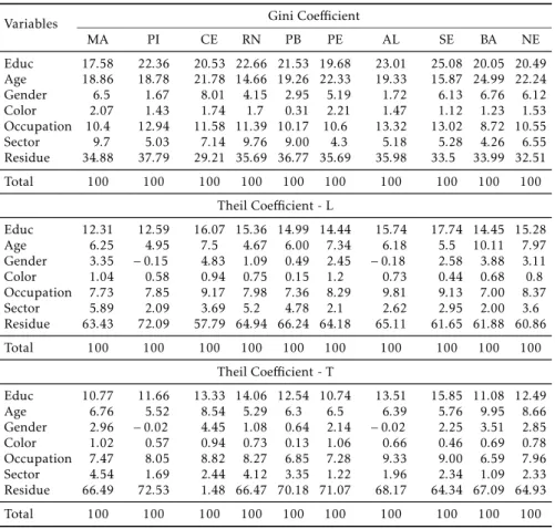
Table 3: Decomposition (Shapley) based on the earning equation estimated by the Heckman procedure (%), 2008
Variables Gini Coefficient
MA PI CE RN PB PE AL SE BA NE
Educ 17.58 22.36 20.53 22.66 21.53 19.68 23.01 25.08 20.05 20.49
Age 18.86 18.78 21.78 14.66 19.26 22.33 19.33 15.87 24.99 22.24
Gender 6.5 1.67 8.01 4.15 2.95 5.19 1.72 6.13 6.76 6.12
Color 2.07 1.43 1.74 1.7 0.31 2.21 1.47 1.12 1.23 1.53
Occupation 10.4 12.94 11.58 11.39 10.17 10.6 13.32 13.02 8.72 10.55
Sector 9.7 5.03 7.14 9.76 9.00 4.3 5.18 5.28 4.26 6.55
Residue 34.88 37.79 29.21 35.69 36.77 35.69 35.98 33.5 33.99 32.51
Total 100 100 100 100 100 100 100 100 100 100
Theil Coefficient - L
Educ 12.31 12.59 16.07 15.36 14.99 14.44 15.74 17.74 14.45 15.28
Age 6.25 4.95 7.5 4.67 6.00 7.34 6.18 5.5 10.11 7.97
Gender 3.35 −0.15 4.83 1.09 0.49 2.45 −0.18 2.58 3.88 3.11
Color 1.04 0.58 0.94 0.75 0.15 1.2 0.73 0.44 0.68 0.8
Occupation 7.73 7.85 9.17 7.98 7.36 8.29 9.81 9.13 7.00 8.37
Sector 5.89 2.09 3.69 5.2 4.78 2.1 2.62 2.95 2.00 3.6
Residue 63.43 72.09 57.79 64.94 66.24 64.18 65.11 61.65 61.88 60.86
Total 100 100 100 100 100 100 100 100 100 100
Theil Coefficient - T
Educ 10.77 11.66 13.33 14.06 12.54 10.74 13.51 15.85 11.08 12.49
Age 6.76 5.52 8.54 5.29 6.3 6.5 6.39 5.76 9.95 8.66
Gender 2.96 −0.02 4.45 1.08 0.64 2.14 −0.02 2.25 3.51 2.85
Color 1.02 0.57 0.94 0.73 0.13 1.06 0.66 0.46 0.69 0.78
Occupation 7.47 8.05 8.82 8.27 6.85 7.28 9.33 9.00 6.59 7.96
Sector 4.54 1.69 2.44 4.12 3.35 1.22 1.96 2.34 1.09 2.33
Residue 66.49 72.53 1.48 66.47 70.18 71.07 68.17 64.34 67.09 64.93
Total 100 100 100 100 100 100 100 100 100 100
According to the results, when the Gini coefficient is used, the models
ex-plain between 62.2 (Piauí) and 70.8% (Ceará) of total inequality, which shows the good explanatory power of the decomposition method. According to Wan & Zhou (2005), models that explain only 30 to 40% of inequality, leaving the rest to the residue, cannot provide reliable estimates.
The results obtained by the Gini index reveal that, in five states (Piauí, Rio Grande do Norte, Paraíba, Alagoas and Sergipe), education was primarily re-sponsible for income inequality, explaining at least 21% of it. In the Northeast region as a whole, the Gini coefficient in 2008 was approximately 0.55. Out
of this total, education contributed with 20.49%.
Maranhão was the state with the lowest value for the contribution of educa-tion to inequality. This result may be related to the rate of return to educaeduca-tion in that state. Table 2 shows that Maranhão has the lowest coefficient in the
Age is another important variable to explain inequality in the Northeast, a proxy for experience. Table 3 shows the contribution of age using the Gini index, which ranged from 14.7 (Rio Grande do Norte) to 25% (Bahia). In the Northeast region as a whole, the variable experience was mainly responsible for the high Gini index, contributing with approximately 22%.
Overall, the results related to education and age are consistent with the human capital theory, which establishes the link between income inequality and qualification of individuals. The positive relationship between education and inequality, observed in Table 3, is justified by the fact that most educated people (with more years of education) tend to earn higher incomes. Neverthe-less, depending on where one lives and on financial conditions, not everyone has the same access to education.
The variables that characterize the jobs, joined in occupation (Table 3), were included in the analysis to capture the likely effects established by the
compensating wage differentials and efficiency wages theories. According to
these theories, the earning differentials can be explained both by the
advan-tages and disadvanadvan-tages present in each job (compensating wage differentials)
and by the wages above the market price (efficiency wages theory) that firms
pay to their employees. For these theories, the differences between jobs were
extremely important in explaining income inequality in the Northeast region of Brazil. The results demonstrate that these variables accounted, on average, for 10.55% of the Gini index, i.e., the group is ranked as the third largest contributor to inequality in the region. In Alagoas, the group Occupation ex-plained 13.32% of the Gini coefficient.
The variables related to workers’ sector of activity, which were included to take into account the theory of dual labor market, had the ability to ex-plain 6.55% of the Gini index, which is a relatively significant value. To some extent, these results agree with the theory of labor market segmentation, and agriculture is the sector that best fits the profile of the secondary segment. The difference between the sectors can explain part of income inequality observed
in the Northeast.
The variables gender and race show that discrimination is a major factor in income inequality. In the Northeast, these two variables accounted for 7.65% of the distributive inequality, measured by the Gini coefficient. However,
gen-der discrimination is more pronounced, and is responsible for 6.12% of total inequality. While in Piauí the income of men was approximately 87% higher than women’s, the contribution of gender to the Gini coefficient was not high
(1.67%), compared to other states. On the other hand, Alagoas had the low-est income gap between the genders (Table 2) and this difference was not so
relevant to explain income inequality.
The decomposition was also conducted using the Theil-L and Theil-T in-dices (Table 3). As observed, the share of inequality that was not explained by the variables included in the earning equation — i.e., the residue — was much greater than that observed when the Gini coefficient was used. This difference
in the residues was also found in Wan & Zhou (2005). These authors used the Gini and Theil-L coefficients in the decomposition process. In all their
estimates, the residue generated when the Theil-L coefficient was used as the
inequality measure was much greater than that observed with the use of the Gini index.
most to explain the inequality have not changed, i.e., the variables related to human capital remain the leading cause of income inequality. Differences in
values, observed when different measures are used, can be explained,
accord-ing to Wan & Zhou (2005), by the sensitivity of each index in the different
segments of the Lorenz curve and by the use of different functions of welfare.
For example, for Hoffmann (1998), the Theil-T coefficient is more sensitive
to changes in income located at the right end of the distribution, namely, the relatively richer. On the other hand, the Theil-L index is more sensitive to changes at the left end of the distribution (the poorest). Finally, the Gini coef-ficient is more sensitive to changes in incomes located at the interval with the greatest frequency density, i.e., around mode or median of the distribution.
4
Conclusions
The results above lead to some conclusions. The first is that the per capita household income in the Northeast region of Brazil was primarily responsi-ble for the decline in the number of poor, considering the years 2003 and 2008. These results are strongly related to the significant growth in income in the period observed. Although income growth has been fundamental to reduce the number of people below the poverty line, it cannot be said that it is more important than the reduction in inequality in fighting poverty, espe-cially when it comes to the Northeast, where the gap between rich and poor is very significant. The difference for income inequality among the Northeast
and the other Brazilian regions is extremely high, suggesting that inequality has much to fall. Therefore, given the relationship between income distribu-tion and poverty reducdistribu-tion, the number of poor and indigent may be reduced even more if income distribution is intensified.
In a scenario where inequality may fall more heavily, it is very important to know the main variables that can influence it. In this context, it can also be concluded that education in the Northeast was primarily responsible for the high inequality in the region. In other words, the lack of skills and low levels of education are the main factors that led the Northeastern states to have the worst income distribution in the country. Considering the prospect that the Brazilian economy will continue to grow, investment in the expansion and improvement of education will be crucial to significantly reduce the gap between those at the bottom and those at the top of the distribution. On the contrary, we may have the same condition as the one observed in the 1960s, when economic growth was accompanied by increasing inequality. At that time, there was a great demand for skilled labor, but there was not enough supply; therefore, those who were educated (higher education level) began to earn large incomes, thus worsening income distribution.
Besides the human capital variables, those related to gender and race also contributed positively to income inequality, corroborating what the theory of discrimination in the labor market states. Thus, it can be concluded that there may be some form of discrimination in the Northeast (by employers), espe-cially against women. The difference in income between men and women is
substantial — much more pronounced than the differences in income between
(curric-ula) aimed at discussing with children the issue of prejudice, to prevent the appearance of any type of discrimination in future generations. Moreover, public policies — or laws providing for stiffer penalties — against
discrimina-tion would also be extremely important at reducing income concentradiscrimina-tion in the Northeastern states.
Bibliography
Alejos, L. (2003), Contribution of the determinants of income inequality in guatemala, Instituto de investigaciones económicas y sociales. Universidad Rafael Kandívar: Guatemala.
Aliprantis, C. D. & Chakrabarati, S. K. (2000), Games and decision making, Oxford university press.
Araar, A. & Duclos, J. Y. (2009), Dasp: Distributive analysis stata package, Pep & cirpÉe e world bank, laval university.
Baye, F. M. (2006), ‘Growth, redistribution and poverty changes in cameroon: a shapley decomposition analysis’, Journal of African Economics15(4), 543– 570.
Cirino, J. F. (2008), Participação feminina e rendimento no Mercado de tra-balho: análise de decomposição para o Brasil e as regiões metropolitanas de Belo Horizonte e Salvador. 188f. Tese (Doutorado em Economia Apli-cada), PhD thesis, Departamento de Economia Rural, Universidade Federal de Viçosa, Minas Gerais.
Fields, G. (2003), ‘Accounting for income inequality and its change: a new method, with application to the distribution of earnings in the united states’, Research in Labour Economicspp. 1–38.
Fields, G. & Yoo, G. (2000), ‘Falling labour income inequality in korea’s eco-nomic growth: patterns and underlying causes’,Review of Income and Wealth pp. 139–159.
Foster, J., Greer, J. & Thorbecke, E. (1984), ‘A class of decomposable poverty measures’,Econometrica52(3), 761–766.
Guimarães Neto, L. (2004), O nordeste, o planejamento regional e as armadil-has da macroeconomia.,in‘Desigualdades Regionais’, Superintendência de Estudos Econômicos e Sociais da Bahia, pp. 153–175.
Gunatilaka, R. & Chotikapanich, D. (2009), ‘Accounting for sri lanka’s expen-diture inequality 1980-2002: regression-based decomposition approaches’, Review of Income and Wealth55(4), 882–905.
Heckman, J. J. (1979), ‘Sample selection bias as a specification erro’, Econo-metrica47(1), 153–161.
Hoffmann, R. (1998), Distribuição de renda, medidas de desigualdade e
po-breza, Edusp, São Paulo.
Hoffmann, R. (2000),Mensuração da desigualdade e da pobreza no Brasil,
num-ber 3, IPEA, chapter Desigualdade e pobreza no Brasil.
Hoffmann, R. & Kassouf, A. L. (2005), ‘Deriving conditional and
uncondi-tional marginal effects in log earnings equations estimated by heckman’s
pro-cedure’,Applied Economics37(11), 1303–1311.
Kassouf, A. L. (1994), ‘The wage rate estimation using the heckman proce-dure’,Revista de Econometria14(1), 89–107.
Kassouf, A. L. (1997), ‘Retorno à escolaridade e ao treinamento nos setores urbanos e rural do brasil.’,Revista de Economia e Sociologia Rural35(2), 59– 76.
Lacerda, F. C. C. (2008), Desigualdade de rendimentos na bahia: estimação de equações de rendimentos com base nos microdados da pnad 2005,in‘IV Encontro de Economia Bahiana’, Salvador, BA.
Lundberg, S. J. & Startz, R. (1983), ‘Private discrimination and social
in-tervention in competitive labor market’, The American Economic Review
73(3), 340–347.
Marinho, E. & Soares, F. (2003), Impacto do crescimento econômico e da concentração de renda sobre a redução da pobreza nos estados brasileiros,in ‘XXXI Encontro Nacional de Economia’, Vol. 31, ANPEC, Porto Seguro.
Montet, C. & Sierra, D. (2003), Game theory and economics, Palgrave macmillan. 487.
Morduch, J. & Sicular, T. (2002), ‘Rethinking inequality decomposition, with evidence from rural china’,Economic Journalpp. 93–106.
Ney, M. G. (2006), Educação e desigualdade de renda no meio rural brasileiro, PhD thesis, Instituto de Economia da Unicamp, Campinas, São Paulo. 117f. Tese (Doutorado em Economia Aplicada).
Orair, R. O. (2006), Como crescimento e desigualdade afetam a pobreza?, Master’s thesis, Instituto de economia da UNICAMP, São Paulo. 125f. Disser-tação (Mestrado em Economia).
Osborne, M. J. & Rubinstein, A. (1994), A course in game theory, Cambridge, ma.
Resende, M. & Wyllie, R. (2006), ‘Retornos para educação no brasil: evidên-cias empíricas adicionais’,Economia Aplicada10(3), 349–365.
Rocha, S. (2000), Pobreza e desigualdade no brasil: o esgotamento dos efeitos distributivos do plano real, Texto para discussão, Instituto de Pesquisa Econômica Aplicada. No 721.
Salardi, P. (2002), How much of brazilian inequality can explain? an attempt of income differentials using pnad 2002. 2005, Acesso em: 06 dez. 2009.
Santos, V. F. (2011), Efeitos do crescimento e redução da desigualdade de renda na pobreza da região nordeste do Brasil - 2003-2008, PhD thesis, Uni-versidade Federal de Viçosa, Viçosa - MG. 140f. Tese (Doutorado em Econo-mia Aplicada.
Shapley, L. S. (1953), A value for n-person game, Vol. 28, Ann. Math. Stud., chapter Contributions to the theory of games II, pp. 307–317.
Shorrocks, A. F. (1999), Decomposition procedures for distributional anal-ysis: a unified framework based on the shapley value, University of essex. Mimeogr.
Soares, F. V., Soares, S., Medeiros, M. & G., O. R. (2006), Cash transfer pro-grammes in brazil: impacts on inequality and poverty. Working Paper n.21, IPC-IG.
Ueda, E. M. & Hoffmann, R. (2002), ‘Estimando o retorno da educação no
brasil.’,Revista Economia Aplicada6(2), 209–238.
Wan, G. (2004), ‘Accounting for income inequality in rural china: a regression-based approach’, Journal of Comparative Economics. 32(2), 348– 363.
Wan, G. & Zhou, Z. (2005), ‘Income inequality in rural china:
regression-based decomposition using household data’, Review of Development
Eco-nomics9(1), 107–120.
Wooldridge, J. M. (2006),Introdução à econometria: uma abordagem moderna, Thompson Learning, São Paulo.
Appendix A
Shapley value
Shapley (1953) introduced one of the most used solution concepts in cooper-ative game theory. This concept (value), according to Montet & Sierra (2003), has the ability to summarize, in a coalition game, the complex possibilities faced by economic agents (players) in a single number, called the Shapley value. Therefore, in an allocation problem, the Shapley value allows or sug-gests the division of profits or common costs arising from the grand coalition. LetN={1,2, . . . , m}be a finite set of players. Then, a nonempty subset ofNis
called a coalition.8
For each coalitionS⊆N , ν(S) is a value, either positive or negative, which is available for division among members of the coalitionS.9This is carried out based on the average marginal contribution of each player to the coalition.
According to Osborne & Rubinstein (1994), the marginal contribution from playerito any coalitionS, withi<Sin a given game, can be measured as
fol-lows:
8The method developed by Shapley can be applied to various allocation problems, such
as water resource management, allocation of taxes, landing fees at airports, etc. (Aliprantis & Chakrabarati 2000).
9In other words,νis a characteristic function that associates to each subset S a real number
∆
i(S) =ν(S∪ {i})−ν(S) (12) Thus, the Shapley value of the player i, denoted byφSi(ν) is given by:
φSi (ν) = 1 |N|!
X
R∈ℜ
∆i(Si(R)),for eachi∈N (13)
whereℜ denote the set of all orders ofN andSi(R) denote the set of the players precedingiin the orderR. By conversion, 0! = 1 andν(∅) = 0.
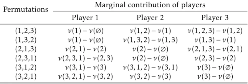
Intuitively, the Shapley method can be understood by considering, for sim-plicity, three players: 1, 2 and 3. Therefore, we haveN={1,2,3}. Thus, the
number of permutations that can be made from the setNis 6, that is,N! = 6.
These permutations or orderings can be observed in the first column of Table A.1.
Table A.1: Shapley value in a game with three players
Permutations Marginal contribution of players
Player 1 Player 2 Player 3
(1,2,3) ν(1)−ν(∅) ν(1,2)−ν(1) ν(1,2,3)−ν(1,2)
(1,3,2) ν(1)−ν(∅) ν(1,3,2)−ν(1,3) ν(1,3)−ν(1)
(2,1,3) ν(2,1)−ν(2) ν(2)−ν(∅) ν(2,1,3)−ν(2,1)
(2,3,1) ν(2,3,1)−ν(2,3) ν(2)−ν(∅) ν(2,3)−ν(2)
(3,1,2) ν(3,1)−ν(3) ν(3,1,2)−ν(3,1) ν(3)−ν(∅)
(3,2,1) ν(3,2,1)−ν(3,2) ν(3,2)−ν(3) ν(3)−ν(∅)
To calculate the marginal contribution of each player in any coalition, it is necessary to define the set of players preceding playeri. Taking column 2 of
Table A.1 (player 1) as an example, it is observed that, in the first ordering, the set of players preceding player 1 is∅(empty set). Therefore, the empty set is
one of the possible coalitions. The other sets, referring to other orderings, are {2},{2,3},{3}and{3,2}. The logic is the same for the other players.
After defining the set of players that precede player i, it is possible to measure the marginal contributions of player i when he joins the coalition
S. Thus, according to the equation 12, the marginal contribution of player 1, taking into account the first ordering, is equal toν(1)−ν(∅), whereν(1) and ν(∅) are, respectively, the values associated with the coalition 1 (∅∪ {1}) and
the coalition∅.
From equation 14, and knowing thatN! = 6, it is possible to measure the
Shapley value for each player. Considering the player 1, one has
φ1=16
X
R∈ℜ
∆i(Si(R)), (14)
whereP(.) is the sum of column 2 of Table A.1.
E ff ec ts of gr ow th an d re d u ct io n of in co m e in eq u al ity 66 5
Variables MA PI CE RN PB PE AL SE BA NE
Cons. −(04..42691839)∗ −4.1358
∗
(0.1925) −3.5940
∗
(0.0332) −3.9817
∗
(0.1730) −4.1205
∗
(0.0802) −4.1933
∗
(0.1016) −4.1580
∗
(0.1984) −3.9905
∗
(0.2276) −3.9024
∗
(0.0874) −3.9719
∗
(0.0467)
Educ. (00..07340066)∗ 0.0462
∗
(0.0067) 0.0637
∗
(0.0034) 0.0659
∗
(0.0060) 0.0819
∗
(0.0062) 0.0769
∗
(0.0040) 0.0612
∗
(0.0049) 0.0561
∗
(0.0076) 0.0693
∗
(0.0032) 0.0689
∗
(0.0016)
Sexo (00..9780595)∗ 0.9284
∗
(0.0563) 0.7417
∗
(0.0332) 0.8943
∗
(0.0559) 0.9254
∗
(0.0615) 0.9118
∗
(0.0339) 0.8397
∗
(0.0602) 0.7362
∗
(0.0697) 0.8801
∗
(0.0246) 0.8737
∗
(0.0151)
Cor −(00..0600533) −(00..6165)0654 −0.0528
∗∗∗
(0.0305) −0(0..04380444) (00..03090375) −0(0..02150312) 0.1308
∗
(0.0409) (00..05680493) −0.0765
∗∗
(0.0308) −0.0476
∗
(0.0133)
Id (02..01231105)∗ 2.0556
∗
(0.0876) 1.6515
∗
(0.0506) 1.8421
∗
(0.1063) 1.7657
∗
(0.0483) 1.8639
∗
(0.0489) 1.8286
∗
(0.1167) 1.9355
∗
(0.1151) 1.8117
∗
(0.0497) 1.8083
∗
(0.0254)
Id2 −(00..24210141)∗ −0.2396
∗
(0.0098) −0.1945
∗
(0.0674) −0.0220
∗
(0.0141) −0.2158
∗
(0.0076) −0.2275
∗
(0.0063) −0.2252
∗
(0.0162) −0.2400
∗
(0.0175) −0.2173
∗
(0.0067) −0.2170
∗
(0.0034)
Children (00..11580438)∗∗ (00..04680645) −(00..0314)0089 −(00..07640639) (00..06880436) 0.0518
∗∗∗
(0.0278) −(00..01310469) −(00..05430627) (00..00390281) 0.0245
∗∗∗
(0.0131)
head of house (00..56330730)∗ 0.5161
∗
(0.0811) 0.6020
∗
(0.0278) 0.4287
∗
(0.0936) 0.6252
∗
(0.0541) 0.4818
∗
(0.0336) 0.7162
∗
(0.0664) 0.5877
∗
(0.0608) 0.4867
∗
(0.0343) 0.5391
∗
(0.0171)
Number of observation 4,814 3,881 18,095 4,809 5,534 18,157 3,884 4,521 24,635 88,330
Considered population 4,228,031 2,130,021 6,028,229 2,267,435 2,759,061 6,064,189 2,177,670 1,487,961 9,885,248 37,027,845
F statistic (prob.) 31.00∗ 100.58∗ 216.19∗ 43.67∗ 25.44∗ 144.10∗ 38.57∗ 53.73∗ 159.32∗ 448.70∗
Note: Educ.= years of education.∗significant at 1%;∗∗significant at 5%.∗∗∗significant at 10%. The (linear) standard-deviations are in