Closed and Open Loop Subspace System Identification of the Kalman Filter

(1)

Closed and Open Loop Subspace System

Identification of the Kalman Filter

David Di Ruscio

Telemark University College, P.O. Box 203, N-3901 Porsgrunn, Norway

Abstract

Some methods for consistent closed loop subspace system identification presented in the literature are analyzed and compared to a recently published subspace algorithm for both open as well as for closed loop data, the DSR e algorithm. Some new variants of this algorithm are presented and discussed. Simulation experiments are included in order to illustrate if the algorithms are variance efficient or not.

Keywords: Subspace, Identification, Closed loop, Linear Systems, Modeling

1 Introduction

A landmark for the development of so called subspace system identification algorithms can be said to be the algorithm for obtaining a minimal state space model re-alization from a series of known Markov parameters or impulse responses, i.e., as presented byHo and Kalman

(1966). Subspace system identification have been an important research field during the last 2.5 decades.

Larimore(1983,1990) presented the Canonical Variate

Analysis (CVA) algorithm. The N4SID algorithm pre-sented byOverschee and de Moor (1994) and further-more, subspace identification of deterministic systems, stochastic systems as well as combined deterministic linear dynamic systems are developed and discussed in detail in Overschee and de Moor(1996) and where also the Robust N4SID was presented. In the standard N4SID an oblique projection is used and this method was biased for colored inputs and an extra orthogo-nal projection, in order to remove the effect of future inputs on future outputs, was included in the Robust N4SID. See also Katayama (2005) and the references therein for further contributions to the field. These subspace system identification algorithms may in some circumstances lead to biased estimates in case of closed loop input and output data.

A subspace system identification method, based on

observed input and output data, which estimates the system order as well as the entire matrices in the Kalman filter including the Kalman filter gain matrix,

K, and the square root of the innovations covariance matrix, F, was presented in Di Ruscio (1994, 1996). This algorithm is implemented in the DSR function in the D-SR Toolbox for MATLAB. The DSR estimate of the innovation square root covariance matrix F is consistent both for open loop as well as for closed loop data. The DSR method was compared with other al-gorithms and found to give the best model in compar-ison to the other methods, based on validation, and on a real world waste and water example in Sotomayor et al.(2003a,b).

The DSR e method presented in Di Ruscio (2008) and used in the thesis by Nilsen (2005) is a simple subspace system identification method for closed and open loop systems. DSR e is a two stage method where the innovations process is identified consistently in the first step. The second step is simply a deterministic system identification problem.

InQin and Ljung(2003),Weilu et al.(2004) a

(2)

in traditional subspace algorithms in case of feedback in the data. An extended version is presented in Qin

et al.(2005).

The main contributions of this paper can be itemized as follows:

• An extended presentation, further discussions and details of the DSR e algorithm inDi Ruscio(2008) are given in this paper. In particular the second stage of the algorithm, the deterministic identi-fication problem, is discussed in detail and some solution variants are discussed and presented in Sections6.1,6.2and6.3 of this paper.

• The PARSIM algorithm by Qin et al. (2005) is considered, and in particular the PARSIM-E al-gorithm inQin and Ljung(2003) is discussed and presented in detail in Section5.1. In the PARSIM-E algorithm some Markov parameters are re-estimated. A modified version of the PARSIM-E algorithm which does not re-estimate the Markov parameters is presented in Section5.2. The mod-ified version follows the lines in the PARSIM-S algorithm (Algorithm 2) inQin et al.(2005). The PARSIM-S method is biased for direct closed loop data, as pointed out inQin et al.(2005), while the modified algorithm in Section5.2is consistent for closed loop subspace identification.

• Due to the lack of software implementation of the PARSIM E algorithm from the authors this al-gorithm is discussed and implemented along the lines in Section5.1and the “past-future” data ma-trix Eq. presented in Di Ruscio (1997) and im-plemented as a MATLAB m-file function. The Matlab m-file code of the PARSIM-E algorithm is enclosed in the Appendix.

This implementation of the PARSIM E algorithm is compared with the DSR e function in the D-SR Toolbox for MATLAB, and a new variant of the

dsr emethod is discussed. This new variant con-sists of an Ordinary Least Squares (OLS) step for solving a deterministic identification problem for computing the entire Kalman filter model matri-ces.

• The DSR e algorithm is a subspace system identi-fication algorithm which may be used to estimate the entire Kalman filter model matrices, includ-ing the covariance matrix of the innovations pro-cess and the system order, directly from known in-put and outin-put data from linear MIMO systems. Simulation experiments on a linear MIMO closed loop system is given in this paper, and the algo-rithm is shown to give promising estimation results

which are comparable to the corresponding esti-mates from the Prediction Error Method (PEM). • Monte Carlo simulation experiments, on two ex-amples (a SISO and a MIMO system), are pre-sented which show that the DSR e algorithm out-performs the PARSIM-E method for closed loop subspace system identification. Interestingly, the DSR e algorithm is on these two examples shown to give as efficient parameter estimates as the Pre-diction Error Method (PEM).

The contributions in this paper are believed to be of interest for the search for an optimal subspace identifi-cation algorithm for open and closed loop systems. The PARSIM-E and DSR methods may be viewed as sub-space methods which are based on matrix Eqs. where the states are eliminated from the problem.

Noticing that if the states of a linear dynamic system are known then the problem of finding the model matri-ces is a linear regression problem, see e.g., Overschee

and de Moor (1996). Some methods for closed loop

subspace identification with state estimation along the lines of the higher order ARX model approach pre-sented in Ljung and McKelvey (1995) are presented

in Jansson (2003, 2005) and Chiuso (2007). In this

class of algorithms the states are estimated in a prelim-inary step and then the model matrices are estimated as a linear regression problem. InLjung and McKelvey

(1995) a method denoted, SSNEW, with MATLAB m-file code is presented. InJansson(2003) a method de-noted SSARX was presented, and inJansson(2005) a three step method denoted, NEW, is presented. Chiuso

(2007) presents the methods denoted, PBSID and PB-SID opt, and shows some asymptotic similarities with the SSARX and the PBSID algorithms. It is also shown that the PBSID opt algorithm is a row weighted ver-sion of the SSNEW algorithm inLjung and McKelvey

(1995). Furthermore, Chiuso (2007) stated that the PBSID opt algorithm is found to be asymptotically variance efficient on many examples but not in gen-eral.

It would be of interest to compare these methods with the DSR e algorithm, in particular for systems with a low signal to noise ratio. The SSNEW m-file in the original paper by Ljung and McKelvey (1995) would be a natural starting point in this work, but this is outside the scope of this paper and is a topic for further research, where the results are believed to be of interests.

(3)

discussed in connection with the “past-future” data matrix presented in Di Ruscio (1997). In Section 5 the PARSIM-E method,Weilu et al.(2004),Qin et al.

(2005), for closed loop system identification is discussed as well as a variant of this method. In Section 6 we discuss thedsr emethod with a new variant of imple-mentation in case of a known system order. In Section 7 some examples which illustrate the behavior of the algorithms are presented. Finally some concluding re-marks follow in Section8.

2 Problem formulation

We will restrict ourselves to linearized or linear state space dynamic models of the form

xk+1 = Axk+Buk+Cek, (1)

yk = Dxk+Euk+F ek, (2)

withx0as the initial predicted state and where a series of N input and output data vectors uk andyk ∀ k=

0,1, . . . , N−1 are known, and where there is possible feedback in the input data. In case of output feedback the feed through matrix is zero, i.e. E = 0. Also for open loop systems the feed through matrix may be zero. We will include a structure parameter g = 0 in case of feedback data or for open loop systems in which

E = 0, andg= 1 for open loop systems when E is to be estimated. Furthermore, for the innovations model (1) and (2)ekis white with unit covariance matrix, i.e.

E(ekeTk) =I .

Note that corresponding to the model (1) and (2) on innovations form we may, if the system is not pure deterministic, define the more common Kalman filter on innovations form by defining the innovations asεk=

F ek and then K = CF−1 is the Kalman filter gain.

Hence, the Kalman filter on innovations form is defined as

xk+1 = Axk+Buk+Kεk, (3)

yk = Dxk+Euk+εk, (4)

where the innovations process εk have covariance

ma-trix E(εkεTk) =F FT.

The quintuple system matrices (A, B, C, D, E, F) and the Kalman filter gain K are of appropriate di-mensions. The problem addressed in this paper is to determine these matrices from the known data. Both closed and open loop systems are addressed.

3 Notations and definitions

Hankel matrices are frequently used in realization the-ory and subspace system identification. The special

structure of a Hankel matrix as well as some matching notations, which are frequently used throughout the paper, are defined in the following.

Definition 3.1 (Hankel matrix) Given a vector se-quence

sk ∈ Rnr ∀ k= 0,1,2, . . . , (5)

wherenr is the number of rows insk.

Define integer numbers j, i and nc and define the matrixSj|i ∈Rinr×nc as follows

Sj|i

def

= 

   

sj sj+1 sj+2 · · · sj+nc−1

sj+1 sj+2 sj+3 · · · sj+nc

..

. ... ... . .. ...

sj+i−1 sj+i sj+i+1 · · · sj+i+nc−2 

   

,

which is defined as a Hankel matrix because of the spe-cial structure. A Hankel matrix is symmetric and the elements are constant across the anti-diagonals. The integer numbers j, i and nc have the following inter-pretations:

• jstart index or initial time in the sequence used to formSj|i, i.e.,sj, is the upper left vector element

in the Hankel matrix.

• iis the number of nr-block rows inSj|i.

• ncis the number of columns in the Hankel matrix

Sj|i.

One should note that this definition of a Hankel ma-trix Sj|i is slightly different to the notation used in

Overschee and de Moor(1996) (pp. 34-35) where the

subscripts denote the first and last element of the first column in the block Hankel matrix, i.e. using the nota-tion inOverschee and de Moor(1996) a Hankel matrix

U0|i is defined by puttingu0 in the upper left corner and ui in the lower left corner and hence U0|i would

havei+ 1 rows.

Examples of such vector processes,sk, to be used in

the above Hankel-matrix definition, are the measured process outputs,yk ∈Rm, and possibly known inputs,

uk ∈Rr.

Definition 3.2 (Basic matrix definitions)

The extended observability matrix, Oi, for the pair

(D, A) is defined as

Oi

def =



   

D DA

.. .

DAi−1 

   

∈ Rim×n, (6)

(4)

The reversed extended controllability matrix, Cd i,

for the pair (A, B) is defined as

Cd i

def

= Ai−1_B _Ai−2_B _{· · ·} _B _∈ _Rn×ir_, ₍₇₎

where the subscript i denotes the number of block columns. A reversed extended controllability matrix,

Cs

i, for the pair (A, C) is defined similar to (7), i.e.,

Cs i

def

= Ai−1_C _Ai−2_C _{· · ·} _C _∈ _Rn×im_, ₍₈₎

i.e., withB substituted with C in (7). Thelower block triangular Toeplitz matrix, Hd

i ∈ R

im×(i+g−1)r _{, for}

the quadruple matrices (D, A, B, E).

Hd i

def =



     

E 0m×r 0m×r · · · 0m×r

DB E 0m×r · · · 0m×r

DAB DB E · · · 0m×r

..

. ... ... . .. ...

DAi−2_B _DAi−3_B _DAi−4_B _{· · ·} _E 

     

where the subscripti denotes the number of block rows andi+g−1is the number of block columns, and where

0m×r denotes the m×r matrix with zeroes. A lower

block triangular ToeplitzmatrixHs i ∈R

im×im _{for the}

quadruple (D, A, C, F) is defined as

Hs i

def =



     

F 0m×m 0m×m · · · 0m×m

DC F 0m×m · · · 0m×m

DAC DC F · · · 0m×m

..

. ... ... . .. ...

DAi−2_C _DAi−3_C _DAi−4_C _{· · ·} _F 

     

Given two matrices A ∈ Ri×k _and _B _∈ _Rj×k_{, the}

orthogonal projection of the row space of A onto the row space ofB is defined as

A/B=ABT₍_BBT₎†_B. ₍₉₎ The following property is used

A/

A B

=A. (10)

Proof of Eq. (10) can be found in e.g.,Di Ruscio(1997).

4 Background theory

Consider the “past-future” data matrix, Eq. (4) in the paper Di Ruscio (1997). This same equation is also presented in Eq. (27) in the Di Ruscio (1997) paper. We have

YJ|L =

Hd

L OLC˜Jd OLC˜Js





UJ|L+g−1

U0|J

Y0|J





+ OL(A−KD)JX0|1+HLsEJ|L, (11)

where ˜Cs

J =CJs(A−KD, K) is the reversed extended

controllability matrix of the pair (A−KD, K), and ˜

Cd J =C

d

J(A−KD, B−KE) is the reversed extended

controllability matrix of the pair (A−KD, B−KE), and whereCd

J andC s

J are defined in Eqs. (7) and (8),

respectively.

One should here note that the term OL(A −

KD)J_X

0|1 → 0 exponentially as J approaches infin-ity. Also note Eq. (43) inDi Ruscio(2003) with proof, i.e.,

XJ|1= _˜

Cd J C˜Js

U0|J

Y0|J

+ (A−KD)J_X

0|1, (12) which relates the ”past” data matrices, U0|J

and Y0|J to the ”future” states XJ|1 =

xJ xJ+1 · · · xN−(J+L) .

Note that Eq. (11) is obtained by putting (12) into the following common matrix equation in the theory of subspace system identification, i.e.

YJ|L=OLXJ|1+HLdUJ|L+g−1+HLsEJ|L. (13)

Eq. (11) is of fundamental importance in connection with subspace system identification algorithms. One problem in case of closed loop subspace identification is that the future inputs,UJ|L+g−1in the regressor ma-trix are correlated with the future innovations,EJ|L.

Proof 4.1 (Proof of Eq. (11))

From the innovations model, Eqs. (1) and (2), we find Eq. (13), where definitions for the Hankel matrices

YJ|L,UJ|L+g−1 and EJ|L as well as the matrices OL,

Hd

L andHLs are given in Section3.

From the Kalman filter on innovations form, Eqs. (3) and (4), we obtain the optimal Kalman filter pre-diction, y¯k, of the output, yk, as y¯k = Dxk +Euk,

and the Kalman filter state Eq.,xk+1=Axk+Buk+

K(yk−y¯k). From this we find Eq. (12) for the states.

Finally, puttingXJ|1given by Eq. (12) into Eq. (13)

proves Eq. (11).

The matrices Hd L and H

s

L with Markov parameters

are block lower triangular Toeplitz matrices. This lower triangular structure may be utilized in order to overcome the correlation problem, and recursively com-puting the innovations sequences,εJ|1,. . .,εJ|L in the

innovations matrix EJ|L. This was the method for

closed loop subspace identification proposed by Qin

et al.(2005) andWeilu et al.(2004). This method

de-noted PARSIM is discussed in the next Section5 and compared to the DSR e method,Di Ruscio (2008), in an example in Section7.1.

(5)

identification is built as a two stage method where the innovations sequences,εJ|1, are identified from Eq.

(11) in the first step. Noticing that puttingL= 1 and

g= 0 (no direct feed through term in the output equa-tion) then we see that Eq. (11) also holds for closed loop systems, i.e., we have

YJ|1=

DC˜d J DC˜

s J

U0|J

Y0|J

+F EJ|1. (14) Hence, the DSR F matrix estimates in Di Ruscio

(1996) is consistent also for closed loop data. The sec-ond step is an optimal OLS step and hence solved as a deterministic problem. The DSR e method is further discussed in Section6.

5 Recursive computation of

innovations

5.1 The PARSIM-E Algorithm

We will in this section work through the PARSIM-E method presented by Qin and Ljung (2003), and further discussed in Weilu et al. (2004) and in the same instant indicate a drawback with this method (i.e. Markov parameters are recomputed and large matrices pseudo inverted when J large) and show how we may overcome this. This was also noticed inQin and Ljung

(2003). In order to give a simple view and understand-ing of the PARSIM method we present a few of the first iterations in the algorithm.

Step 1:

i

= 0

LetL= 1, J→ ∞andg= 0 in (11) and we have

YJ|1=

DC˜d J DC˜Js

U0|J

Y0|J

+εJ|1. (15) From Eq. (15) we find estimate of the innovations

εJ|1 = F EJ|1 as well as the indicated matrix in the regression problem, i.e., DC˜d

J DC˜ s J

. Hence, an ordinary Least Squares (OLS) problem is solved. This step is identical to the first step in the DSR e method.

Step 2:

i

= 1

We may now express from Eq. (11)

YJ+1|1=

DB DAC˜d

J DAC˜ s J DK



  

UJ|1

U0|J

Y0|J

εJ|1 

  

+F EJ+1|1. (16)

From Eq. (16) we find estimate of the innovations

εJ+1|1 = F EJ+1|1. The regression problem increases

in size and the matrix DB DAC˜d

J DAC˜ s J DK

is estimated as an OLS problem.

Hence, at this stage the non-zero part of the first block rows in the Toeplitz matrices Hd

L and HLs, i.e.

the Markov parametersDB andDK, respectively, are computed. Proceeding in this way each non-zero block row, Hd

i|1 and His|1, in the Toeplitz matrices is com-puted as follows.

Step 3:

i

= 2

YJ+2|1=

h

Hd

2|1 DA2C˜Jd DA2C˜Js H2|1s i



      

UJ|1

UJ+1|1

U0|J

Y0|J

εJ|1

εJ+1|1 

      

+F EJ+2|1, (17)

where

H2|1d =

DAB DB ∈ Rm×2r, (18)

and

Hs

2|1=

DAK DK ∈ Rm×2m. (19)

εJ+2|1=F EJ+2|1as well as an estimate of the matrix

DAB DB DA2_C_˜d

J DA2C˜ s

J DAC DC

. Hence, at this stage the Markov parameters DB

(6)

Step 4:

i

:= 3

YJ+3|1=

h

Hd

3|1 DA2C˜

d

J DA3C˜ s J H

s

3|1 i



          

UJ|1

UJ+1|1

UJ+2|1

U0|J

Y0|J

εJ|1

εJ+1|1

εJ+2|1 

          

+F EJ+3|1, (20)

where

Hd

3|1=

DA2_B _DAB _DB _∈ _Rm×3r_, ₍₂₁₎

and

H3|1s =

DA2_K _DAK _DK _∈

Rm×3m. (22) From Eq. (20) we find estimate of the innovations

εJ+3|1=F EJ+3|1as well as the indicated matrix with model parameters.

Step 5: General case

i

= 2

_,

3 _{, . . . , L}

_.

YJ+i|1=

h

Hd i|1 DA

i_C_˜d J DA

i_C_˜s J H

s i|1

i 

    

UJ|i

U0|J

Y0|J

εJ|i−1

εJ+i−1|1 

    

+F EJ+i|1 (23)

where

Hd i|1=

DAi−1_B _{· · ·} _DB _∈ _Rm×ir_, ₍₂₄₎

and

His|1=

DAi−1_K _{· · ·} _DK _∈

Rm×im. (25) From Eq. (23) we find estimate of the innovations

εJ+i|1 =F EJ+i|1. The process given by Eq. (23) is

performed fori= 0,1,2, . . . , L in order to find the ex-tended observability matrix OL+1 and to use the shift invariance technique in order to findA.

This means that at each new iteration (repetition)

i one new last row εJ+i−1|1 is included in the regres-sion matrix on the right hand side of Eq. (23) and one new innovations sequence εJ+i|1 =F EJ+i|1 is identi-fied. This procedure is performed for i = 0,1, . . . L

in order to identify OL+1 and using the shift invari-ance method for calculatingOL andOLA. HereLis a

user specified horizon into the future for predicting the number of states. Note also that the regression matrix to be inverted at each step increases in size for each new iteration.

We can see that at each iteration, i.e. in particu-lar fori≥2 unnecessary Markov parameters are esti-mated. However, it is possible to exploit this by sub-tracting known terms from the left hand side of Eq. (23). Note that at iterationi= 1 the Markov param-eters DB and DK are computed and these may be used in the next stepi= 2. This modified strategy is discussed in the next Section5.2.

Software implementation of the PARSIM-E algo-rithm has not been available so an own Matlab m-file function has been implemented. This function is avail-able upon request.

5.2 A modified recursive algorithm

We will in this section present a modified version of the PARSIM-E method presented by Qin and Ljung

(2003), and utilize the block lower triangular structure of the Toeplitz matricesHd

L andH s

L. In the

PARSIM-E algorithm some of the Markov parameters are re-computed in the iterations for i = 2,3, . . . , L even if they are known from the previous iterations. The al-gorithm will in this section be modified.

A modified version of PARSIM was also commented upon in Qin et al. (2005), i.e., in Algorithm 2 of the paper a sequential PARSIM (PARSIM-S) algorithm is presented. This algorithm utilizes the fact that some Markov parameters in the term Hd

i|1UJ|i are known

at each iteration i ≥ 2. However, the term Hs i|1εJ|i

is omitted and the innovations, εJ|1, . . ., εJ+L|1 are not computed in this algorithm, and the PARSIM-S method is biased for direct closed loop data, also com-mented upon in Remark 2 of that paper. To make the PARSIM-S applicable to closed loop data, they refer to the innovation estimation approach as proposed in

Qin and Ljung(2003).

The iterations for i = 0 and i = 1 are the same as in the previous PARSIM-E method in Eqs. (15) and (16). Hence, at this stage the Markov parameters

(7)

Step 3:

i

= 2

YJ+2|1−DBUJ+1|1−DKεJ+1|1=

DAB DA3_C_˜d

J DA3C˜Js DAK



  

UJ|1

U0|J

Y0|J

εJ|1 

  

+F EJ+2|1. (26)

εJ+2|1 =F EJ+2|1 and new Markov parameters in the indicated matrix on the right hand side are computed.

Step 4:

i

:= 3

DA2_B _DA2_C_˜d

J DA2C˜ s

J DA2K



  

UJ|1

U0|J

Y0|J

εJ|1 

  

+F EJ+3|1. (27)

εJ+3|1=F EJ+3|1as well as the indicated matrix with model parameters. As we see the matrix of regression variables on the right hand side is unchanged during the iterations and one matrix inverse (projection) may be computed once.

Step 5: General case

i

= 2

_,

3 _{, . . . , L}

_.

YJ+i|1−

Hid−1|1

z }| {

DAi−2_B _{· · ·} _DB _U

J+1|i−1

−

Hs i−1|1

z }| {

DAi−2_K _{· · ·} _DK _ε

J+1|i−1=

DAi−1_B _DAi_C_˜d J DA

i_C_˜s J DA

i−1_K 

  

UJ|1

U0|J

Y0|J

εJ|1 

  

+F EJ+i|1, where fori≥2

Hd i|1 =

DAi−1_B _{· · ·} _DB

= h DAi−1_B _Hd i−1|1

i

, (28) and

Hs i|1 =

DAi−1_K _{· · ·} _DK

= h DAi−1_K _Hs i−1|1

i

. (29) From this general case we find estimate of the in-novations εJ+i|1 = F EJ+i|1. The process given are

performed for i = 2, . . . , L in order to find the ex-tended observability matrixOL+1 and to use the shift invariance technique in order to find A. Furthermore the Markov parameters in matricesHd

L|1andH

s L|1 are identified. See next section for further details.

5.3 Computing the model parameters

In both the above algorithms the model matrices (A, B, K, D) may be determined as follows. The fol-lowing matrices are computed, i.e.,

ZJ|L+1 =

OL+1C˜Jd OL+1C˜Js

= OL+1 _˜

Cd J C˜

s J

, (30)

and the matrices with Markov parameters

HLd|1=

DAL_B _DAL−1_B _{· · ·} _DB _, ₍₃₁₎

Hs L|1=

DAL_C _DAL−1_K _{· · ·} _DK _. ₍₃₂₎ From this we find the system order, n, as the num-ber of non-zero singular values of ZJ|L+1, i.e. from

a Singular Value decomposition (SVD) of theZJ|L+1 matrix. From this SVD we also find the extended observability matricesOL+1 and OL. Furthermore A

may be found from the shift invariance principle, i.e.

A=OL†OL+1(m+1 : (L+1)m,:) andD=OL(1 :m,:).

The B and K matrices may simply be computed by forming the matrices OLB andOLK from the

es-timated matrices Hd

L+1|1 and H

s

L+1|1 and then pre-multiplyOLBandOLKwith the pseudo inverseO_L† =

(OT

LOL)−1OTL.

5.4 Discussion

The two methods investigated in this section do not seem to give very promising results compared to the

dsr e method. It seems that the variance of the pa-rameter estimates in general is much larger than the

dsr eestimates.

The reason for the high variance in the PARSIM-E method is probably that the algorithm is sensitive to data with low signal to noise ratios, and the reason for this is that “large” matrices are pseudo inverted when J is “large”. Recall that in Eq. (11) the therm

(8)

the states X0|J are correlated with the data matrix

with regression variables. In practice the past horizon parameter J is finite and the term is negligible. How-ever, a matrix of larger size than it could have been is inverted and this gives rise to an increased variance, compared to the DSR e method in the next Section6. It is also important to recognize that only the first in-novations sequence, εJ|1, really is needed, as pointed

out in Di Ruscio (2008) and that it seems unneces-sary to compute the innovation sequences, εJ+i|1, ∀

i = 1, . . . L, and then forming the innovations matrix

EJ|L+1, i.e.,

EJ|L+1= 

        

εJ|1

εJ+1|1 .. .

εJ+i|1 .. .

εJ+L|1 

        

. (33)

Only the first row, εJ|1, is actually needed in order

to find the model matrices as we will show in the next Section6. Since unnecessary future innovations rows in

EJ|L+1 matrix are computed, this probably also gives rise to large variances in estimates from the PARSIM algorithm.

In the PARSIM strategy, Section 5, a matrix with increasing size,ir+Jr+Jm+mi= (J+i)r+(J+i)m= (J+i)(m+r), is pseudo inverted at each new iteration

i= 0,1,2, . . . , L. The matrix to be inverted increases in size during the iterative process when 0 ≤ i ≤ L. Both the pseudo inverse problem and the iterations give rise to this large variance. Updating techniques for this matrix inverse may be exploited, however.

The modified PARSIM method in Section 5.2 was also implemented with a QR factorization and the re-cursive algorithm implemented in terms of the R fac-tors only. This strategy seems not to improve the vari-ance considerably and the varivari-ances are approximately the same. The reason is probably that J should be “large” for the method to work. It is interesting to note that in this modified algorithm only a matrix of row sizer+rJ+mJ+m= (J+ 1)(r+m) is pseudo in-verted and that this regressor matrix is held unchanged during the iterations and is inverted once.

We believe that thedsr emethod, with a consistent estimate of the innovations process in a first step, fol-lowed with an optimal estimation of a noise free deter-ministic subspace identification problem, or if the order is known solved by an optimal OLS (ARX) step leads us to the lower bound on the variance of the param-eter estimates. Note that the first step in the dsr e

method is a consistent filtering of the output signal,

yJ|1, into a signal part, y_Jd_|1, and a noise innovations

part, εJ|1. We will in the next Section 6 discuss the

dsr emethod.

6 The DSR e algorithm

In Di Ruscio (2008) a very simple, efficient subspace

system identification algorithm which works for both open as well as for closed loop data was presented. This algorithm was developed earlier and presented in an internal report in (2004) and used inNilsen(2005). In this section an improved and extended presentation of the algorithm is presented.

In the DSR e algorithm the signal content, yd J|1, of the future data, yJ|1 =

yJ yJ+1 . . . yN−1 ∈

Rm×(N−J), is estimated by projecting the “past” onto the “future”, and in case of closed loop data when the direct feed-through term is zero (E= 0), i.e. estimated by the following projection

yd

J|1=DXJ|1=YJ|1/

U0|J

Y0|J

, (34)

where the projection operator “/” is defined in Eq. (9), and where we have used that for largeJ or asJ → ∞ we have that

XJ|1/

U0|J

Y0|J

=XJ|1, (35)

which may be proved from Eq. (12) by using Eq. (10). The past data matrices,U0|J andY0|J, are

uncorre-lated with the future innovations sequence, EJ|1. In the same stage the innovations sequenceεJ|1=F EJ|1 in Eq. (15) is then consistently estimated as

εJ|1=F EJ|1=YJ|1−YJ|1/

U0|J

Y0|J

. (36) Note that both the signal part,yd

J|1, and the innovation part,εJ|1, are used in the dsr ealgorithm.

For open loop systems we may have a direct feed through term in the output equation, i.e., E 6= 0 and with an output Eq. yk=Dxk+Euk+F ek we obtain

YJ|1=DXJ|1+EUJ|1+F EJ|1, (37) and the signal parts may in this case be computed as,

yd

J|1=DXJ|1+EUJ|1=YJ|1/ 



UJ|1

U0|J

Y0|J



, (38)

where we have used Eq. (10). Furthermore, the inno-vations are determined by

εJ|1=F EJ|1=YJ|1−YJ|1/ 



UJ|1

U0|J

Y0|J



(9)

The algorithm is a two step algorithm where in the first step the output data are split into a signal part,

yd

J|1, and a noise (innovations) part,εJ|1=F EJ|1, i.e.,

as

yJ|1=ydJ|1+εJ|1. (40) This step of splitting the future outputs, yJ|1, into a

signal part, DXJ|1, and an innovations part, εJ|1, is

of particular importance in the algorithm. We propose the following choices for solving this first step in the algorithm:

• Using a QR (LQ) decomposition. Interestingly, the square root of the innovations covariance ma-trix,F, is also obtained in this first QR step, as in

Di Ruscio(1996). Using the definitions or the QR

decomposition gives approximately the same re-sults in our simulation examples. One should here note that when the QR decomposition is used also theQfactors as well as theRfactors are used. We have the from the QR decomposition

U0|J+g

Y0|J+1

=

R11 0

R21 R22

Q1

Q2

, (41) where g = 0 for closed loop systems and systems with no direct feed through term in the output Eq., i.e., whenE= 0. For open loop systems and when we want to estimate the direct feed through matrixE we putg= 1. From, the decomposition (41) we have

yd

J|1=R21Q1, (42)

εJ|1=R22Q2, (43) and we notice that also the Q sub matrices are used. Notice also that we may take F = R22 or compute a new QR decomposition ofεJ|1in order to estimateF.

• Another interesting solution to this step is to use a truncated Conjugate Gradient (CG) algorithm,

Hestenes and Stiefel (1952), in order to compute

the projection. The CG algorithm is shown to be equivalent with the Partial Least Squares al-gorithm inDi Ruscio(2000) for univariate (single output) systems. This will include a small bias but the variance may be small. This choice may be considered for noisy systems in which PEM and the DSR e method have unsatisfactory variances or for problems where one has to chose a “large” past horizon parameterJ. However, one have to consider a multivariate version, e.g. as the one proposed inDi Ruscio(2000).

This step of splitting the future outputs, yJ|1, into

a signal part,DXJ|1, and an innovations part,εJ|1, is

consistent and believed to be close to optimal whenJ

is “large”.

The second step in the dsr e algorithm is a deter-ministic subspace system identification step if the sys-tem order has to be found, or an optimal deterministic Ordinary Least Squares (OLS) step if the system order is known, for finding the Kalman filter model. Using PEM for solving the second deterministic identification problem may also be an option.

Hence, the future innovations εJ|1 = F EJ|1 (noise part) as well as the given input and output data are given and we simply have to solve a deterministic iden-tification problem. Note also that if the system order,

n, is known this also is equivalent to a deterministic OLS or ARX problem for finding the model. This method is effectively implemented through the use of QR (LQ) factorization, see the D-SR Toolbox for Mat-lab functiondsr e.m(unknown order) anddsr e ols

or PEM if the order is known.

At this stage the innovations sequence,εJ|1, and the

noise free part,yd

J|1, of the outputyJ|1are known from the first step in the DSR e algorithm. Hence we have to solve the following deterministic identification problem

xk+1 = Axk+

B K

uk

εk

, (44)

yd

k = Dxk, (45)

where not only the input and output data,uk, and,ykd,

respectively, are known, but also the innovations, εk,

are known. Hence, the data

uk

εk

yd k

 



∀ k=J, J+ 1, . . . , N−1 (46)

are known, and the model matrices (A, B, K, D) may be computed in an optimal OLS problem.

The second step in the DSR e method is best dis-cussed as a deterministic identification problem where we will define new input and output data satisfying a deterministic system defined as follows

yk:=ydk

uk:=

uk

εk

 



∀ k= 1,2, . . . , N (47)

where N := N −J is the number of samples in the time series to be used in the deterministic identification problem. Hence we have here defined new outputs,yk,

from all corresponding samples in the noise free part

yd

J|1 ∈ Rm×K where the number of columns is K =

N−J. Similarly, new input datauk∈Rr+m, is defined

from the sequence uJ|1 =

(10)

of the original input data, and from the the computed innovations inεJ|1=

εJ εJ+1 · · · εN−1 . In the examples of Section 7 we illustrate the sta-tistical properties of the method on closed loop data, and we show that DSR e is as optimal as PEM, and far more efficient than the PARSIM method.

We believe that the first step in the DSR e algorithm is close to optimal. Since we have some possibilities for implementing the second step in the algorithm, i.e., the deterministic identification problem, at least in the multiple output case. We discuss some possibilities for the second step separately in the following subsections. This second deterministic identification step is believed to be of interest in itself.

6.1 Deterministic subspace identification

problem

Step 2 in the dsr e.m implementation in the D-SR Toolbox for MATLAB is basically as presented in this subsection.

Consider an integer parameter Lsuch that the sys-tem order, n, is bounded by 1 ≤ n ≤ mL. As an example for a system with m = 2 outputs andn = 3 states it is sufficient withL= 2.

From the known deterministic input and output data

uk

yk

∀ k= 0,1, . . . , N define the data matrix equa-tion

Y1|L= ˜ALY0|L+ ˜BLU0|L+g, (48)

where the matrices are given by ˜

AL = OLA(OLTOL)−1OLT, (49)

˜

BL =

OLB HLd

−A˜L

Hd

L 0mL×r

.

(50) The same data as used in Eq. (48), i.e. Y0|L+1 =

Y0|L

YL|1

andU0|L+g are used to form the matrix Eq.

Y0|L+1=OL+1X0|J+HLd+1U0|L+g. (51)

There are some possibilities to proceed but we suggest estimating the extended observability matrix from Eq. (51) and theB,Ematrices as an optimal OLS problem from Eq. (48), using the correspondingRsub matrices from the following LQ (transpose of QR) factorisation, i.e.,

U0|L+g

Y0|L+1

=

R11 0

R21 R22

Q1

Q2

. (52) Due to the orthogonal properties of the QR factorisa-tion we have

R22=OL+1X0|JQT2, (53)

and the system order, n, the extended observability matrix OL+1, and thereafter A and D, may be

esti-mated from an SVD ofR22, and using the shift invari-ance technique. An alternative to this is to form the matrix Eq.

¯

R22= ˜ALR22, (54) and estimate the system order as the n largest non-zero singular values of the mL singular values of the matrixR22. Here ¯R22 is obtained asR22with the first

m block row deleted and R22 as R22 with the last m block row deleted. Using only the n largest singular values we have from the SVD that R₂₂=U1S1V1T and we may choseOL=U1 and findAfrom Eq. (54), i.e., as

A=UT

1R¯22V1S1−1. (55) Note that there are common block rows in R22 and

¯

R22. This may be utilized and we may use

A=UT

1 _¯

U1

R22(Lm+ 1 : (L+ 1)m,:)V1S1−1

, (56) which is used in the DSR algorithms. This means that we, for the sake of effectiveness, only use the truncated SVD of R22 and the last block row inR22 in order to compute an estimate of theA matrix. The D matrix is taken as the firstmblock row inOL=U1. This way

of computing theAandD matrices is a result fromDi

Ruscio(1994).

Finally, the parameters in theBandEmatrices are estimated as an optimal OLS step, using the structure of matrix ˜BL and the equation

¯

R21= ˜ALR21+ ˜BLR11, (57) where ¯R21 is obtained as R21 with the first m block row deleted and R21 as R21 with the last m block row deleted. Since ˜AL now is known the problem

˜

BLR11= ¯R21−A˜LR21 may be solved for the parame-ters inB (andE for open loop systems) as an optimal OLS problem in the unknown (n+m)rparameters inB

andE,Di Ruscio(2003). We also mention in this

con-nection that it is possible to include constraints in this OLS step, in order to e.g. solve structural problems, e.g. withK= 0 as in output error models.

6.2 Deterministic OLS/ARX step 2

(11)

Specify a prediction horizon parameter,L, as speci-fied above. We have the input and output ARX model

yk=A1yk−L+· · ·+ALyk−1

+B1uk−L+· · ·+BLuk−1, (58) where Ai ∈ Rm×m and Bi ∈ Rm×r ∀i= 1, . . . , L are

matrices with system parameters to be estimated. We only consider the case with a delay of one sample, i.e. without direct feed through term (E= 0) in Eq. (2).

From the observed data form the OLS/ARX regres-sion problem

YL|1=θ

Y0|L

U0|L

(59)

where the parameter matrix,θ,∈Rm×L(m+r)_{, is given} by

θ= A1· · ·ALB1· · ·BL

. (60)

This regression problem is effectively solved through a LQ (transpose of QR problem) factorization.

Note that for single output systems then we simply may choseL =n and the state space model matrices

A,B,K andD are determined simply from the corre-spondence withθand the observer canonical form.

For multiple output systems we may choseLsmaller than the system order according to the inequality 1≤

n≤ mL. Hence, a non-minimal state space model of ordermLon block observer form is constructed directly from the OLS estimate,θ, i.e.,

A= 

       

AL Im 0 · · · 0

..

. ... . .. 0

Ai 0 . .. 0

..

. ... Im

A1 0 . . . 0 

       

, B= 

      

BL

.. .

Bi

.. .

B1 

      

,

D= Im 0 · · · 0

. (61)

Hence, the A matrix in the non-minimal state space model has the Ai ∈ Rm×m matrices in the left block

column. TheB matrix in the non-minimal state space model of order n≤mL is constructed from theBi ∈

Rm×r_{matrices. Noticing that the model has the same}

impulse response matrices as the underlying system, a state space realization with ordern is constructed by Hankel matrix realization theory through a Singular Value Decomposition (SVD).

Using the realization algorithm in Ho and Kalman

(1966), Hankel matrices H1|L = OLCJ and H2|L =

OLACJ are constructed from impulse response

matri-ces hi = CAi−1B ∀ i = 1, . . . , L+J, where L+J

is the number of impulse response matrices. Using

the SVD realization algorithm inZeiger and McEwen

(1974) gives the model matricesA, B and D and the system order,n.

The above method with outline of implementation is included in the D-SR Toolbox for MATLAB function

dsr e ols.m.

6.3 Discussion

We have tried with different implementations of the deterministic identification problem in the second step of the DSR e algorithms. In Section6.1we presented a deterministic subspace identification problem for iden-tifying both the system order,n, as well as the model matrices A, B, K, D, E. Interestingly, this choice was found to be the best one for all simulation experiments. To our knowledge this subspace system identification method is both consistent and close to efficient for closed as well as for open loop data. The efficiency of the algorithm is illustrated by simulation experiments in the section of examples.

In Section 6.2 we implemented the deterministic identification problem as an OLS/ARX step. However, due to the identification of the block observer form non minimal state space model of order mL and the need for model reduction, this did not match the low vari-ance estimates from thedsr e algorithm with the de-terministic subspace solution as presented in Section 6.1.

An optimal PEM step for direct identification of the parameters of an n-th order canonical form state space model of the deterministic identification second step in the DSR e algorithm is also considered. This option does not in general improve the estimates and in some examples gave larger variance than the dsr e imple-mentation. However, this option should be investigated further.

Finally one should note that there are two horizon integer parameters involved in the DSR e algorithm. The first parameterJ defines “past” input and output data which is used to remove noise from the “future” outputs. The parameter J should be chosen “large” such that the error termD(A−KF)J_X

0|J in the first

projection is negligible. Note that the size of this term may be analyzed after one run of the algorithm. How-ever, on our simulation experiments J in the range 6 ≤ J ≤ 10 gave parameter estimates with similar variances as the PEM estimates, see the examples in Section7. The horizonJ is only used in the first step so that the second step of the algorithm is independent of this parameter.

In the second step a prediction horizon parameterL

(12)

and in the multiple output caseLshould be chosen as small as possible, as a rule of thumb. Note however that we have observed that it often is better to chose

L = 2 than L = 1 even for a first order system in which n= 1. The horizon parameters may also with advantage be chosen based on model validation.

7 Numerical examples

7.1 SISO one state closed loop system

We have found that the PARSIM-E method works well on the system in Weilu et al. (2004), Case 2 below. However, we will here study a slightly modified system in which the PARSIM-E method fails to give compa-rable results as the PEM and DSR e methods, Case 1 below. Hence, this example is a counter example which shows that a method based on recursive innovations computations may give poor estimates.

Consider the following system with proper order of appearance

yk = xk+ek, (62)

uk = −Kpyk+rk, (63)

xk+1 = Axk+Buk+Kek, (64)

We consider the following two cases:

Case 1A= 0.9,B= 0.5,K= 0.6 and an initial value

x1 = 0. ek is white noise with standard deviation

0.1. For the controller we use Kp = 0.6 and rk

as a white noise signal with E(r2

k) = 1 generated

in Matlab as R = randn(N,1) and rk = R(k).

Simulation horizonN = 1000.

Case 2 Example in Weilu et al. (2004). The same parameters as in Case 1 above but with B = 1,

K= 0.5,ekis white noise with standard deviation

1 and rk as a white noise signal with E(rk2) = 2.

Simulation horizonN = 4000.

The system was simulated with discrete time in-stants 1 ≤ k ≤ N. This was done M = 100 times with different noise realizations on the innovations ek

but with the same reference signal, rk, i.e. a Monte

Carlo simulation is performed for both the above cases. For the DSR e, DSR e ols and the PARSIM-E meth-ods we used the same algorithm horizon parameters,

J = 6 and L = 3. The system identification Tool-box Ident functionpemwas used with the callsdat=

iddata(Y, U,1) andm=pem(dat, n) with system order

n= 1.

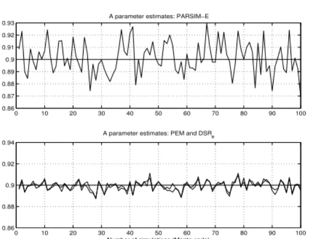
This example shows clearly that the variance of the PARSIM-E method is larger than the corresponding estimates from the DSR e algorithm which are compa-rable and as efficient as the optimal PEM estimates, in

0 10 20 30 40 50 60 70 80 90 100

0.86 0.87 0.88 0.89 0.9 0.91 0.92 0.93

A parameter estimates: PARSIM−E

0 10 20 30 40 50 60 70 80 90 100

0.86 0.88 0.9 0.92 0.94

A parameter estimates: PEM and DSR_e

Number of simulations (Monte carlo)

Figure 1:Pole estimates of the closed loop system in Example7.1 with parameters as in Case 1.

0 10 20 30 40 50 60 70 80 90 100

0.47 0.48 0.49 0.5 0.51 0.52

B parameter estimates: PARSIM−E

0 10 20 30 40 50 60 70 80 90 100

0.46 0.47 0.48 0.49 0.5 0.51 0.52

B parameter estimates: PEM and DSR_e

Figure 2:Bparameter estimates of the closed loop sys-tem in Example 7.1 with parameters as in Case 1. In Figs. 1 and 2 the PARSIM-E algorithm fails to give acceptable estimates compared to the corresponding DSR e and PEM estimates.

0 10 20 30 40 50 60 70 80 90 100

0.5 0.55 0.6 0.65 0.7

K parameter estimates: PARSIM−E

0 10 20 30 40 50 60 70 80 90 100

0.5 0.55 0.6 0.65 0.7

K parameter estimates: PEM and DSR_e

(13)

particular for the Aand B estimates as illustrated in Figures1and2. The variance of theK estimates from PARSIM are comparable with the DSR e and PEM es-timates, see Figure3. To our belief we have coded the PARSIM-E method in an efficient manner. An m-file implementation of the basic PARSIM-E algorithm is enclosed this paper. We also see that the DSR e mates are as optimal as the corresponding PEM esti-mates. We have here used the standarddsr e method as presented in Sections6 and6.1, as well as a version of DSR e with an OLS/ARX second step as presented in Section6.2, denoted DSR e ols.

For this example the PEM, DSR e and DSR e ols algorithms give approximately the same parameter es-timates. Results from DSR e and PEM are illustrated in the lower part of Figures1,2 and3.

In order to better compare the results we measure the size of the covariance matrix of the error between the estimates and the true parameters, i.e.,

P_{alg =} N M −1

M

X

i=1

(ˆθi−θ0)(ˆθi−θ0)T, (65)

as

V_{alg = trace(}P_alg), (66) where subscript “alg” means the different algorithms, i.e. PEM, DSR e, DSR e ols and PARSIM-E. Here the true parameter vector isθ0 = 0.9 0.5 0.6

T

and the corresponding estimates ˆθi =

_ˆ

A Bˆ Kˆ T_i for each estimatei= 1, . . . , M in the Monte carlo simula-tion. From the simulation results of Case 1 we obtain the results

V_{DSR e} = 0.8712, (67)

V_PEM = 0.9926, (68)

V_{DSR e ols} = 1.0565, (69)

V_PARSIM-E = 1.0774. (70) It is interesting to note that the DSR e algorithm for this example gives a lower value than PEM for the

V_{alg measure of the parameter error covariance matrix}

in Eq. (65). The reason for this is believed to be due to some default settings of the accuracy in PEM and this is not considered further.

Finally we illustrate the estimatedAparameters for the same system as in Weilu et al. (2004), i.e., with parameters in Case 2 above, see Figure 4. For this example the PARSIM-E method gives parameter esti-mates with approximately the same variance as DSR e and PEM. However, this is generally not the case as we have demonstrated in Figures1, 2and3.

0 10 20 30 40 50 60 70 80 90 100 0.85

0.9 0.95

A parameter estimates: PARSIM−E

0 10 20 30 40 50 60 70 80 90 100 0.85

0.9 0.95

A parameter estimates: PEM and DSR

e

Figure 4:Pole estimates of the closed loop system in Example 7.1 with parameters as in Case 2, and using PARSIM e, PEM and DSR e with,

B = 1.0, K = 0.5 and E(e2

k) = 1 and rk

white noise with variance E(r2

k) = 2. See

Figure1for a counter example.

0 20 40 60 80 100 14

15 16 17 18 19

hd 11

0 20 40 60 80 100 13

14 15 16 17 18

hd 12

0 20 40 60 80 100 2

2.5 3 3.5

1 ≤ i ≤ 100 hd

21

0 20 40 60 80 100 −3

−2.8 −2.6 −2.4 −2.2 −2

1 ≤ i ≤ 100 hd

22

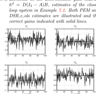
Figure 5:Elements in the deterministic gain matrix,

hd ₌ _D₍_I

3−A)B, estimates of the closed

loop system in Example7.2. Both PEM and DSR e ols estimates are illustrated and the correct gains indicated with solid lines.

0 20 40 60 80 100 2

2.5 3 3.5 4 4.5 5

hs 11

0 20 40 60 80 100 5

6 7 8 9 10

hs 12

0 20 40 60 80 100 −1.1

−1 −0.9 −0.8 −0.7 −0.6

1 ≤ i ≤ 100 hs

21

0 20 40 60 80 100 0.2

0.4 0.6 0.8 1 1.2

1 ≤ i ≤ 100 hs

22

Figure 6:Elements in the Kalman filter stochastic gain matrix,hs₌_D₍_I

3−A)−1K+I2, estimates of

(14)

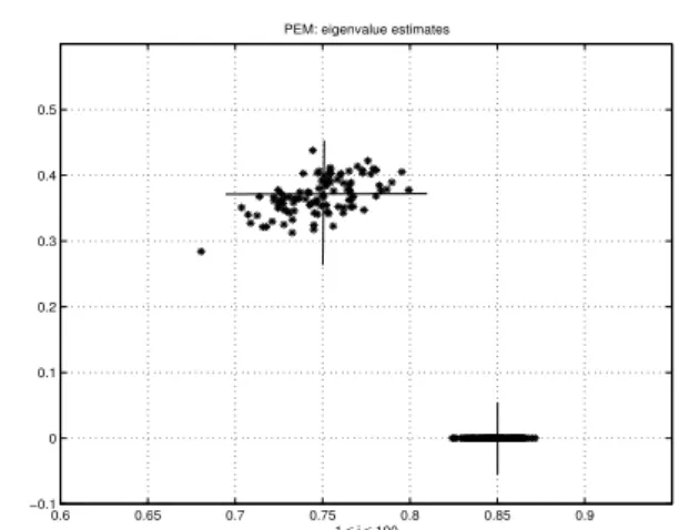
0.6 0.65 0.7 0.75 0.8 0.85 0.9 −0.1

0 0.1 0.2 0.3 0.4 0.5

1 ≤ i ≤ 100 DSR_e: eigenvalue estimates

Figure 7:Eigenvalue estimates for from the DSR e method. The correct eigenvalues are λ1 = 0.85 and a complex conjugate pair, λ2,3 = 0.75±j0.3708. Complex eigenvalues are in complex conjugate pairs. Hence, the negative imaginary part is not presented.

7.2 Closed loop MIMO

2 _×

2 _{system with}

n

= 3

_states

Consider the MIMO output feedback system

yk = Dxk+wk, (71)

uk = G(rk−yk), (72)

xk+1 = Axk+Buk+vk. (73)

where

A= 



1.5 1 0.1 −0.7 0 0.1 0 0 0.85



, B= 

 0 0 0 1 1 0



, (74)

D=

3 0 −0.6 0 1 1

. (75)

The feedback is obtained with

G=

0.2 0 0 0.2

. (76)

and rk with a binary sequence as a reference for each

of the two outputs in yk. The process noise vk and

measurements noise,wk are white with covariance

ma-trices E(vkvkT) = 0.052I3 and E(wkwTk) = 0.12I2,

re-spectively. For comparison purpose we present the de-terministic gain fromuk to yk, i.e.,

hd₌_D₍_I

3−A)−1B=

16 15

2.6667 −2.5

, (77) and the stochastic gain of the Kalman filter from inno-vations,ek to outputyk as

hs₌_D₍_I

3−A)−1K+I2=

2.8368 7.4925 −0.8998 −0.2143

(78)

0.6 0.65 0.7 0.75 0.8 0.85 0.9 −0.1

0 0.1 0.2 0.3 0.4 0.5

1 ≤ i ≤ 100 PEM: eigenvalue estimates

Figure 8:Eigenvalue estimates from PEM. The correct eigenvalues areλ1= 0.85and a complex

con-jugate pair,λ2,3= 0.75±j0.3708. Complex

eigenvalues are in complex conjugate pairs. Hence, the negative imaginary part is not presented.

A Monte Carlo simulation with M = 100 different experiments, 1 ≤ i ≤ M, is performed. The simula-tion results for the deterministic gain matrix is illus-trated in Figure5 and for the stochastic gain matrix,

hs_{, is illustrated in Figure} _{6. Furthermore we have}

presented eigenvalue estimates for both DSR e and the PEM method in Figures7and8, respectively. For the DSR e method we used the algorithm horizon param-eters,J = 6 andL= 3. The PARSIM-E estimates are out of range and are not presented.

8 Conclusion

We have in this paper investigated the subspace based method for closed loop identification proposed by

Weilu et al.(2004). Alternative versions of this method

are discussed and implemented in parallel and com-pared with the subspace identification method DSR e which works for both open and closed loop system. We have found by simulation experiments that the variance of the PARSIM-E method is much larger and in general not comparable with the DSR e and PEM algorithms. The first step in the PARSIM-E and the DSR e al-gorithms is identical. However, the methods differ in the second step. In the PARSIM-E algorithm itera-tions are included in order to estimate the future in-novations over the “future” horizon 0 ≤ i ≤ L. In the DSR e second step a simple deterministic subspace system identification problem is solved.

(15)

PARSIM-E estimates. In the PARSIM-PARSIM-E algorithm a matrix,

P = OL+1[ ˜CJdC˜Js] ∈ R(L+1)m×J(r+m), is computed

in order to compute the extended observability ma-trix OL+1. The matrix P will be of much larger size

than necessary sinceJ is “large” in order for the term

OL+1(A−KD)JX0|J to be negligible. In the DSR e

algorithm the horizon J is skipped from the second step of the algorithm and the extended observabil-ity matrix OL+1 is identified from a matrix of size (L+ 1)m×(L+ 1)(m+r) and whereLmay be chosen according to 1≤n≤mL.

We have tested the DSR e algorithm against some implementation variants using Monte Carlo simula-tions. The DSR e algorithm implemented in the D-SR Toolbox for MATLAB is found to be close to optimal by simulation experiments.

References

Chiuso, A. The role of vector autoregressive modeling in predictor-based subspace identifica-tion. Automatica, 2007. 43(6):1034–1048.

doi:10.1016/j.automatica.2006.12.009.

Di Ruscio, D. Methods for the identification of state space models from input and output measurements. In10th IFAC Symp. on System Identif.1994 . Di Ruscio, D. Combined Deterministic and

Stochas-tic System Identification and Realization: DSR-a subspace approach based on observations. Model-ing, Identification and Control, 1996. 17(3):193–230.

doi:10.4173/mic.1996.3.3.

Di Ruscio, D. On subspace identification of the ex-tended observability matrix. In36th Conf. on Deci-sion and Control. 1997 .

Di Ruscio, D. A weighted view of the partial least squares algorithm.Automatica, 2000. 36(6):831–850.

doi:10.1016/S0005-1098(99)00210-1.

Di Ruscio, D. Subspace System Identification of the Kalman Filter.Modeling, Identification and Control, 2003. 24(3):125–157. doi:10.4173/mic.2003.3.1. Di Ruscio, D. Subspace system identification of the

Kalman filter: open and closed loop systems. In

Proc. Intl. Multi-Conf. on Engineering and Techno-logical Innovation. 2008 .

Hestenes, M. R. and Stiefel, E. Methods for Conju-gate gradients for Solving Linear Systems. J. Res. National Bureau of Standards, 1952. 49(6):409–436. Ho, B. L. and Kalman, R. E. Effective construction of linear state-variable models from input/output func-tions. Regelungstechnik, 1966. 14(12):545–592.

Jansson, M. Subspace identification and arx modeling. In13th IFAC Symp. on System Identif.2003 . Jansson, M. A new subspace identification method for

open and closed loop data. InIFAC World Congress. 2005 .

Katayama, T. Subspace Methods for System Identifi-cation. Springer, 2005.

Larimore, W. E. System identification, reduced order filtering and modeling via canonical variate analysis. InProc. Am. Control Conf.1983 pages 445–451. Larimore, W. E. Canonical variate analysis in

identifi-cation, filtering and adaptive control. InProc. 29th Conf. on Decision and Control. 1990 pages 596–604. Ljung, L. and McKelvey, T. Subspace identification from closed loop data. 1995. Technical Report LiTH-ISY-R-1752, Link¨oping University, Sweden.

Nilsen, G. W. Topics in open and closed loop sub-space system identification: finite data based meth-ods. Ph.D. thesis, NTNU-HiT, 2005. ISBN 82-471-7357-3.

Overschee, P. V. and de Moor, B. N4SID: Subspace Algorithms for the Identification of Combined De-terministic Stochastic Systems. Automatica, 1994. 30(1):75–93. doi:10.1016/0005-1098(94)90230-5. Overschee, P. V. and de Moor, B. Subspace

identifica-tion for linear systems. Kluwer Acad. Publ., 1996. Qin, S. J. and Ljung, L. Closed-loop subspace

iden-tification with innovation estimation. InProc. 13th IFAC SYSID Symposium. 2003 pages 887–892. Qin, S. J., Weilu, L., and Ljung, L. A novel

sub-space identification approach with enforced causal models. Automatica, 2005. 41(12):2043–2053.

doi:10.1016/j.automatica.2005.06.010.

Sotomayor, O. A. Z., Park, S. W., and Garcia, C. Model reduction and identification of wastewater treatment plants - a subspace approach. 2003a. Latin American Applied Research, Bahia Blanca, v.33, p. 135-140, Mais Informacoes.

Sotomayor, O. A. Z., Park, S. W., and Garcia, C. Multivariable identification of an activated sludge process with subspace-based algorithms. Con-trol Engineering Practice, 2003b. 11(8):961–969.

doi:10.1016/S0967-0661(02)00210-1.

(16)

Zeiger, H. and McEwen, A. Approximate linear re-alizations of given dimensions via Ho’s algorithm.

IEEE Trans. on Automatic Control, 1974. 19(2):153.

doi:10.1109/TAC.1974.1100525.

9 Appendix: Software

function [a,d,b,k,HLd,HLs]=parsim_e(Y,U,L,g,J,n) % [A,C,B,K]=parsim_e(Y,U,L,g,J,n)

%Purpose

% Implementation of the PARSIM-E algorithm % On input

% Y,U -The output and input data matrices % L - Prediction horizon for the states % g - g=0 for closed loop systems

% J - Past horizon so that (A-KD)^J small % n - System order

if nargin == 5; n = 1; end

if nargin == 4; n = 1; J = L; end

if nargin == 3; n = 1; J = L; g = 0; end if nargin == 2; n = 1; J = 1; g = 0; L=1; end

[Ny,ny] = size(Y);

if isempty(U)==1; U=zeros(Ny,1); end

[Nu,nu] = size(U);

N = min(Ny,Nu);

K = N - L - J;

% 1. %%%%%%%%%%%%%%%%%%%%%%%%%%%%%%%%%%%%%%%%% if nargin < 6

disp(’Ordering the given input output data’) end

YL = zeros((L+J+1)*ny,K); UL = zeros((L+J+g)*nu,K); for i=1:L+J+1

YL(1+(i-1)*ny:i*ny,:) = Y(i:K+i-1,:)’; end

for i=1:L+J+g

UL(1+(i-1)*nu:i*nu,:) = U(i:K+i-1,:)’; end

%

Yf=YL(J*ny+1:(J+L+1)*ny,:); Uf=UL(J*nu+1:(J+L+g)*nu,:);

%

Up=UL(1:J*nu,:); Yp=YL(1:J*ny,:); Wp=[Up;Yp];

% general case, PARSIM-E algorithm Uf_J=[]; Ef_J=[]; OCds=[];

for i=1:L+1

Wf=[Uf_J;Wp;Ef_J];

y_Ji=YL((J+i-1)*ny+1:(J+i)*ny,:);

Hi=y_Ji*Wf’*pinv(Wf*Wf’); Zd=Hi*Wf;

e_Ji=y_Ji-Zd;

Ef_J=[Ef_J;e_Ji];

OCds=[OCds; ...

Hi(:,(i-1)*nu+1:(i-1)*nu+J*nu+J*ny)];

if i < L+1

Uf_J=UL(J*nu+1:(J+i)*nu,:); end

end

% Compute A and D/C [U,S,V]=svd(OCds);

U1=U(:,1:n); S1=S(1:n,1:n); OL=U1(1:L*ny,:);

OLA=U1(ny+1:(L+1)*ny,:); a=pinv(OL)*OLA;

d=U1(1:ny,:);

% Markov parameters HLd=Hi(:,1:L*nu);

HLs=Hi(:,L*nu+J*nu+J*ny+1:end);

% Form OL*B matrix from impulse responses in Hi ni=(L-1)*nu;

for i=1:L %ni+1,2*ni

OLB((i-1)*ny+1:i*ny,1:nu)=Hi(:,ni+1:ni+nu); ni=ni-nu;

end

b=pinv(U1(1:L*ny,:))*OLB;

% Form OL*C matrix from impulse responses in Hi Hs=Hi(:,L*nu+J*nu+J*ny+1:end);

ni=(L-1)*ny; for i=1:L

OLC((i-1)*ny+1:i*ny,1:ny)=Hs(:,ni+1:ni+ny); ni=ni-ny;

end