Instituto de F´ısica
Teoria de cordas, invariˆ
ancia conforme e
simetria BRST
H´ector Arturo Ben´ıtez del ´Aguila
Orientador: Prof. Dr. Victor de Oliveira Rivelles
Disserta¸c˜ao de mestrado apre-sentada ao Instituto de F´ısica para a obten¸c˜ao do t´ıtulo de Mestre em Ciˆencias.
Banca Examinadora:
Prof. Dr. Victor de Oliveira Rivelles (IFUSP) Prof. Dr. Diego Trancanelli (IFUSP)
Prof. Dr. Andrei Mikhailov (IFT)
Instituto de F´ısica
String Theory, Conformal Invariance and
BRST Symmetry
H´ector Arturo Ben´ıtez del ´Aguila
Orientador: Prof. Dr. Victor de Oliveira Rivelles
Disserta¸c˜ao de mestrado apre-sentada ao Instituto de F´ısica para a obten¸c˜ao do t´ıtulo de Mestre em Ciˆencias.
Banca Examinadora:
Prof. Dr. Victor de Oliveira Rivelles (IFUSP) Prof. Dr. Diego Trancanelli (IFUSP)
Prof. Dr. Andrei Mikhailov (IFT)
O principal objetivo deste trabalho ´e estudar a quantiza¸c˜ao covariante da corda bosˆonica e da supercorda RNS, explorando as simetrias envolvidas, ou seja, as simetrias BRST e conforme no caso da corda bosˆonica e as generaliza¸c˜oes correspondentes para a corda fermiˆonica. Em particular, discutimos alguns aspectos perturbativos da teoria bosˆonica e a constru¸c˜ao de operadores de v´ertice da corda fermiˆonica.
The main goal of this work is to study the covariant quantization of the bosonic and RNS string theories by exploiting the involved symmetries, namely, the BRST and conformal invariance for the bosonic string and the corresponding supersymmetric generalizations for the fermionic case. In particular, we discuss some perturbative aspects of the bosonic theory and the construction of vertex operators for the fermionic string.
Resumo iii
Abstract iv
1 Introduction 1
2 Quantization of the bosonic string 7
2.1 Basics of two dimensional conformal field theory . . . 7
2.1.1 Two dimensional conformal transformation . . . 7
2.1.2 Conformal fields in two dimensions . . . 9
2.1.3 Energy-momentum tensor . . . 11
2.1.4 Radial quantization . . . 13
2.1.5 Central charge and Virasoro algebra . . . 15
2.1.6 Highest weight states and descendant fields . . . 17
2.1.7 Matter system . . . 18
2.1.8 Ghost system . . . 21
2.2 Path integral quantization . . . 24
2.2.1 Classical local symmetries of the Polyakov’s action . . . 25
2.2.2 The S-matrix . . . 25
2.2.3 The measure for moduli . . . 30
2.2.4 U(1) current . . . 32
2.2.5 Weyl anomaly . . . 33
2.2.6 Riemann-Roch theorem . . . 36
2.2.7 Measure of integration as a determinant . . . 37
2.3 BRST invariance . . . 39
2.3.1 Vertex operators . . . 42
2.3.2 Decoupling spurious states . . . 43
2.4 Tree level amplitudes . . . 44
2.4.1 Four point tachyon amplitude . . . 47
2.5 Factorization of amplitudes . . . 50
2.5.1 Sewing and cutting Riemann surfaces . . . 50
2.5.2 Sewing conformal field theories . . . 50
2.6 One loop partition function . . . 52
2.6.1 Moduli space of torus . . . 52
2.6.2 Partition function . . . 55
3 BRST quantization of the fermionic string 59 3.1 Introduction . . . 59
3.1.1 Fixing the gauge and βγ system . . . 61
3.2 Superconformal field theory . . . 64
3.2.1 Super energy-momentum tensor . . . 67
3.2.2 Hilbert space . . . 70
3.3 Matter fields . . . 74
3.4 Superconformal ghosts . . . 76
3.4.1 Mode expansion . . . 77
3.4.2 Ramond ground state and SO(9,1) current . . . 79
3.5 Super BRST current . . . 80
3.6 First order free fields . . . 84
3.6.1 U(1) current . . . 84
3.6.2 Bosonization . . . 86
3.7 The covariant fermion vertex . . . 89
3.7.1 The rearrangement lemma . . . 93
3.8 One loop partition function . . . 94
4 Conclusions 99
Introduction
Our understanding of the electromagnetic, weak and strong interactions is well described by local quantum field theories of the particles experimentally observed. Nature presents another force, gravity, which is described at classical level by the theory of general rela-tivity. However, gravity has not been successfully included in this picture as a quantum theory. Since the early ages of string theory it is known that its spectrum contains a massless spin-2 particle coupling as the graviton does in general relativity. In string theory, particles are represented by one dimensional objects with infinitesimal thickness interacting by joining and splitting.
The evolution of a string develops a two dimensional surface known as the world-sheet which is embedded in a Minkowski target space. The incoming and outgoing strings indicate the merging of initial and the emergence of final states, possibly accompanied by creation and annihilation of virtual string pairs. A theory of quantum gravity, such as string theory, must be able to provide a manifestly Lorentz covariant frame for calculating scattering amplitudes in flat space-time. In order to accomplish this purpose we will make use of the formulation of Polyakov. In analogy to the well known Feynman diagrams, the propagator lines are replaced by strings propagating in time and loop diagrams by the number of handles of the two dimensional surfaces. These surfaces are endowed with an intrinsic metricgab. From now on we will be concerned with closed oriented strings whose
evolution sweeps out an oriented compact surface Σg of genus g. The string dynamics is
codified in the reparametrization invariant action
S = 1 4πα′
Z
d2σ√ggab∂axµ∂bxµ. (1.1)
where σi are local coordinates on Σ
g and xµ maps the two dimensional surface into the
target space-time. In this formulation, the quantization is performed by summing in the
Figure 1.1: the five-point function to two-loop order (g=2)
functional integral over all closed compact surfaces, treating both xµ and g
ab as two
di-mensional quantum fields.
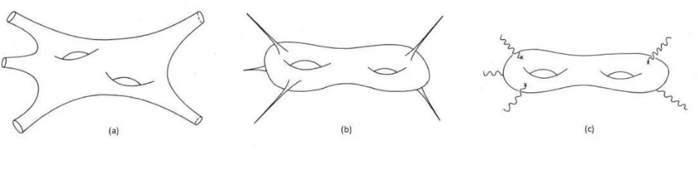
When calculating S-matrix withnexternal states, they are represented by the incoming and outgoing external handles of the surface (as it is shown in 1.1). For on-shell external states, the boundary of these handles can be set at large space-time distance (a). As we will see, the relevant structure of the surface for string theory is the conformal structure. This allows us to use a conformal map that locally acts asz =eς on the external handles,
transforming such world-sheet to a compact surface withnpoints removed (punctures)(b). Conversely, we can treat the worl-sheet as a compact surface without punctures but with local insertions of vertex operators which introduce the quantum numbers of the external states onto the surface (c). The relation between these two pictures will be revisited in section 2.5.
For a two dimensional manifold of genusg andnpunctures Σg,n, endowed with a metric
gab, in any local patch we can pick a complex parametrization z =σ1+iσ2, ¯z =σ1−iσ2
such that
ds2 = 2g
zz¯dzdz¯ (1.2)
It shows the residual symmetry due to conformal transformations: z → f(z) forf an an-alytic function. Therefore,gab determines a complex structure on Σg,ndefining a Riemann
surface.
Another metricg′
ab which is not related to gab by a globally defined diffeomorphism and
discontinuous reparametrizations called quasiconformal transformations. We will use this tool widely throughout the text.
After gauge-fixing the local symmetries, the Faddeev-Popov determinant is introduced into the functional integral. This determinant can be computed as an integral over Grass-mann ghost fields corresponding to variations of the gauge condition and to infinitesimal reparametrizations of the local coordinates. One may fix a covariant gauge which leaves conformal invariance as a residual symmetry. This remaining symmetry will be useful to study the local aspects of the theory. In this way, the operator product of the fields and the conformal algebra determine all the correlation functions of the theory.
The full action of the system which includes both the matter and the ghost actions, possesses a residual fermionic symmetry, the so called BRST symmetry. The BRST in-variance of string theory gives us an alternative approach to quantize the theory. The physical states are BRST invariant states modulo the null states. Moreover, BRST in-variance gives us useful information in order to build the covariant vertex operators which produce the physical states of the theory by acting on the ground state. Furthermore, BRST invariance is a powerful tool to study the unitarity of the scattering amplitudes, in particular the decoupling of non-physical states.
In order to successfully treat string theory as a conformal field theory, it must fulfil some important properties. On the one hand, all states in the two dimensional Hilbert space should have non-negative norm. What is more, negative norm states must decouple from scattering amplitudes in order to have a unitary time evolution as required by quantum mechanics.
On the other hand, the operator product of two fields, which produces their correspond-ing algebra, should be well-defined on the complex plane, which means that it should not change when any field is carried continuously around any point, which means that the correlation function must be single valued.
responsible for the absence of ultraviolet divergences.
Bosonic string theory can not represent a complete quantum model of nature because of two crucial aspects. Firstly, bosonic strings present a tachyon in their spectrum which is unacceptable for the stability of the theory. Furthermore, the spectrum only describes bosons and we need to come up with a novelty to include fermions if we desire a com-plete phenomenological description. This is solved by formulating a theory with local supersymmetry on the world-sheet (the Ramond-Neveu-Schwarz string).
In the same way conformal invariance was a remaining symmetry of the reparametriza-tion invariance in conformal gauge, superconformal invariance is the remaining symmetry of local supersymmetry in the superconformal gauge, for the fermionic string. Because of the boundary conditions of the two dimensional fermionic fields, the Hilbert space of a superconformal field theory split into two sectors, the Neveu-Schwarz (NS) and Ramond (R) sectors with periodic and anti periodic boundary conditions respectively.
We focus on the local properties of the superconformal structure of the superstring and on the calculation of tree amplitudes. The main issue is to obtain covariant vertex opera-tors which represent the fermionic and bosonic states of the theory. They are constructed from fields of the NS and R sectors which have the correct superconformal transforma-tions. The BRST symmetry plays a crucial role in order to construct the fermionic vertex operators. The Faddeev-Popov ghosts for local supersymmetry also enter in this con-struction in a essential way. Although the RNS string does not have manifest space-time supersymmety, we will see that a supersymmetric spectrum is required in order to have a consistent theory, free of anomalies. In particular, we will see that GSO projection, which yields a supersymmetric spectrum, is imposed by demanding modular invariance in loop diagrams.
The present text is organized as follows. Chapter 2 is devoted to the quantization of the bosonic string. Section 2.1 illustrates the basics of conformal field theory. In sections 2.2 and 2.3 we obtain the correct measure for the bosonic string in the critical dimension. The sections 2.4 and 2.5 are concerned with the BRST symmetry of the string in order to construct BRST invariant vertex operators. After an examination of the BRST invariance of the scattering amplitudes we examine the sources of possible anomalies. In section 2.6 we calculate explicitly the Virasoro-Shapiro amplitude and in the section 2.7 the bosonic amplitude is factorized isolating the divergence term. The one-loop partition function and the modular invariance of this amplitude is studied in section 2.8.
Quantization of the bosonic string
This chapter is devoted to study the quantization of the bosonic string and some of its most important properties as a two dimensional conformal field theory (CFT)[1][2] [3]. Treating string theory as a CFT on a Riemann surface is a natural formulation that will provide us with the necessary tools to implement the so called path integral quantization. For this reason, in the first section of this chapter, we review the basics of CFTs which will be widely used throughout this text.
2.1
Basics of two dimensional conformal field theory
2.1.1
Two dimensional conformal transformation
We consider a two-dimensional space M endowed with an Euclidean metric gµν. We
define a conformal transformation as a change of coordinates x → x′ such that it leaves
the metric invariant up to a scaling factor
gµν(x) = gµν′ (x′) =
∂ xα
∂ x′µ
∂ xβ
∂ x′νgαβ(x) = Ω(x)gµν(x). (2.1)
For the two dimensional case it is convenient to rewrite this in complex coordinates,
z =x1+ix2, ¯z =x1−ix2. Let us define the complex derivatives as
∂z =
1
2(∂x+i∂y), ∂¯z = 1
2(∂x−i∂y), (2.2)
in order to have ∂zz =∂¯zz¯= 1 and∂zz¯=∂¯zz = 0. 1
1Let us obtain the metric tensor in complex coordinates. We can see that g¯zz=gzz¯ = ∂zxµ∂zx¯ νgµν =∂zx1∂zx¯ 1+∂zx2∂zx¯ 2=
1 2.
The metric takes the form ds2 =dzdz¯. In this coordinate system, the condition (2.1)
consists of all transformations of the form 2
z → f(z), z¯→ f¯(¯z), (2.3)
where f and ¯f are arbitrary analytical functions. For these kind of transformations, the rescaling factor is Ω = |∂ f /∂ z|2. 3 The generators of infinitesimal conformal
trans-formations are 4
ln=−zn+1∂z l¯n=−z¯n+1∂¯z,
produce the infinite dimensional local algebra
[ln, lm] = (m−n)lm+n
¯
ln,¯lm
= (m−n)¯lm+n, (2.5)
and [ln,¯lm] = 0 .
There is an important point to remark about this algebra; the generators (2.5) are not well defined globally on the Riemann sphere S2 =C∪ ∞. 5
Demanding analyticity at z = 0, implies thatln is globally defined only for n≥ −1. In
order to describe the behaviour of functions atz → ∞ we make use of the inversion map
z =−1
u, (2.6)
In the same way, we can obtain thatgzz =g¯z¯z= 0. Thereforegzz¯=gzz¯ = 2.
2Letz′µ(z,z¯) be a reparametrization of the (z,z¯) coordinates. Then, in order this change of coordinates
to be a conformal transformation the components of the metric tensor must be g′
11 =g22′ = 0. We can
impose this condition, by using (2.1), getting the constraints
∂zz′1∂zz′2= 0, ∂ ¯ zz′1∂
¯
zz′2= 0.
The solution for this system isz′1=z′1(z) and z′2=z′2(¯z). The choice ofz1 or z2 is totally arbitrary.
Then, we see that the two-dimensional conformal transformations remains in analytical transformations of the form
z→ z′(z), z¯→z¯′(¯z). 3This follows fromds′2=|dz′
|2=|∂ z′
/∂ z|2|dz|2
4These generators expand the infinitesimal conformal transformationsz→ z+ǫ(z) and ¯z→ z¯+ ¯ǫ(¯z),
in the basis
and imposing analyticity for u= 0,
ln =−zn+1∂z =
−1u
n+1
1
u2
∂u =
−u1
n−1
∂u, (2.7)
it is easy to see that only the generatorsln, forn ≤ 0 are well defined atu= 0 and we note
the only conformal transformations defined globally are generated by {l0, l1, l−1} (global conformal transformations), producing translations l−1,¯l−1, dilations l0 + ¯l0, rotations i(l0 −¯l0) and special conformal transformations l1,¯l1. The finite form of this can be obtained from successive infinitesimal transformations and takes the form
z → az+b
cz+d, ad−bc= 1, a, b, c, d ∈ C. (2.8)
This is the SL(2,C) group of transformations. The transformation above remains
unaltered when changing the sign of all the coefficients, a, b, c and d, and we need to incorporate a quotient of Z2. These group of transformation is known as the group of
projective conformal transformationsSL(2,C)/Z2.
Moreover, since the total algebra is the direct sum of the holomorphic and anti-holomorphic algebra (2.5), the variables z and ¯z can be treated as independent coordinates. The phys-ical condition z∗ = ¯z is left to be imposed at some convenient point.
2.1.2
Conformal fields in two dimensions
From now on, we shall generalize the above ideas to the quantum realization of the conformal algebra. In order to define a field theory with conformal invariance we require a set of fields {Aj}, in general infinite, which includes the derivatives of all the fields Aj.
The complete set of states of the theory can be obtained by the action of the conformal fields on the ground state. 6 The vacuum |0i, by definition, is invariant under the action
of the global conformal groupSL(2,C) invariant). There is a subset of fields{φj}, called
quasi-primaries, which under global conformal transformations x→ x′ transform as
φi(x)→
∂ x
′
∂ x
di/2
φi(x′), (2.9)
6This is an important fact of conformal field theories quantized on a circle, namely, the state-operator
correspondence. An asymptotic state propagating from τ → −∞ can be conformally mapped to the origin by using a map that locally acts asew (wherew=τ+iσ). This map defines a local operator at
where di is the scaling dimension ofφi. 7
We can obtain the total set of fields by linear combinations of the elements of{φi}and
their derivatives.
The correlation functions of quasi-primary fields transform according to
hφ1(x1). . . φn(xn)i=
∂ x ′ ∂ x
d1/2
x=x1
. . . ∂ x ′ ∂ x
dn/2
x=xn
hφ1(x′1). . . φn(x′n)i. (2.11)
Conformal invariance imposes strong constraints on the correlator functions of quasi-primary fields, specially for the two and three point functions. According to (2.11), the 2-point function correlator must transforms as
G(x1, x2) = hφ1(x1)φ2(x2)i= ∂ x ′ ∂ x
d1/2
x=x1
∂ x ′ ∂ x
d2/2
x=x2
hφ1(x′1)φ2(x′2)i. (2.12) Invariance under translations and rotations requires that
G(x1, x2)≡G(|x1−x2|), (2.13) and transformation by dilationsx′ =λ x tell us that
G(|x1−x2|) = λd1+d2G(λ
|x1−x2|), (2.14)
which implies
G(|x1−x2|) = C12
|x1−x2|d1+d2
. (2.15)
Finally, special conformal transformation which are given by
x′ = x+bx2
1 + 2b˙x+b2x2 , (2.16)
forces thatd1 =d2 in order to have a non-zero correlator, thus
hφ1(x1)φ2(x2)i=
C12
|x1−x2|2d for d1 =d2 =d
0 for d1 6= d2 . (2.17)
The three-point function can be obtained in a similar way
hφ1(x1)φ2(x2)φ3(x3)i= C123
|x1−x2|d1+d2−d3
|x2 −x3|d2+d3−d1
|x1−x3|d1+d3−d2 , (2.18)
7The scaling dimension ofφdefines the transformation of the field under a rescaling of coordinates.
On the other hand, there is a subset of quasi-primary fields {Φi(z,z¯)} which, under the
conformal mapz → w=f(z), transforms as
Φ′(z,z¯) = (∂ w
∂ z)
h(∂w¯
∂z¯)
¯
hΦ
i(f(z),f¯(¯z)), (2.19)
these fields are called (h,¯h) primary fields, where h and ¯h are defined as the holomor-phic and anti-holomorholomor-phic conformal dimensions of Φ which are related to the scaling dimension d and the planar spin s as 8
h+ ¯h=d , h−¯h=s , (2.20)
We remark that transformations of the form w=f(z) are not restricted to global confor-mal transformationsSL(2,C), but to any conformal transformation. Under an
infinitesi-mal coordinate transformation z → z+ǫ(z), (2.19) gives
δΦ(z,z¯) = (h∂ǫ+ǫ∂+ ¯h∂¯ǫ¯+ ¯ǫ∂¯) Φ(z,z¯). (2.21)
2.1.3
Energy-momentum tensor
The energy-momentum tensorTαβ is a (2,2) quasi-primary field (SL(2,Z) primary) which
plays a central role in conformal field theory. For a two-dimensional field theory defined by an actionS(φi, gα,β) we define the symmetric tensor Tαβ as
Tαβ = −
2π
√g δ S(δ gφiαβ, gαβ). (2.22)
For an action invariant under Weyl transformations gαβ → gαβ′ = Ωgαβ, the
energy-momentum tensor is traceless, that is 9
0 = −√2π
g
δ S(φi, gαβ)
δΩ =
−2π
√g δ S φi, g
′
αβ
δ g′αβ
δ g′αβ
δΩ =T
α
α . (2.23)
In order to rewrite this expression in complex coordinates, we use tensor transformations
8These values will be defined below as the eigenvalues of the operators of dilation and rotationL 0+ ¯L0
andL0−L¯0 respectively.
9Taking into account thatS(φi, gαβ) =S(φi, g′
and calculate10
Tzz¯ = ∂σα
∂z ∂σβ
∂z¯ Tαβ
= ∂σ
1 ∂z
∂σ1 ∂z¯T11+
∂σ2 ∂z
∂σ1 ∂z¯T21+
∂σ1 ∂z
∂σ2 ∂z¯T12+
∂σ2 ∂z
∂σ2 ∂z¯T22
= 1
4(T11+T22) = 0. (2.24)
Let us consider that the actionS(φi, gα,β) possess conformal invariant. Letǫα be a vector
field generating translations of the formσα →σα+ǫα, then
0 = δǫS(φi, gαβ)
= Z
d2σ
δ S δ gαβδǫg
αβ +δ S
δφδǫφ
= 1
2π
Z
d2σ√g Tαβ(∇αǫβ+∇βǫα), (2.25)
where in the second line we made use of the equation of motion of φ. After integrating by parts we obtain the conservation law of the energy-momentum tensor.
∇αTαβ = 0. (2.26)
The last result together with (2.24) can be used to show that
∂¯zTzz = 0, ∂zT¯zz¯= 0. (2.27)
Then, the two remaining non-zero components of the the energy-momentum tensor are the holomorphic Tzz =T(z) and the anti-holomorphic T¯z¯z = ¯T(¯z) components.
In general, (anti)holomorphic fields O(z) of weight h (¯h) can be expanded in Laurent series as follows
O(z) =
∞
X
n=−∞
On
zn+h, O¯(¯z) =
∞
X
n=−∞
¯
On
¯
zn+¯h . (2.28)
The Laurent modes satisfy
On =
1 2iπ
I
dz zn+h−1O(z). (2.29)
10You should note that we renamed thexcoordinates asσ. We leavexto label the matter field system
The components of the energy-momentum tensor Tzz and Tz¯z¯ have weights (2,0) and
(0,2) respectively. This is obtained by a rescaling z → λ z . Then, components of the energy-momentum tensor has the Laurent expansions
T(z) =
∞
X
n=−∞ Ln
zn+2, T¯(¯z) = ∞
X
n=−∞
¯
Ln
¯
zn+2 . (2.30)
We have obtained the energy-momentum tensor as a conserved charge due to two-dimensional translations, therefore Tαβ is the generator of these variations but not conformal
formations. We need to introduce a conserved current associated with conformal trans-formations. Given a vector fieldvα, let us consider
Jα =vβTαβ. (2.31)
We note that a vector field vα produces a change in the metric of the form
δvgαβ = ∇αvβ+∇βvα = (P1v)αβ+ (∇.v)gαβ,
(P1v)αβ = ∇αvβ+∇βvα−(∇.v)gαβ (2.32)
The value of (P1v)αβ is only zero if vα is a conformal Killing vector(CKV), leaving
invariant the metric up to a scaling factor. It follows that
∇αJα = ∇α(vβTαβ)
= (∇αTαβ)vβ+ (∇αvβ)Tαβ
= 1
2(∇αvβ+∇βvα)T
αβ (2.33)
where we have used the conservation and symmetry of the energy-momentum tensor. Now, if the reparametrization σα → σα+vα is a conformal transformation, it follows
that
∇αJα =
1 2(∇ρv
ρ)g
αβTαβ = 0. (2.34)
We expect this quantity to be the conserved charge which produces conformal transfor-mations.
2.1.4
Radial quantization
Until now we have been considering complex coordinates of the form ς ,ς¯=σ1 ± iσ2
for the two dimensional euclidean time σ1 and space σ2. This define a cylinder after
considering the spatial coordinate periodic σ2 ≡ σ2+ 2π. The conformal transformation
maps the cylinder to the complex plane whose origin (z = 0) is related to the distant past (σ1 → −∞). The euclidean time points radially outward from the origin; that is
the reason why quantum version of the dilation operator in the complex plane, namely,
L0+ ¯L0, is considered as the Hamiltonian. The charge associated with Jα can be written
using complex coordinates as follows
Q = 1
2π i
I
C
dzαTαβǫβ
= 1
2π i
I
C
dz T(z)ǫ(z) +dz¯T¯(¯z)¯ǫ(¯z) . (2.36)
whereC is a contour that surrounds the origin. This conserved charge produces conformal transformations on the fields φ(w,w¯) in the following way
δφ(w,w¯) = [Q, φ(w,w¯)] = 1 2π i
I
C
dz [T(z)ǫ(z), φ(w,w¯)]+ 1 2π i
I
C
dz¯T¯(¯z)¯ǫ(¯z), φ(w,w¯) .
(2.37) After being compactified σ2 direction, we choose the σ1 direction as the quantization
direction. In the complex plane this means that the operators must be radially ordered. The prescription for radial ordering is
R(A(z)B(w)) :=
A(z)B(w) for |z|>|w|
B(w)A(z) for |w|>|z| . (2.38)
Taking this into account, conformal field transformations (2.37) can be expressed as (holo-morphic part)
I
|z|>|w|
dz T(z)ǫ(z)φ(w,w¯)− I
|z|<|w|
dzφ(w,w¯)T(z)ǫ(z)
= I
C(w)
dzR(T(z)ǫ(z)φ(w)). (2.39)
We have to keep in mind thatT(z) is analytic everywhere except at the point where φ
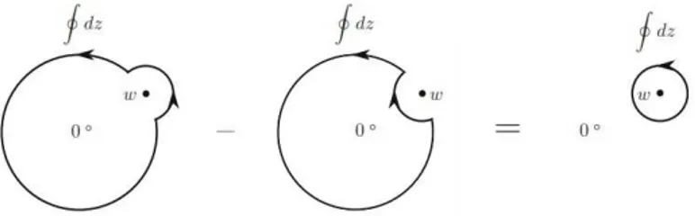
is inserted, this allows us to deform the contour into a small circle surrounding w (figure 2.1).
Figure 2.1: Contour of integration
characterized by their Operator Product Expansion (OPE).
Ai(z)Bj(w)∼
X
k
ckij(z−w)Ok(w), (2.40)
where {Ok}is a complete set of local operators and ckij are singular coefficients.
The singular part of the OPE between T(z) and φ(w,w¯) can be easily obtained by comparing equations (2.39) and (2.21), and can be written as
T(z)φ(w,w¯) ∼ h
(z−w)2 φ(w,w¯) +
1
z−w∂wφ(w,w¯) (2.41)
¯
T(¯z)φ(w,w¯) ∼ ¯h
(¯z−w¯)2 φ(w,w¯) +
1 ¯
z−w¯∂w¯φ(w,w¯). (2.42)
2.1.5
Central charge and Virasoro algebra
The variation of the energy-momentum tensor can be expressed as a linear function of
T and their derivatives. Following [5] wee write the expression for the variation δ T(z) under infinitesimal conformal transformation11
δT(w) = c 12∂
3ǫ(w) + 2∂
wǫ(w)T(w) +ǫ(w)∂wT(w), (2.43)
11The most general expression for this variation should include a second derivative term, however the
the factor c
12 has been chosen for convenience.
12 This variation, as stated in the discussion
above, is produced by action of (2.36) on T(w)
δT(w) = 1 2π i
I
Cw
dz ǫ(z)T(z)T(w),
then we see that (2.43) holds if the OPE T(z)T(w) is given by
T(z)T(w)∼ c/2 (z−w)4 +
2T(w) (z−w)2 +
∂T(w)
(z−w). (2.45)
At this point it is instructive to say that the OPE of two arbitrary fieldsA(z1)B(z2) must
be symmetric in z1 and z2 [6]. This explains why terms with second order derivatives in
ǫ(w) does not appear in δ T(w). The same considerations apply for the anti-holomorphic component
¯
T(¯z) ¯T( ¯w)∼ ¯c/2 (¯z−w¯)4 +
2 ¯T( ¯w) (¯z−w¯)2 +
¯
∂T¯( ¯w)
(¯z−w¯). (2.46)
By treatingT(z) as an operator, the Laurent modes are promoted to operators too. Their algebra can be obtained by application of radial ordering and using the OPE (2.45). The modes Ln of energy-momentum tensor are
Ln=
I dz 2iπT(z)z
n+1, (2.47)
considering the discussion above we obtain the algebra
[Ln, Lm] =
I C0 dw 2iπ I Cw dz
2iπw
n+1zm+1
R(T(z)T(w))
= I C0 dw 2iπ I Cw dz
2iπw
n+1zm+1( c/2
(z−w)4 +
2T(w) (z−w)2 +
∂T(w) (z−w)) =
I
C0
dw
2iπw
n+1 c
12(m+ 1)m(m−1)w
m−2+ 2(m+ 1)wmT(w) +wm+1∂
wT(w)
.
(2.48)
12As we will see, the energy-momentum tensor is not a primary field beacause it does not transform
as (2.19), but a quasi-primary field, namely, a SL(2,C) primary. Equation (2.43) corresponds to the
transformation under finite conformal transformation (2.157)
T(z)→ T′(f(z)) =
df(z)
dz
−2
T(z)−12c {f(z);z},
where the term{f(z);z}is the Schwartzian derivative
{f(z);z}= d
3f(z)/dz3 df(z)/dz −
3 2
d2f(z)/dz2 df(z)/dz
2
After integration onw and considering (2.47) we get [Ln, Lm] = (m−n)Lm+n+
c
12(m
3
−m)δm+n. (2.49)
The ¯Ln modes satisfy the same algebra and Lm commutes with ¯Ln. This is the Virasoro
algebra. It is essential to remark that every conformal field theory defines a representation of this algebra, characterized by the central chargec. On the other hand, global conformal transformationsSL(2,C) generated by L−1,0,1 and ¯L−1,0,1 form a subalgebra without the
anomalous term c(2.5).
The effect ofLn on the vacuum can be determined as follows
Ln|0i ∼=
Z
dz
2iπz
n+1T(z)
|0i . (2.50)
By requiring the regularity of T(z), the integral vanishes for n > −1. We state this important result as
Ln|0i= 0, n > −1 (2.51)
To define h0| at z → ∞, we use the same reasoning but now for the map u =−1/z and demanding regularity at u= 0. Similarly, we obtain for out-states
h0|L−n, n >1. (2.52)
The generators L1,0,−1 and ¯L1,0,−1 annihilates both |0i and h0|, which means that the
vacuum is SL(2,C) invariant. The same applies for ¯Ln.
2.1.6
Highest weight states and descendant fields
In a conformal field theory quantized on a circle, there is an important isomorphism between the set of local operators and the space of states of the theory. For an S-matrix calculation, one must specify initial and final states. Initial states (σ0 → −∞) can be
created by a field acting on the vacuum. On the complex plane this means to insert a local operator at the origin z = 0
|φi ≡φ(z = 0)|0i . (2.53)
Let φ be a primary field. By using the OPE with the energy-momentum tensor we can obtain the commutator of the modes Ln with φ
[Ln, φ(0)] =
I
dz
2iπz
n+1T(z)φ(w)
= I
dz
2iπ(hz
we easily see that for n > 0 the integrand is holomorphic at z = 0, as a consequence the integral vanishes. However, for n = 0 we have a single pole which yields to a non zero answer. Taking into account that Ln annihilates the vacuum for n > −1, we can
summarize
Ln|φi=
0 for n≥ 1,
h|φi for n = 0 . (2.55)
States satisfying this condition are known as the highest weight states. Furthermore, noting that [L0, Ln] = −nLn we see that for n > 0, the action of Ln on φ|0i lowers its
weight by n. States of the form
Lin
−n...L i2
−2L
i1
−1|φi (2.56)
are known as descendant states. We note that every primary field gives rise to an infinite set of descendant fields. In this sense, Virasoro algebra organizes the fields of a conformal field theory by grouping them in families, each of these, labelled by a primary field. For bosonic strings, there are two important conformal systems to take into consideration; the ghost systembc and the matter system xµ.
2.1.7
Matter system
Our principal motivation in this chapter is to obtain the quantization of the Polyakov action (1.1). After fixing the conformal gauge, it means, ˆgab =eφ(σ1,σ2)δab, we have to deal
with the conformal symmetry which remains unfixed. The gauge fixed Polyakov action can be written as 13
S = 1 2πα′
Z
d2z ∂zxµ∂¯zxµ, (2.57)
with equations of motion
∂z(∂z¯xµ) = ∂z¯(∂zxµ) = 0. (2.58)
We can see that ∂xµ and ¯∂xµ are holomorphic and antiholomorphic fields of weight
13After fixing the conformal gauge in Polyakov’s action, we can rewrite this in complex coordinates by
considering the non-zero components of the metric tensor ˆg¯zz= ˆgzz¯= e
φ(z,z¯) 2 and ˆg
¯
zz= ˆgzz¯= 2e−φ(z,¯z).
Now, it is easy too see that ˆ
g1/2d2σ=eφ(z,¯z)dzdz¯
2 , ˆg
(1,0) and (0,1) respectively, and have Laurent expansions of the form
∂zxµ(z) =−i
r α′ 2 ∞ X n=−∞ αµ n
zn+1, ∂¯zx
µ(¯z) =
−i r α′ 2 ∞ X n=−∞ ¯ αµ n ¯
zn+1 (2.59)
Thus, the mode expansion for xµ(z,z¯) split into a sum of holomorphic and
antiholo-morphic part and is obtained by integrating (2.59)
xµ(z,z¯) =xµ(z) +xµ(¯z) (2.60)
xµ(z) = x
µ
0
2 −i
α′
2p
µlnz+i
r α′ 2 ∞ X n=−∞ αµ n n z −n,
xµ(¯z) = x
µ
0
2 −i
α′
2p
µln ¯z+i
r α′ 2 ∞ X n=−∞ ¯ αµ n
n z¯
−n, (2.61)
here, xµ0 and pµ = 2
α′
1/2
α0 = α2′
1/2
¯
α0, represent the center of mass-momentum posi-tion and momentum of the string. The algebra generated by these modes can be obtained by using the propagator of the matter system. We obtain this by following [4], 14
0 = Z
Dx δ
δxµ(z,z¯)
[exp (−S)xν(w,w¯)]
= Z
Dx exp (−S)
ηµνδ2(z−w,z¯−w¯) + 1
πα′ ∂z∂¯zx
µ(z,z¯)xν(w,w¯)
= ηµνδ2(z−w,z¯−w¯)+ 1
πα′ ∂z∂¯zhx
µ(z,z¯)xν(w,w¯)
i , (2.62)
which holds as an operator equation. Solving (2.62) we get
hxµ(z,z¯)xν(w,w¯)i=−ηµνα ′
2 ln|z−w|
2. (2.63)
where we have made use of the identity
∂z∂¯zln|z|2 =∂¯z
1
z = 2π δ
2(z,z¯). (2.64)
This result will be useful as the starting point to define the conformal normal ordering
of an operator. The conformal normal ordering of a field O is obtained by subtracting all
self contractions. For the matter field xµ we have that
:xµ(z,z¯) : = xµ(z,z¯), (2.65)
:xµ(z,z¯)xν(w,w¯) : = xµ(z,z¯)xν(w,w¯)− hxµ(z,z¯)xν(w,w¯)i = xµ(z,z¯)xν(w,w¯) + α
′
2 η
µνln
|z−w|2. (2.66) As we will use frequently in this text, we obtain the energy-momentum tensor for the matter system by the Noether method. The energy-momentum tensor is the conserved charge related to symmetry under translations δz = ǫ , δz¯ = ¯ǫ. Under this variations, matter fields transform as δxµ(z,z¯) = ǫ ∂
zxµ+ ¯ǫ ∂¯zxµ and varying the action
δS = 1 2πα′
Z
d2z
−:∂zxµ∂zxµ :∂¯zǫ−:∂¯zxµ∂¯zxµ :∂z¯ǫ+
+∂z(∂¯zxµ∂zxµǫ) +∂¯z(∂zxµ∂¯zxµǫ¯)
. (2.67)
The last two terms are total derivatives and can be dropped, and we obtain the energy-momentum tensor which splits in holomorphic and antiholomorphic components, as ex-pected
15
T(z) = −1
α :∂zx
µ∂
zxµ:, T¯(¯z) = −
1
α :∂¯zx
µ∂¯
zxµ: . (2.72)
15In particular, we can obtain the transformation law (2.120) forT(z) =−1
α :∂zxµ∂zxµ: by rewriting
it as
T(z) = lim
ǫ→0
−α1 ∂zxµ(z+ǫ)∂zxµ+ 1
αh∂zx
µ(z+ǫ) ∂zxµi
(2.68) Let us consider two pointsz1andz2such thatz1−z2=ǫ. For a conformal transformationz→ f(z) we
see thatf(z1)−f(z2) =η. We are concerned with the variation of the singular part
1
αh∂zx
µ(z+ǫ)∂zxµi = f′
(z+ǫ)f′
(z)1
α
−α D/2 (f(z+ǫ)−f(z))2
= f′(z)
f′(z) +ǫ f′′(z) +ǫ
2
2f
′′′
(z)
−D2 1
(ǫ f′(z) +ǫ2 2f
′′(z) +ǫ3 6f
′′′(z))2 !
= −D2f′
(z)
f′
(z) +ǫ f′′
(z) +ǫ
2
2f
′′′
(z)
1 + ǫ
2 f′′(z)
f′ +
ǫ2 6
f′′′(z)
f′(z) −2
ǫ2f′(z)2 ,
(2.69) expanding the polynomial and taking the limitǫ→ 0 we get
1
αǫlim→0h∂zx
µ(z+ǫ)∂zxµi=−lim ǫ→0
D/2
ǫ2 =−ηlim→0(f
′
(z))2
D/2
η2
− D
12
f′′′(z)f′(z) +f′′(z)2 f′(z)2
And the commutation relation of the mode expansion (2.61) are given by
[αµm, ανn] = [¯αµm,α¯νn] =mδm+nηµν,
[xµ, pν] = iηµν. (2.73)
The representation for this algebra can be constructed by defining a ground state with momentum kµ, |0, ki that are annihilated by lowering operators, that is, all the modes
αµ
n with n >0. The complete Hilbert space of the theory is obtained by acting with the
raising operators, the modes αµ
n with n <0, on the ground state.
2.1.8
Ghost system
We consider two holomorphic anti-commutating fields b and c with conformal weights (λ,0) and (1−λ,0) with the following action
Sg =
1 2π
Z
d2z b ∂¯zc . (2.74)
We can see that the action is invariant under conformal transformations. The equations of motion for the fields of this system are given by
¯
∂b= ¯∂c= 0. (2.75)
These equations tell us that the fields we are considering are indeed holomorphic, so we can now write down how they transform under infinitesimal conformal transformations.
δb(z) = λ ∂zǫ b(z) +ǫ ∂zb(z), (2.76)
δc(z) = (1−λ)∂zǫ c(z) +ǫ ∂zc(z). (2.77)
obtain the variation ofT(z)
T(z)→f′′
(z)T(f(z)) + D 12
f′′′
(z)f′
(z) +f′′
(z)2 f′(z)2
We can use these transformations to apply Noether’s procedure in order to find the energy-momentum tensor of the ghost system
δSg =
1 2π
Z
d2z[δb ∂¯zc+b ∂¯zδc]
= 1
2π
Z
d2z [(λ ∂zǫ b+ǫ ∂zb)∂¯zc+b ∂¯z((1−λ)∂zǫc+ǫ ∂zc)]
= 1
2π
Z
d2z [b(1−λ)∂z∂¯zǫ c+ ¯ǫ b∂zc]
= −1 2π
Z
d2z[(1−λ)∂zb c−λ b ∂zc]∂¯zǫ . (2.78)
hence,
Tg(z) = (1−λ) :∂b c:−λ:b ∂c: , (2.79) We calculate the propagator for the bc CFT in order to compute relevant OPE’s by proceeding as we did for the matter system .
0 = δ
δc(z) Z
DbDc[exp(−Sg)c(w)]
= Z
DbDcexp(−Sg)
− 1
2π∂¯zb(z)c(w) +δ 2(z
−w,z¯−w¯)
. (2.80) Since the equations above hold inside path integrals, we can write them as operator equations,
∂¯zhb(z)c(w)i= 2πδ2(z−w,z¯−w¯). (2.81)
Solving the equation above, we find the propagator for the bcCFT which is given by
hb(z)c(w)i= 1
z−w. (2.82)
Now, it is straightforward to obtain the OPEs of Tg with the ghost fields
Tg(z)c(w)∼(1−λ) c(w) (z−w)2 +
∂c(w)
(z−w), (2.83)
Tg(z)b(w)∼λ b(w)
(z−w)2 +
∂b(w)
(z−w), (2.84)
and the Laurent expansions of the ghost fields
b(z) =
∞
X
m=−∞ bm
zm+λ , c(z) =
∞
X
m=−∞ cm
These modes satisfy
bn =
I dz 2iπz
n+1b(z), c
n=
I dz 2iπz
n−2c(z). (2.86)
By imposing analyticity on the SL(2,C) invariant ghost vacuum |0ibc, the oscillators act
as
bn|0ibc = 0 for n ≥ −1,
cn|0ibc = 0 for n ≥2. (2.87)
On the other hand, the algebra of the bc system can be obtained from the propagator (2.81)
{bm, cn}=δm,−n. (2.88)
We note that the zero modes b0, c0 satisfy the anti-commutation relations
{b0, c0}= 1, b20 =c20 = 0, (2.89) and they commute with the Hamiltonian Lg016, therefore we have a degenerate ground
state |↓i and |↑i satisfying
b0 |↓i = 0, b0 |↑i=|↓i, (2.91)
c0 |↓i = |↑i, c0 |↑i= 0, (2.92)
bn |↓i = bn|↑i=cn |↓i=cn|↑i= 0, n >0. (2.93)
The total spectrum is obtained by acting on theses states with the negative modes of the ghost fields. It is worthwhile noting that instead|0ibc is the ground state of the Virasoro
16It clearly follows from the definition of the Virasoro modes (2.47). Explicitly, the commutation with
thec0 mode
[Lg0, c0] = I
Cw
dz
2iπz
I
C0
dw
2iπw
−λ
(1−λ) c(w) (z−w)2 +
∂c(w) (z−w)
=
I
C0
dw
2iπ (1−λ)c(w)w
−λ+∂c(w)w1−λ
=
I
C0
dw
2iπ (1−λ)c(w)w
−λ
−(1−λ)c(w)w−λ= 0
algebra, it is not the highest weight state of the bc algebra since it is not annihilated by all the the positive modes. It can be cured by noting that b−1 |↓i satisfies (2.87), thus
|0ibc=b−1 |↓i (2.94)
It follows that c1|0ibc =c1b−1 |↓i=|↓i+b−1c1 |↓i, and|↓i can be represented by
|↓i=c1|0ibc (2.95)
and
|↑i=c0c1|0ibc (2.96)
Further, we can note that h↓|↓i= 0 by inserting the commutator (2.89) equal to 1
h↓|↓i=h0|c−1(b0c0+b0c0)c1|0ibc= 0 (2.97)
because ofb0annihilates bothSL(2,C) vacua. We can obtain the same result forh↑|↑i= 0.
However, the value of h↓|↑i is different to zero and can be normalized such that
h0|c−1c0c1|0ibc= 1 (2.98)
In this sense, c−1c0 is the dual of c1.
2.2
Path integral quantization
The evolution of a string generates a two dimensional surface, which is known as the world-sheet, embedded in a target space. The incoming and outgoing strings indicate the merging of initial and the emergence of final states, possibly accompanied by creation and annihilation of virtual string pairs. By using conformal transformations, such a world-sheet can be mapped to a compact surface with a number n of points removed which correspond to external string states (punctures). The path integral quantization is performed by summing in the functional integral over all compact surfaces (Polyakov path integral)[7].
As it is well known, this integration contains an overcounting due to summation over configurations that are related by local symmetries of the action. We will solve this difficulty by calculating the correct integration measure on a particular slice, it means, by using the well known Faddeev-Popov method[8].
physical states and the amplitudes of the theory. For standard references see [4] [9]. The main objective of this section will be to quantize the Polyakov’s action by the path integral method.
S = 1 4πα′
Z
Σg
d2σ√ggab∂axµ∂bxµ (2.99)
where Σg is a Riemann surface with genus g. In this approach we consider as the
two-dimensional quantum fields the embedding xµ(σ1, σ2) in the Minkowski spacetime and
the euclidean metric of the world-sheet gab(σ1, σ2). The functional integral is computed
by integrating over them. As we said, this summation is overvalueted because of local world-sheet symmetries of the action:
2.2.1
Classical local symmetries of the Polyakov’s action
The Polyakov’s action has the following world-sheet symmetries: 1)Diffeomorphism invariance
σa→σ′a(σa), gab(σ)→gab′ (σ′) =
∂ σc
∂ σ′a
∂σd
∂σ′bgcd(σ). (2.100)
2)Weyl invariance
σa→σa, gab(σ)→Ω(σ)gab(σ), (2.101)
Also, the Polyakov’s action is invariant under D-dimensional Poincar´e transformation
xµ→x′µ = Λµνxν +aµ, (2.102)
whit Λµ
νa Lorentz transformation and aµ a translation. We have to note that
diffeomor-phism generated by continue vector fields: σ′a =σa+va form a subgroup of
transforma-tions, Diff0, which produces the infinitesimal variation:
δ xµ=va∂axµ, δ gab=∇avb+∇bva. (2.103)
It is important to remark that a subgroup of diffeomorphisms does leave invariant the metric tensor up to a rescaling factor, producing a conformal transformation. This extra symmetry is still preserved after fixing the gauge (Conformal Symmetry).
2.2.2
The S-matrix
The on-shell scattering amplitude is given by
< Vk1, ..., Vkn >=
∞
X
h=0
Z
DgabDxµ
N e −S
n
Y
i=1
In order to obtain the correct measure, we have divided the functional integral by the volume of the local symmetry group, N = V ol(Diff⊗Weyl). The product of n Vertex Operators Vi, represent incoming or outgoing strings joining on the world-sheet. Vertex
operators for on-shell physical states must accomplish the symmetries of the full theory. In particular, Poincar´e invariance give us crucial information in their construction. Space-time translation invariance requires that the xµ dependence appears as an exponential
factor eikµxµ and its derivatives. On the other hand, Lorentz invariance requires that
all the space-time indices must be contracted with a polarization tensor. Then, vertex operators are of the form
Vi(ki, xµ) = P(ξ , Dxµ)eik.x (2.105)
whereξis the polarization vector andP(ξ , Dxµ) is a polynomial expression in the
deriva-tives ofxµ. We will say more about vertex operators in section 2.5. The total actionS is
defined as
S =SP +λχ , χ=
1 4π
Z
Σg
d2σ√gR , (2.106)
whereλ is a coupling constant and χis a diffeomorphism and Weyl invariant term which in two dimensions corresponds to the Euler number,χ= 2−2g−b for compact surfaces with genus g and b boundaries. Adding external string states corresponds to reduce the Euler number by 1, so the closed string coupling constant gc should be proportional to
eλ. The functional measure Dxµ and Dg
ab are defined by the inner product
hδ x, δ xi = Z
d2σ√gδ xµδ xµ
hδ g, δ gi = Z
d2σ√ggacgbdδ gabδ gcd. (2.107)
The factorN =V ol(Diff⊗Weyl) in the functional integral can be removed by restricting the integral to a gauge slice. The metricgab, as a symmetric tensor, possesses three degrees
of freedom. On the other hand, there are three gauge functions, two reparametrizations and the local scaling of the metric, which are enough gauge freedom to fix the metric to a c-number and forget the integration over the metric. However, the Weyl scaling is a genuine symmetry of the classical action, we will see that quantum mechanically it is lost unless we fix the space-time dimension to 26. Nevertheless we can bring the metric locally to a flat metric in 26 dimensions, it is not correct globally if we are interested to describe surfaces with Euler characteristic different to zero. A convenient choice is to consider the effect of the diffeomorphism group alone and fix the metric to the unit form up to a Weyl rescaling. A good slice is the conformal class [ˆg] of metrics conformal to some metric ˆgab
As we will see below, for surfaces with genus g >0 one conformal class is not enough to obtain a correct global gauge slice. These inequivalent conformal classes [ˆgab(m1...mk)]
are parametrized by a finite number of variables {mi} called the moduli. This implies
that any metric can be reached by the action of the local group of symmetries over the elements of the equivalence class [10]
gab′ (σ′, m1, ..., mk) = exp(φ(σ))
∂ σc
∂ σ′a
∂σd
∂σ′bˆgcd(σ, m1, ..., mk) (2.109)
Infinitesimal variations of the metric by Weyl and diffeomorphism transformations are given by
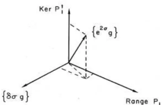
δ gab =δφ(σ)ˆgab+∇avb +∇bva.
These two variations are not orthogonal between them. As we said, they are related by the subgroup of conformal transformation. In order to factorize this, we split it in two orthogonal components, trace and traceless variations:
δ gab = ˜φ(σ)ˆgab+P1(v)ab
P1(v)ab =∇avb+∇bva−(∇.v)ˆgab φ˜(σ) = δφ(σ) + (∇.v))ˆgab
These variations are associated with the symmetries of the action, this means, they con-nect configurations representing the same physical system. Furthermore, we can see there exist a variation δ g∗ on the metric space which is orthogonal to variations by Weyl and
diffeomorphism
hδ g∗, δ gi = hδ g∗, P1(v)abi+hδ g∗,φ˜(σ)i (2.110)
= hP1†δ g∗, vi= 0 (2.111)
then we can see by using (2.107) that (P1†δ g∗)
a =−2∇bδ gab∗ . In order to have an
orthog-onal transformation between Image of P1 and δ g∗
ab, it must belong to theKerP
† 1:
∇bδ gab∗ = 0 (2.112)
These elements are called quadratic differentials. For the case of complex coordinates, quadratic differentials can be represented by (2,0) and (0,2) forms deforming the metric as
φzzdzdz+ ¯φz¯z¯dzd¯ z¯ (2.113)
such that∂¯zφzz =∂zφ¯¯z¯z = 0, the so-called (anti)holomorphic quadratic differential which
Figure 2.2: Orthogonal descomposition ofe2σˆg
the other hand, diffeomorphisms of vector fields that fall in the KerP1 are responsible for the extra symmetry, which still remains after fixing the gauge
∇avb +∇bva= (∇.v)ˆgab (2.114)
This means that any deformation of the metric can be factorized as
{δ gab}={δ φ gab}+{RangeP1}+{KerP1†} (2.115)
The first two terms on the right hand side consist of modes that can be gauged away. Let us explain this better by definingMg, the space of all the metrics defined on Σg, in which
we are integrating. However, as we have seen, the integral should be factorized by the volume of the gauge group N =V ol(Diff0(Σg)⊗Weyl(Σg)), restricting the integral over
deformations produced by the quadratic differentials. As we shall see in the next section, the Riemann-Roch theorem restricts the dimension of KerP1† by
dimKerP1†=
0 h= 0
2 h= 1
6h−6 h≥ 2
(2.116)
So, we expect to reduce the functional integral to finite-dimensional integrals in every loop expansion. In order to get more insight into the nature of the metric space Mh, in
which we are performing the functional integral, we define the Teichmuller Space as
Th =
Mh
Diff0(Σg)⊗Weyl(Σg)
(2.117)
mi forh equal to 0, 1 and≥ 2 respectively. Then, every variation in the Metric Space are
of the form δ mi∂
igab (irunning on the moduli coordinates). However, we do not want to
gauge away only Diff0(Σg) but Diff. We define the Mapping Class Group,
M CG= Dif f(Σg)
Dif f0(Σg)
. (2.118)
as the subgroup of diffeomorphisms not connected to the Identity. The space in which we are interested is Moduli Space Mh and defined as
Mh =
Th
M CG (2.119)
It is worthwhile to introduce the dual space to quadratic differentials. An arbitrary metric of a Riemann surface can be represented on a coordinate neighbourhood U(x, y) by
ds2 =A(x, y)dx2+B(x, y)dxdy+C(x, y)dy2,
here, A, B and C are functions of x and y. Using complex coordinates, it takes the following form
ds2 =λ(z,z¯)|dz+µ dz¯|2 (2.120) whereλis a positive smooth function onU. On the other hand, it is known from Riemann theorem that, at least locally, we can obtain coordinate system (w,w¯) in which the metric
ds2 can be written in isothermal form, ˜λdwdw¯. Rewriting this in z language we have that ds2 = ˜λ|dw|2 = |∂zw dz+∂¯zw dz¯|2 (2.121)
= ˜λ|∂zw|2
dz+ ∂¯∂zzwwdz¯
2
(2.122)
= ˜λ|∂zw|2|dz+µzz¯dz¯| 2
(2.123)
We conclude that if the coordinate system (w,w¯) exists on U, it has to be solution of the Beltrami equation:17
∂¯zw=µz¯z∂zw (2.124)
In this way, Beltrami differentials µz
¯
z parametrize variations of the metric due to
confor-mal structure and diffeomorphism. Let z → w = z +vz(z,z¯) be a reparametrization,
then dw=dz+∂zvzdz+∂¯zvzdz¯, and it is easy to see that changes in the metric due to
17Where we have rewritten theµof (2.120) in components to make clear that it transforms asdz⊗∂ ¯ z
diffeomorphism come from µz
¯
z =∂z¯vz.18 Let us define the space of quadratic differentials
as Q(Σg) and the space of Beltrami differentials as B(Σg). We have seen that
deforma-tions of the metric by diffeomorphism are orthogonal to variadeforma-tions respect to quadratic differentials, thusQ(Σg) is orthogonal toDif f0(Σg). Thus, the dual space toQ(Σg) is the
spaceB(Σg)/Dif f0(Σg) and can be taken as the tangent space ofMg, the set of harmonic
Beltrami differentials.
For a genus g Riemann surface the complex dimension of those spaces are 3g −3 and the harmonic Beltrami differentials are parametrized byδτkparameters (k = 1, ...,3g−3)
yields conformal deformations by acting in the j-th patch of Σg as
δτk(µzj
kz¯jdzjdzj+µ
¯
zj
kzjdz¯jdz¯j) (2.126)
that can be related to local transformations in the j-th patch
zj → zj+δτkv zj
k (zj,z¯j), (2.127)
wherevzj
k is defined only locally in the j-th patch. In this case, Beltrami coefficient takes
the form of µzj
¯
zj =∂¯zjv
zj
k .
2.2.3
The measure for moduli
Going back to our initial problem, we will obtain the correct measure for the path integral by fixing the conformal gauge (2.108). and exposing the volume of the local group of symmetries. This is obtained by using the Faddeev-Popov prescription,
1 = Z
Dgabδ(gab−gˆab) (2.128)
By gauge fixing, the functional integral over metrics and positions is converted to an integral over the gauge group and the moduli. For variations near to the identity,
1 =△F P
Z
d miDδ v Dδφδ( ˜φ(σ)ˆgab+P1(v)ab+δ mi∂igab). (2.129)
18The explicit calculation gives us ,
ds2 = λ˜|dw|2=ds2= ˜λ(dz+∂zvzdz+∂zv¯ zdz¯)(dz¯+∂z¯¯v¯zdz¯+∂zv¯z¯dz)
At this point we can rewrite the delta function by its integral representation introducing the symmetric tensor field βab
△F P
Z
d miDδ v Dδφ Dβexp(hβab,φ˜(σ)ˆgab+P1(v)ab+δ mi∂igabi)
= △F P
Z
d miDδ v Dβ exp (βab,(P1v)ab+δ mi∂igab)δ(hβab,ˆgabi),
in the last step, we note that βab has to be a traceless field in order to get a non-zero
integral. We have Faddev-Popov determinant
△−1F P =
Z
dmiDδ v Dβexp(hβab,(P1v)ab+δ mi∂igabi). (2.130)
In order to obtain the value of△F P it is possible to invert the path integral by promoting
all bosonic variables to Grassmann variables as
βab → bab, δ va→ ca, mi → τi, (2.131)
△F P =
Z
dτkD c D bexp(hbab,(P1c)abi+hbab, τk∂kgabi)
= Z
D c D bexp(hbab,(P1c)abi) µ
Y
k=1
hbab, ∂kgabi, (2.132)
This is the appropriate measure for integration on the moduli space. The S-matrix takes the form
< Vk1, ..., Vkn > =
∞
X
h=0
Z
Dδ v Dδφ
N dmkDx
µDc Dbexp(
hbab,(P1ci)ab) µ
Y
k=1
hbab, ∂kgabie−S n
Y
i=1
Vi(ki)
As we can see, the integration over δ vand δφproduces the volume of local group of sym-metries, the differomorphisms and Weyl transformations, and it is dropped out with the normalizing factor N. However we still have to deal with the unfixed residual symmetry due to CKV. We will fix completely these extra degrees of freedom by a gauge choice that fix the correct number of vertex operator coordinates. Thus,
< Vk1, ..., Vkn >=
∞
X
h=0
Z
dmkDxµDc Db µ
Y
k=1
hbab, ∂kgabie−S−Sbc n
Y
i=1
Vi(ki) (2.133)
where,
Sbc =
1 2π
Z
d2σ√g bab(P1c)ab (2.134)
2.2.4
U(1) current
By looking at the action of the bc system we see that it possesses the so called ghost number symmetry, that is, it is invariant under the following global transformations. 19
bzz →eiθzbzz, cz →e−iθzcz. (2.135)
We can use Noether’s procedure to find the current associated with infinetismal U(1) transformations
δSg =
1 2π
Z
d2z δb∂c¯ +b∂δc¯
= 1
2π
Z
d2z iθ b∂c¯ −ib θ∂c¯ −ib∂θ c¯
= i
2π
Z
d2z(−:bc:) ¯∂θ . (2.136)
We define the ghost U(1) current as follows
j =−:bc: . (2.137)
Finally, let us compute some OPEs involving the ghost current defined above
j(z)b(w) = −:b(z)c(z) :b(w) =− b(w)
z−w, (2.138)
j(z)c(w) = −:b(z)c(z) :c(w) =− c(w)
z−w. (2.139)
There are two things to note about the quantum behaviour of the symmetries of the bc
system. To visualize this, we remark that the measure is defined by the metric on the ghost field space
kδ ck2 = Z
d2z√ggz¯zczcz; kδ bk2 =
Z
d2z√g(gzz¯)2bzzb¯zz¯ (2.140)
which are diffeomorphism invariant but not Weyl invariant, so we expect the Weyl sym-metry to be anomalous. On the other hand, the metric (2.140) is only invariant by U(1) if θz = θz¯, therefore, this symmetry is expected to be anomalous quantum mechanically
too.
19We know that the anti-ghost bab is gab-traceless. Thus, in complex coordiantes, their non-zero
components arebzz andbz¯¯z. To simplify the notation we will use b=bzz and ¯b=bz¯z¯and the same for
2.2.5
Weyl anomaly
Although, classically we expect the conformal current to be conserved, quantum mechan-ically ∇aj
a could be different from zero. In general for a current charge j(z) of weight
(1,1) we would like obtain the variation of
∇aja=∇zjz+∇z¯j¯z, (2.141)
under Weyl transformations produced by quantum effects. This variation must be pro-portional to a diffeomorphism invariant term because we expect that this symmetry is still preserved quantum mechanically. On the other hand, this term must be a scalar and vanishes in the flat case. It is clear that the candidate is the dimensionless scalar curvature R, thus
∇aja∼R (2.142)
In order to compute exactly this variation we need to show some important results from the tensor calculus in complex cordinates. Firstly we take into account the fact that the only non-zero Christoffel symbols in complex coordinates are [11].
Γzzz =gz¯z∂zgzz¯, Γzz¯¯¯z =gzz¯∂¯zgzz¯ (2.143)
It follows directly that
∇zjz =gz¯z∇¯zjz =gzz¯∂¯zjz (2.144)
Analogous result we can obtain for ∇z¯j¯
z. Another important piece to calculate is the
Ricci scalar. We start by noting that the Ricci tensor is given by
Rλν =Rµλµν =∂µΓµνλ−∂νΓµµλ (2.145)
In particular for the metric gzz¯ =g¯zz =eφ/2 we have that
Γzz¯¯¯z =∂¯zφ , Γzzz =∂zφ , (2.146)
and taking into account that the only non-zero components of the metric tensor are gzz¯
and gzz¯ , we just need the value of the components R
z¯z and R¯zz to calculate the Ricci
scalar
Rz¯z =Rzz¯ =−∂z¯Γzzz =−∂zΓzz¯¯z¯ =−∂z∂z¯φ (2.147)
Then
Under the Weyl scaling gab =eωgˆab, the covariant derivative ∇z, relates to the original
as
∇z =gzz¯∇z¯=e−ωgˆzz¯∂z¯=e−ω∇ˆz. (2.149)
In the same way for the scalar curvature
R = −gab∂bΓkka
= −gab∂b(gνk¯ ∂kgaν¯)
= −e−ωˆgab∂b(e−ωgˆνk¯ ∂k(eωgˆaν¯))
= −e−ωˆgab∂b(ˆΓνa¯ν¯+∂aω)
= e−ωRˆ−2e−ωgˆz¯z∂¯z∂zω
= e−ω( ˆR−2 ˆ∇∂zω) (2.150)
Now, we compute the variation of ∇aj
a by Weyl rescaling
∇aja = e−ω∇ˆa(ˆja+δWja)
= e−ω∇ˆaˆja+e−ωˆgab∂bδWja (2.151)
where ˆja is the conformal current respect the metric ˆgab and δWja is the variation of the
current related to Weyl transformation. In order to obtain it, we consider the conformal transformation of a current charge of weight (1,1)
= 1
2π i
Z
dwǫ(w)T(w)jz +
1 2π i
Z
dw¯¯ǫ(w)T( ¯w)j¯z
= 1
2(Q ∂
2
zǫ(z) + ¯Q ∂z2¯¯ǫ(¯z)) + less singular terms (2.152)
where Q is the coefficient of z−3 in the expansion T j. In particular for the conformal
current J(z) = v(z)T(z),Q=c/2 (here cis the central charge).
The leading term in the above variation comes from Weyl transformations generated by the rescaling eω(z,z¯) and ω(z,z¯) = ∂
zǫ+∂¯z¯ǫ. If z → z′ = z +ǫ(z) is a holomorphic
transformation (analogous for ¯z′), then by analyticity ∂
zǫ = ∂¯z¯ǫ. The Weyl variation of
∇.j is
(∇.δWj) = gzz¯
1
2(c+ ¯c)∂¯z∂zω(z,z¯) (2.153) So we have that
∇aja =e−ω
ˆ
∇aˆja+
c+ ¯c
2 gˆ
zz¯∂
z∂¯zω(z,z¯)