We're Chained: an analysis of systemic risk in finance

(1)

Jamil Kehdi Pereira Civitarese

We’re Chained: An Analysis of Systemic

Risk in Finance

Rio de Janeiro

(2)

Jamil Kehdi Pereira Civitarese

We’re Chained: An Analysis of Systemic Risk in

Finance

Thesis presented as a requirement for ob-taining the Master’s Degree in Administra-tion.

Fundação Getúlio Vargas

Supervisor: Alexandre Linhares

(3)

(4)

Ficha catalográfica elaborada pela Biblioteca Mario Henrique Simonsen/FGV

Civitarese, Jamil Kehdi Pereira

We’re chained: an analysis of systemic risk in finance / Jamil Kehdi Pereira

Civitarese. - 2015. 59 f.

Dissertação (mestrado) - Escola Brasileira de Administração Pública e de Empresas, Centro de Formação Acadêmica e Pesquisa.

Orientador: Alexandre Linhares. Inclui bibliografia.

1. Econofísica. 2. Finanças. 3. Risco (Economia). I. Linhares, Alexandre. II. Escola Brasileira de Administração Pública e de Empresas. Centro de Formação Acadêmica e Pesquisa. III. Título.

(5)

(6)

(7)

Acknowledgements

I would like to thank my advisor and spiritual mentor, Reverend Alexandre Linhares. Much more than a professor and a huge influence, he is a partner and a friend. Thank-fully we have Rankings Watch to continue working together.

My deepest gratitude is devoted to my Team Kanerva colleagues — Daniel Chada, Marcelo Salhab, Cláudio Abreu, Andréia Sodré and Manuel Doria — for having pre-sented me literature on complexity, cognition, networks and, more importantly, advises about academic life and how to be a better person.

My colleagues from EBAPE’s masters’ students room are very important. They put up with me for a long year, I really must thank them. I would never have such productive and pleasant time without them. Jorge, Lucia and Modenesi, one day we continue our works together! André and Gabriel, our papers will be publish in the near future! Renato, Bia, Josmary, Charlotte, Luiz, Layla, Ana, Bernardo Presidente and Felipe Araújo, thanks for always discussing ideias with me!

I would like to thank all the professors from EBAPE, especially Rafael Goldsmidth, Octavio Amorim, César Zucco, José Fajardo and Gregory Micherner for always having their office doors open for me and all sort of questions regarding academic research.

Besides the professors, I must thank Celene, Adriana, Kaillen and Ronaldo for always being very helpful (i.e. salving my life sometimes). From EMAp I would like to pro-fessor Moacyr Alvim for helping me whenever I asked and for composing the thesis committee as the internal member. Nuno Crokidakis, the external member of the com-mittee, is also acknowledged for being very solicit in our short contact so far.

Besides academic friends and colleagues, I would like to thank Nathalia Borghi for being always present to make my life bearable. Even though almost everything I do is simply to sit, read and forget compromises, she is still with me. Without her and my mother it would be impossible to write this thesis, even though they do not know any econometrics.

(8)

“Do it! JUST DO IT!!!”

(9)

Abstract

This dissertation presents two papers on how to deal with simple systemic risk measures to assess portfolio risk characteristics. The first paper deals with the Granger-causation of systemic risk indicators based in correlation matrices in stock returns. Special focus is devoted to the Eigenvalue Entropy as some previous literature indicated strong re-sults, but not considering different macroeconomic scenarios; the Index Cohesion Force

and the Absorption Ratio are also considered. Considering the S&P500, there is not ev-idence of Granger-causation from Eigenvalue Entropies and the Index Cohesion Force. The Absorption Ratio Granger-caused both the S&P500 and the VIX index, being the only simple measure that passed this test. The second paper develops this measure to capture the regimes underlying the American stock market. New indicators are built using filtering and random matrix theory. The returns of the S&P500 is modelled as a mixture of normal distributions. The activation of each normal distribution is governed by a Markov chain with the transition probabilities being a function of the indicators. The model shows that using a Herfindahl-Hirschman Index of the normalized eigenval-ues exhibits best fit to the returns from 1998-2013.

(10)

List of symbols

x The mean of the random variable x

ρ(x,y) Correlation of variables xandy

ρ(x,y_|z) Partial correlation of variables xandygivenz

ICF Index Cohesion Force tAR/AR Traditional Absorption Ratio

fAR Filtered Absorption Ratio tHHI/HHI Herfindahl-Hirschman Index

fHHI Filtered Herfindahl-Hirschman Index EE Eigenvalue Entropy

(11)

10

Introduction

The importance of financial markets in the modern world is not negligible. Even histori-cally, finance is studied and it is important for the economy. In 1858, William Gladstone, British Prime Minister, said that“Finance is, as it were, the stomach of the country, from which all the other organs take their tone.”, reinforcing its importance in a very different

historical context.

It is quite known that financial markets may bring benefits to everyone. However, predicting crisis is often a sad job for economists and businessmen. Historically, we have been surprised by a huge amount of negative shocks (??). These surprises lead to new ideas for changing the economic environment and focuses efforts in structural

problems not solved so far.

After 2008 crisis, the question of systemic risk became relevant. Before the crisis, mechanisms of risk management, as Value-at-Risk (DUFFIE; PAN, 1997; BARONE-ADESI; GIANNOPOULOS; VOSPER, ; LINSMEIER; PEARSON, 2000), were in-corporated to Basel II Accord, for instance. The systemic risk was already discussed academically. However, only in the Dodd-Frank Financial Reform in the United States, organs to analyse financial stability were created (BILLIO et al., 2012).

For investors, however, how to measure systemic risk is considerably complex. Data is not the problem, for several instruments the necessary data is easy to gather. However, its frequency may be problematic. For instance, macroeconomic data is usually monthly or quarterly. For small investors, the cost of some datasets is expensive and, therefore, the systemic risk may not be assessed.

(13)

Introduction 12

that Granger-causes volatilities.

(14)

13

1 Volatility and Correlation-Based

Sys-temic Risk Measures in the US

Mar-ket

1.1 Introduction

“You know something is happening here, but you do not know what it is”. This Bob Dy-lan’s phrase summarizes the promise of financial indicators discussed in the post-2008 financial crisis. There are plenty of new measures (KENETT et al., 2012; SHAPIRA; KENETT; BEN-JACOB, 2009; CAPUANO, 2008; KRITZMAN; LI, 2010; KRITZ-MAN et al., 2011) showing new patterns we have not noticed before the crisis. While it is wonderful that we have a lot of mechanisms to perceive shocks in markets, it is dangerous that some of these instruments we trust have measurement sensitivities — as, for instance, to work just in restricted time windows — that we still do not know.

The instruments studied here, Systemic Risk measures based on correlations of re-turns, are important as long as they are quite simple to use to assess financial turbu-lences. They are a class of market indicators that are highly recognized in the econo-physics literature (PREIS et al., 2012; SONG et al., 2011; KENETT et al., 2010; TUM-MINELLO; LILLO; MANTEGNA, 2010; TUMTUM-MINELLO; LILLO; MANTEGNA, 2007). Recent econometric literature, reviewed by the influential survey of Bisias et al. (BISIAS et al., 2012), has several subtrends. The measures related to the theme of this paper are the ones that may be computed using just price time series, as the net-work analysis proposed by (BARIGOZZI; BROWNLEES, 2014; DIEBOLD; YILMAZ, 2014) and analysis based on dynamic of correlation (ENGLE, 2002). Other measures assessing tail-risk origins present on (BISIAS et al., 2012) use considerably more data. Along with this empirical literature, economic theory based on insurance and economic stability under network arrangements is discussed on (ACEMOGLU; OZDAGLAR; TAHBAZ-SALEHI, 2015; ALLEN; GALE, 2000; GLASSERMAN; YOUNG, 2015), with results related to contagion of crisis under several kinds of shocks.

(15)

Chapter 1. Volatility and Correlation-Based Systemic Risk Measures in the US Market 14

the properties of some systemic risk indicators based on correlation matrices are use-ful to correctly analyse financial markets. The main indicators studied here are the Absorption Ratio (KRITZMAN et al., 2011), Eigenvalue Entropy (CARAIANI, 2014) and Index Cohesion Force (SHAPIRA; KENETT; BEN-JACOB, 2009; KENETT et al., 2011). The reason to study Absorption Ratio is simply the fact it is the eigenvalue-based measure constructed using returns series mentioned on (BISIAS et al., 2012); the other indices were included based on their previous results and building process. Some other metrics, as Mahalanobis Distance (KRITZMAN; LI, 2010) and network based mea-sures, were not included because they, in their actual presentation, are not directly appli-cable to the direct usage of Granger-causality. There is also the sector dominance ratio defined by (UECHI et al., 2015) that performed a similar Granger-causation analysis about sector dominance in the VIX index, with a positive result. The three systemic risk measures studied here are representatives from three categories: one directly using the correlation matrices, the second using eigenvalues based on the covariance matrix and the third one based on the eigenvalues of the correlation matrix. Special attention is de-voted to Eigenvalue Entropies due to its origins in biology (REZEK; ROBERTS, 1998; SABATINI, 2000), not finance. The impacts on returns — measured as the S&P500 daily returns — and volatility — the VIX index — are studied in this paper.

We state Eigenvalue Entropy has conceptual problems that, theoretically, can affect

its behaviour. Moreover, we extend these limitations to any symmetric function based purely on Eigenvalues of correlations between assets: they fail to incorporate the ef-fects of negative correlations between assets on systemic risk. This analysis is based on the derivatives matrix of eigenvalues. They are shown to be non-injective and, there-fore, there cannot exist any symmetric spectral function that grows monotonically with the assets correlation. There is no theoretical reason to think this measure can be use-ful to explore the correlations, however it can be used to measure other properties of financial markets. This, however, does not eliminate the potential use of eigenvalues through other techniques, such as Random Matrix Theory (JUNIOR; FRANCA, 2012; LALOUX et al., 2000; PLEROU et al., 1999; PODOBNIK et al., 2010) and, as an empirical test may show, the application of the indicator in volatility issues.

(16)

al., 2015; BILLIO et al., 2012; V `YROST; LYÓCSA; BAUMÖHL, 2015; ZAREMBA; ASTE, 2014). Using a classification of typical markets and systemic collapse prone markets (KENETT et al., 2011), we show this evidence is less robust than expected for Index Cohesion Force and Eigenvalue Entropy indicators. Moreover, results that allow to analyse how much the estimation window affects the returns are presented in this

paper. It is possible to see the results are sensitive to the estimated window, as long as, for instance, the largest eigenvalue varies strongly according to the window size. This paper shows the eigenvalue entropy from 2003 to 2013 was not significant at 5% for all window sizes tested, and its change is not always significant, depending in a non-linear way of the window size. This evidence shows the indicator is not reliable empirically for this function as previously thought.

However, a similar test of Granger-causation of Eigenvalue Entropy and the VIX index — an indicator of implicit volatility of the S&P500 — was highly significant for all periods and estimation windows tested. This is coherent with the definition of “risk” as variance. The data used on the experiments of the paper was all stock prices — 346 firms — from the S&P500 (collected August 31st 2014) from 1994 to 2013 available at Yahoo! Finance. This series is break around 2002 following the recommendations of (KENETT et al., 2011) to verify if there is a difference on how the indicators work.

In the light of this results, it is clear that systemic risk measures may be useful, but some care on how to apply them is necessary. The second section is devoted to the Index Cohesion Force and the third exhibits a brief analysis of the Absorption Ratio. These sections present a Granger-analysis of the indicators towards returns and implied volatility. This test is also present in section 4, devoted to the application of the Eigen-value Entropy on financial markets. Section 5 briefly discusses empirical correlations of the indicators. Finally, there is the conclusion with suggestions of robustness tests for empirical utilization of simple systemic risk variables.

1.2 Index Cohesion Force

(17)

correlations. Considering the Pearson’s correlation of returns:

ρ(i, j)= cov(ri,rj)

σiσj

(1.1) whereris the daily return,cov(x,y) is the covariance between any x and y, andσis the standard deviation, and the partial correlation:

ρ(i, j_|m)= _√ ρ(i, j)−ρ(i,m)ρ(j,m)

(1−ρ2(i,m))(1₋ρ2(j,m)) (1.2)

It is possible to define the ICF:

ICF = ρ(i, j)

ρ(i, j_|m) (1.3)

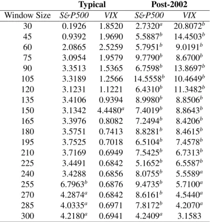
The test of Granger-causality is in table 1. The results shown that the indicator has a sensitivity problem for low values. However, for both returns and volatility it Granger-causes both the S&P500 and the VIX in the post-2002 context. For robustness sake, the analysis is replicated for subsamples of Post-2002: the crisis and the post-crisis (2007 to 2013) and an observation period (2003 to 2006). The results were similar, with the crisis period Granger-causing the S&P500 and the VIX for more windows than the observation period. An important observation is that, at 5% significance, just the window with 60 observations Granger-caused the S&P500 and the window with 30 observation Granger-caused the VIX index. This leads to an interpretation that, for the ICF, another indication of systemic crisis would be just after 2007.

1.3 Absorption Ratio

This indicator was developed by (KRITZMAN et al., 2011) and is based mainly on the eigenvalue decomposition of the covariance matrix (COV). The proposed indicator begins with:

(18)

Table 1 – Index Cohesion Force and Granger-Causation in the S&P500 and the VIX: in this table the values are the F-statistic of the Granger-causality tests. In the Typical period the results were much weaker for both the S&P500 and the VIX.

Typical Post-2002

Window Size S&P500 VIX S&P500 VIX

30 0.1926 1.8520 2.7320a _20.8072b

45 0.9392 1.9690 5.5887b _14.4503b

60 2.0865 2.5259 5.7951b _9.0191b

75 3.0954 1.9579 9.7790b _8.6700b

90 3.3513 1.5365 6.7598b _13.8697b

105 3.3189 1.2566 14.5558b _10.4649b

120 3.1231 1.1221 6.4310b _11.3482b

135 3.4106 0.9394 8.9980b _8.8506b

150 3.1342 4.4480a _7.4019b _8.8643b

165 3.3976 0.8082 7.2494b _8.4206b

180 3.5751 0.7413 8.8281b _8.4615b

195 3.7525 0.7018 6.5104b _7.4578b

210 3.7169 0.6949 7.5425b _6.7313b

225 3.4491 0.6842 5.1652b _6.5587b

240 3.4288 0.6856 8.0755b _5.5589a

255 6.7963b _0.6876 _9.4735b _5.7100a

270 4.2874a _0.6842 _8.6161b _4.5440a

285 4.0335a _0.6971 _7.8172b _4.2070a

300 4.2180a _0.6941 _4.2409a _3.1583 a_{significant at 5%;}b_{significant at 1%}

beingV the eigenvector matrix and Ψthe eigenvalue matrix. From the eigenvaluesψ,

the measure is built as:

AR=

∑n i λ

2

Ei ∑N

j λ2Aj

(1.5)

where σ2_E is the eigenvalue,σ2_A is the variance of an asset, N is the number of assets

and n is the number of eigenvalues used to calculate the index. (KRITZMAN et al.,

2011) recommends nto be approximately one fifth of N. Based on this, the indicator

(19)

the absorption ratio:

∆AR= (AR15 Day−AR1 Year)

σAR1 year

(1.6) This indicator Granger-caused the VIX for both periods (typical and post-2002) at 1%. Its impact on the S&P500 was significant at 5%.

1.4 Eigenvalue Entropy

The objective of this section is to discuss the mathematical properties of complexity measures based on entropies of eigenvalues.

1.4.1 The Indicator

Following (REZEK; ROBERTS, 1998) and (SABATINI, 2000) is possible to write a measure of entropy based on Singular Value Decomposition. This decomposition, for a positive semi-definite matrix, is the same as an EigenDecomposition. It means a correlation matrixΣ(nxn)can be decomposed as:

Σ =VΛVT (1.7)

where Λis the eigenvalue matrix and V is the eigenvector matrix. These eigenvalues

can be normalized using:

bλ= λ

tr(Σ) =

λ

n (1.8)

and a measure of entropy with the same functional form as Shannon Entropy(COVER; THOMAS, 2012; SHANNON, 1948):

−∑

i

pilogpi, (1.9)

is usually used. In this paper, a further analysis of those entropy based measures is provided. Based on Lewis (LEWIS, 1996) it can be seen that the derivative of a entropy with the functional form of Rényi Entropy (RÉNYI et al., 1961) is:

∂H(λ(X))

∂X =V

∂H(λ(X))

∂λ V

(20)

and

∂H(λ(X))

∂λi

= 1

1₋α αλα−1

i

∑n i=1λαi

(1.11) As long as correlation matrices X are positive semi-definite, this derivative is

non-positive for any possible eigenvalue and α _≥ 2. Therefore, the diagonal matrix Λ′,

composed by the derivatives of the entropy by its own eigenvalues, is negative semi-definite. We can observe that the signal of X elements is the opposite of the ones inX

and, internally, they are determined by the eigenvector matrix. As long asV is the same

matrix for both cases, the only case they have equal signals — the derivative matrix is all zero except by the diagonal — is when the correlation matrix is also zero in the non-principal diagonal elements: uncorrelated columns.

The function has the same functional form as Rényi entropy — a concave symmet-ric function — and, therefore, reaches its maximum when all normalized eigenvalues are equal: uncorrelated matrix. It reaches its minimum when just one eigenvalue can explain all data: data is perfectly correlated. In our example we will setα=2, assuring

a non-positive derivative for any eigenvalue and leading to the entropy:

H(X)= ₋log∑

i

bλ2_i (1.12)

Shannon Entropy is a limit case of Rényi entropy whenα_−→1. Taking the deriva-tives of Shannon Entropy, there are some characteristics that are different.

∂H(λ(X))

∂λi

= ₋(1₋logbλ) (1.13)

It is easy to see that if the largest eigenvalue is smaller than 1

e then the matrix is

positive-definite and, as Rényi Eigenvalue Entropy withα = 2, reaches a critical point

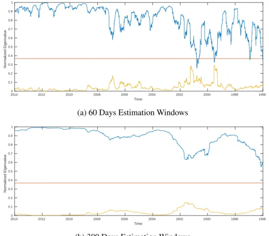
with the uncorrelated data. Otherwise, as usual with financial data, it is indefinite. Figure 1 exhibits how the two largest eigenvalues behave across time. With the win-dow estimation of correlations equal to 300, the derivatives matrix is always indefinite. However, this is not necessarily true for other windows. Using the window of 60 trad-ing days, for example, at some points the matrix was positive-definite. Related to the window size, it is remarkable that sometimes the second eigenvalue atW =60 is almost

(21)

Time

2014 2012 2010 2008 2006 2004 2002 2000 1998 1996

Normalized Eigenvalue 0 0.1 0.2 0.3 0.4 0.5 0.6 0.7 0.8 0.9 1

(a) 60 Days Estimation Windows

Time

2014 2012 2010 2008 2006 2004 2002 2000 1998 1996

Normalized Eigenvalue 0 0.1 0.2 0.3 0.4 0.5 0.6 0.7 0.8 0.9 1

(b) 300 Days Estimation Windows

Figure 1 – First and Second eigenvalues over time. The dividing line is set at 1

e. This

line is crossed for the 60 Days Estimation Window, but not for 300 Days.

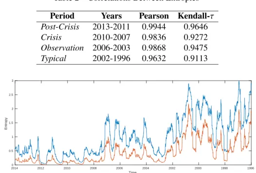
A question arises: how does Shannon Eigenvalue Entropy react to financial data? It is intuitive to believe it behaves concavely just as Rényi Eigenvalue Entropy because the Shannon Entropy is concave. A conclusive analysis is possible by comparing the derivatives matrix of Shannon Eigenvalue Entropy signs with the ones in correlation matrix. With the available data, all the signs were the same as the correlation: it means the Shannon Entropy acts with uncorrelated data as a local minimum. A confirmation can be drawn using its comparison with Rényi Eigenvalue Entropy. A correlation of 0.9760 between those entropies was drawn for the whole data. The correlation per periods using the sliding window of 60 days is in table 2.

We can see that the correlation is high for all periods. It is stable within the different

(22)

Table 2 – Correlations Between Entropies Period Years Pearson Kendall-τ

Post-Crisis 2013-2011 0.9944 0.9646 Crisis 2010-2007 0.9836 0.9272 Observation 2006-2003 0.9868 0.9475 Typical 2002-1996 0.9632 0.9113

Time

2014 2012 2010 2008 2006 2004 2002 2000 1998 1996

Entropy

0 0.5 1 1.5 2 2.5 3

Figure 2 – The orange line is Shannon Eigenvalue Entropy and the blue line is Rényi Eigenvalue Entropy. The indicators were calculated using a 60 days window.

level of the largest eigenvalue (KENETT et al., 2011), higher in the typical period. It is safe to that say the entropies behave similarly.

1.4.2 Stock Market Indexes and Entropy

A first conclusion taught in text books of modern portfolio theory (MARKOWITZ, 1952) is “diversification is good because it eliminates idiosyncratic risk”. However, taking the two assets case as an example, it is possible to perceive how correlations af-fects how things can be diversified. In the limit case whereρ= ₋1 it is possible to have

a riskless portfolio, but for anyρ >₋1, this is impossible. The higher theρ, the higher the minimum risk. Moreover, in econophysics, correlation networks (MANTEGNA; STANLEY, 1999) are a very important tool — the second level of complexity, in the definition of (BONANNO; LILLO; MANTEGNA, 2001) — that must be preserved as long as it is possible.

(23)

re-Chapter 1. Volatility and Correlation-Based Systemic Risk Measures in the US Market 22

spects:

∂H(Σ)

∂ρi j

> 0 or ∂H(Σ) ∂ρi j

<0, _∀ρi j ∈(−1,1) (1.14)

It is easy to see that both Shannon and Rényi Eigenvalue Entropies do not respect this characteristic. They have a global maximum with uncorrelated data. The measure we want must have corner solutions, growing or decreasing monotonically. This is not possible using a measure based on eigenvalues as proven by the following proposition. Proposition 1. There is not any symmetric spectral function that allows a representation that is monotonically increasing with any correlation.

Proof. We begin considering the function:

f(Λ)=

n

∑

i=1

λi =tr(X) (1.15)

which is the summation of the eigenvectors of the correlation matrixX. Diff

erentiat-ing this equation by an arbitrary correlation and considererentiat-ing the trace of the correlation matrix constant:

n

∑

k=1

∂λk(X)

∂ρi j

=0 (1.16)

Therefore:

∂λn

∂ρi j

= ₋

n−1

∑

k=1 ∂λk

∂ρi j

(1.17) We setλnto be an eigenvalue affected by the variation on a correlation matrix

ele-ment. If anyλis not affected by the correlation variation, then the eigenvalues are not

injective because they will assume the same value for different correlations; therefore

g(λ) cannot be injective; it does not allow a representation of assets correlations.

There are two possible scenarios: either the derivative ofλnto correlation is positive

(24)

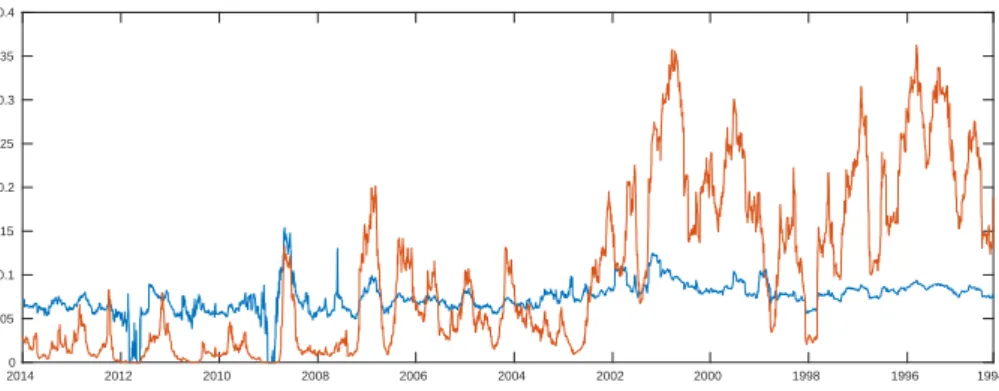
Figure 3 – The proportion of negative correlations is the orange line and the largest eigenvalue is the blue line.

Time

2014 2012 2010 2008 2006 2004 2002 2000 1998 1996 1994

Size

0 0.1 0.2 0.3 0.4 0.5 0.6 0.7 0.8 0.9 1

Figure 4 – The proportion of negative correlations is the orange line and the second eigenvalue is the blue line.

Time

2014 2012 2010 2008 2006 2004 2002 2000 1998 1996

Size

0 0.05 0.1 0.15 0.2 0.25 0.3 0.35 0.4

a solution to the characteristic polynomial composed by functions of the correlations —, there are some values on which the negative change in correlation generates a similar outcome in terms of eigenvalues: it is a permutation of a positive change. A symmetric function is invariant to permutations matrix by definition, therefore it is not possible to

define this function. _□

(25)

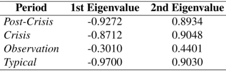
Table 3 – Correlations Between Presence of Negative Correlations and Eigenvalues Period 1st Eigenvalue 2nd Eigenvalue

Post-Crisis -0.9272 0.8934 Crisis -0.8712 0.9048 Observation -0.3010 0.4401 Typical -0.9700 0.9030

Results have shown high correlations for all periods, except by the observation – set to be from 2003 to 2006 – which had the absolute value of correlation below 0.5. However, it is not necessarily true for other windows. Considering the window of 60 trading days, the lowest correlation is the second eigenvalue with 0.6483, with all others larger than 0.7.

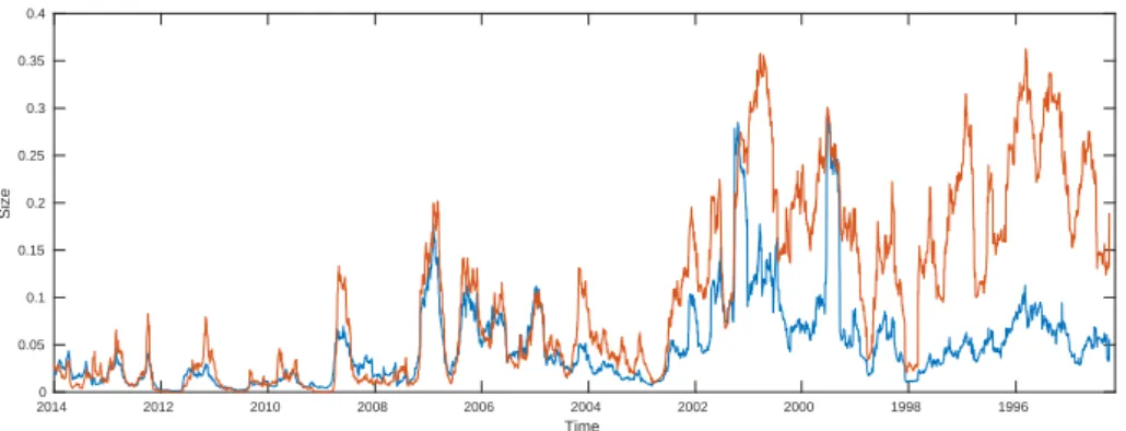
In order to analyse the impact of these negative correlations, it is important to know the size of the negative correlations. In figure 5 we can see that, although the mean negative correlation is correlated with the proportion of negative correlations, its level is usually below 0.15. This level, compared to the mean positive correlation, is very low. Another test is made using a linear regression of eigenvalue entropy by the mean correlation and the mean negative correlation. This leads to an analysis of how much the negative correlation affects the eigenvalue and the direction of this effect. Two

re-gression models are used. The equations are:

EEt =β0+β1∗Mean Correlation (1.18)

EEt =β0+β1∗Mean Correlation+β2∗Mean Negative Correlation (1.19)

Considering the estimation window of 60 days, the betas and theR2 are in table 4.

It is possible to perceive that, if the mean negative correlations is higher, the entropy gets lower. The same applies to mean correlation — that is just the effect of positive

(26)

2014 2012 2010 2008 2006 2004 2002 2000 1998 1996 1994 0

0.05 0.1 0.15 0.2 0.25 0.3 0.35 0.4

(a) Relation of the proportion of negative correlations and the mean negative correlation. It is possible to see that the series are correlated.

2014 2012 2010 2008 2006 2004 2002 2000 1998 1996 1994 0

0.1 0.2 0.3 0.4 0.5 0.6 0.7 0.8

(b) Series of the mean negative correlation and the mean positive correlation. It is possible to see that the impact of the negative correlations is smaller than the impact of positive correlations.

Figure 5 – Images showing the patterns of positive and negative correlations.

(27)

Table 4 – Results for regressions. Model 1 is better explained in equation 18 and model 2 is represented in equation 19. The estimates show that higher mean positive correlation leads to a smaller entropy, as well higher mean negative correla-tion leads to the same result. This confirms the theoretical prediccorrela-tion about eigenvalue entropies being non-representative of “correlation risk”.

Full Sample Post-2002 Typical

Model 1 Model 2 Model 1 Model 2 Model 1 Model 2

β0 2.4719 1.3409 1.6081 1.2354 3.1148 2.4369

β1 -4.9472 -2.4174 -2.7862 -2.0642 -8.1509 -6.1939

β2 - 54.2561 - 42.4107 - 28.8506

1.4.3 Granger Causality of Returns and Volatility

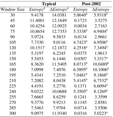
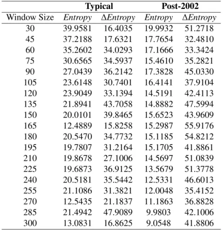
Although Eigenvalue Entropy does not have some desirable mathematical properties, it was shown that it Granger-causes (GRANGER, 1969) index returns (CARAIANI, 2014). Table 5 collects some results of estimative of Eigenvalue Entropy — in this section, it refers exclusively to Shannon Eigenvalue Entropy — as Granger-causing the S&P500 returns. The tests were also built for the ∆Entropy indicator (CARAIANI,

2014):

∆Entropy_t =Entropy_t₋Entropy_t₋₁ (1.20)

It is clear that from 1997 to 2002 the Eigenvalue Entropy Granger-caused the S&P500 Returns at 1%, as well its Delta for all windows. However, this predictive power is weaker in the post-2003 period. There is not any clear pattern for when the Eigenvalue Entropy or its delta will Granger-cause when we change the estimation window.

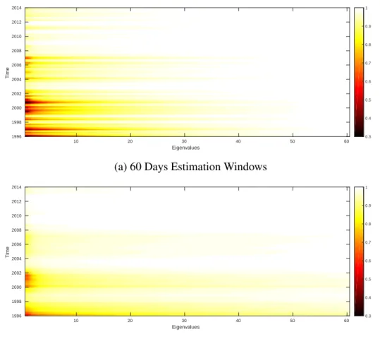
The period Eigenvalue Entropy predicts better the S&P500 is coherent with more eigenvalues being necessary to explain the data before 2003. This is shown at figure 6a and figure 6b, heat maps that show how much the eigenvalues explain the data. Figure 6a is the heat map withW =60 and figure 6b is the one withW = 300.

It is seen that, even though there are some differences between the images, the

typ-ical period has lower cumulative eigenvalues. At this period, there are more negative correlations, as illustrated by images 3 and 4. This would affect the behaviour of the

(28)

win-Chapter 1. Volatility and Correlation-Based Systemic Risk Measures in the US Market 27

dow of 300 Granger-causes the S&P500 and have higher first eigenvalue; the estimation using 60 observations did not, but have a smaller first eigenvalue.

A possible economic explanation for this behaviour is that the systemic risk in fact is higher after 2002. In qualitative terms, after 2008 the eigenvalue entropy is almost always below 1, leading to small effects in the returns. A simple robustness test is made

by selecting a window in the post-2002 sample where the mean eigenvalue entropy is higher than 1 — from April 1st, 2003 to January 8th, 2007 — to using a non-significant time horizon to build the indicator: 60 days. The result reinforced our hypothesis: The entropy was significant at 5% and its delta was significant at 1%.

Table 5 – Entropy, Returns and Granger-causality: in this table the values are the F-statistic of the Granger-causality tests. There is no clear pattern in how the window size affects the Granger-causation.

Typical Post-2002

Window Size Entropyb ∆Entropyb Entropy ∆Entropy

30 9.4178 14.0381 5.0640b _5.9318b

45 11.4001 12.1649 0.1723 3.5275 60 10.4254 12.0925 0.0034 2.7163 75 10.8654 12.7353 5.3338b _6.9404b

90 5.9724 9.5833 0.0134 2.9661 105 7.7330 9.0116 4.7423b _6.9506b

120 10.1517 12.1872 4.2518a _7.3494b

135 5.3197 6.2245 0.0375 1.9613 150 5.5453 6.1446 0.0307 3.3317a

165 8.3620 11.5405 8.0713b _10.0489b

180 7.0998 7.4076 6.5895b _10.1006b

195 5.4341 7.2510 7.0481b _9.1868b

210 7.2082 8.0438 5.4145b _6.7532b

225 4.4191 5.2776 0.1371 6.6094b

240 9.0322 10.0688 5.3505b _8.1269b

255 7.6665 8.6259 0.1241 3.3599 270 9.3776 9.9213 0.1145 2.8581 285 7.5463 7.9704 0.0714 3.5506 300 9.0975 11.9340 0.0316 5.0223a

(29)

Eigenvalues

10 20 30 40 50 60

Time 2014 2012 2010 2008 2006 2004 2002 2000 1998 1996 0.3 0.4 0.5 0.6 0.7 0.8 0.9 1

(a) 60 Days Estimation Windows

Eigenvalues

10 20 30 40 50 60

Time 2014 2012 2010 2008 2006 2004 2002 2000 1998 1996 0.3 0.4 0.5 0.6 0.7 0.8 0.9 1

(b) 300 Days Estimation Windows

Figure 6 – Heat Maps of Eigenvalue cumulative values. In the 300 days estimation win-dows the concentration of risk in the first eigenvalues is stronger.

The same test is done using the VIX index. This index is calculated using the im-plicit volatility of the S&P500 options. This is more coherent with the argument that Eigenvalue Entropy is a systemic risk measure (KENETT et al., 2011). The results are in table 6.

(30)

Table 6 – Entropy, Volatility and Granger-Causation: in this table the values are the F-statistic of the Granger-causality tests.

Typical Post-2002

Window Size Entropy ∆Entropy Entropy ∆Entropy

30 39.9581 16.4035 19.9932 51.2718 45 37.2188 17.6321 17.7654 32.4810 60 35.2602 34.0293 17.1666 33.3424 75 30.6565 34.5937 15.4610 35.2821 90 27.0439 36.2142 17.3828 45.0330 105 23.6148 30.7401 16.4141 37.9104 120 23.9049 33.1394 14.5191 42.4113 135 21.8941 43.7058 14.8882 47.5994 150 20.0101 39.8465 15.6523 43.9609 165 12.4889 15.8258 15.2987 55.9176 180 20.5470 34.7732 15.1185 54.8212 195 19.7807 31.2164 15.1705 41.8861 210 19.8678 27.1006 14.5697 51.0839 225 19.6873 36.9125 13.5679 51.3778 240 20.5181 35.5442 12.5331 46.6013 255 21.1086 31.3821 12.0048 35.4152 270 12.5435 21.1837 11.1863 36.8828 285 21.4942 47.9089 9.9803 42.1006 300 13.0831 16.8625 9.0548 41.8806

All indicators are significant at 1%

1.5 Discussion

There are some remarkable differences between the indicators. It is possible to see

that the Granger-causation power of the ICF is higher post-2002, being usually non-significant in the Typical window. The result for the eigenvalue entropy is different:

significant for the VIX in both windows and for returns before 2002, not significant for returns after 2002.

(31)

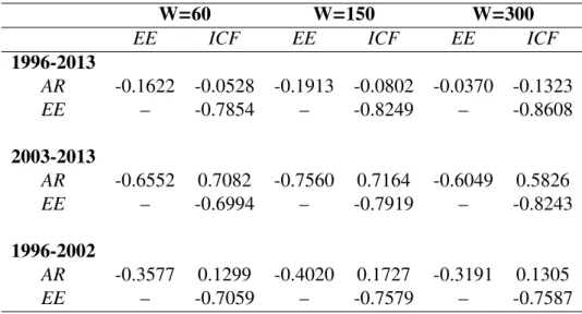
Table 7 – Correlations between indicators. There are subsamples analysis, using the division between typical and post-2002 periods. In this table, AR is the ab-sorption ration and EE is the Eigenvalue Entropy.

W₌60 W₌150 W₌300

EE ICF EE ICF EE ICF

1996-2013

AR -0.1622 -0.0528 -0.1913 -0.0802 -0.0370 -0.1323

EE – -0.7854 – -0.8249 – -0.8608

2003-2013

AR -0.6552 0.7082 -0.7560 0.7164 -0.6049 0.5826

EE – -0.6994 – -0.7919 – -0.8243

1996-2002

AR -0.3577 0.1299 -0.4020 0.1727 -0.3191 0.1305

EE – -0.7059 – -0.7579 – -0.7587

considering all periods, the correlation is weak between Absorption Ratio and the other indicators.

A deeper question is how the underlying techniques used to analyse the correlations matrices are representative of the behaviour of the correlations. Two analysis are built for understand this behaviour: one simply assessing the correlation between eigenvalue entropy and mean correlation in different windows — Typical and Post-2002 time

win-dows — and the other capturing differences in positive returns and negative returns. The

results are in table 8 and 9. As we can see, the relationship is negative and very strong for all windows — revealing that, besides the distortion caused by negative correlations, the eigenvalue entropy is a good measure of the correlations —, without great diff

er-ences between them. The behaviour is constant even for positive and negative periods of markets. This relation is slightly larger than the simpler relation between the mean correlation and the first eigenvalue, as shown at table 10.

1.6 Conclusion

(32)

corre-Chapter 1. Volatility and Correlation-Based Systemic Risk Measures in the US Market 31

Table 8 – Results for mean correlation and eigenvalue entropy in different periods.

Pearson Kendall

Window Size Typical Post-2002 Typical Post-2002

60 -0.9385 -0.8838 -0.9334 -0.9416 150 -0.9270 -0.9090 -0.9468 -0.9078 300 -0.9400 -0.9399 -0.9163 -0.9045

Table 9 – Results for mean correlation and eigenvalue entropy when the mean return is positive or negative.

Pearson Kendall

Window Size Positive Negative Positive Negative

60 -0.9175 -0.8821 -0.9577 -0.9534 150 -0.8747 -0.8800 -0.9463 -0.9277 300 -0.8717 -0.9088 -0.9485 -0.9421

Table 10 – Results for mean correlation and largest eigenvalue in different periods.

Pearson Kendall

Window Size Typical Post-2002 Typical Post-2002

60 -0.8326 -0.9049 -0.9042 -0.8999 150 -0.8677 -0.8951 -0.8623 -0.8675 300 -0.9091 -0.8900 -0.8636 -0.7709

lations and failed to Granger-cause both returns and implied volatility of the American market in the windows with typical behaviour. In times of high systemic risk, how-ever, the indicator was useful to understand the behaviour of the S&P500 and the VIX indices, besides the failure in typical periods.

The Absorption Ratio is briefly discussed and it Granger-causes the VIX index for all periods considered. Its effect on the S&P500 is significant; it is the only indicator

considered here that Granger-caused returns. This index is strongly correlated to the ICF in the Post-2002 window. In the other windows, this effect is weaker.

Finally, eigenvalue entropy is deeply studied in this paper. Its origins in biology do not imply in being a bad indicator for finance. In the theoretical front the eigenvalue entropy has difficulties to represent correlations — with an empirical confirmation of

(33)

indica-Chapter 1. Volatility and Correlation-Based Systemic Risk Measures in the US Market 32

tor is highly correlated to the mean correlation, dismissing some preoccupations about its behaviour. The eigenvalue entropy is negatively correlated to the ICF and to the Absorption Ratio.

These analysis revealed that there are some measurement insensitivities in the sys-temic risk indicators based on correlation matrices. However, dealing with the VIX index, both Absorption Ratio and the Eigenvalue Entropy were able to Granger-cause implied volatilities. The Index Cohesion Force did not Granger-caused any systemic crisis before 2007.

However, for eigenvalues entropies was previously stated that they would Granger-cause returns. This affirmation is dismissed depending on the window and period

(34)

33

2 Correlation-Based

Systemic

Risk

Measures

and

Stock

Market

Regimes

2.1 Introduction

A financial crisis may be troublesome for everyone in society. The economic panorama after in the post-2008 subprime crisis is not bright as may be exemplified by the Eurocri-sis (REIS, 2013; FABBRINI, 2013; STOCKHAMMER; ONARAN, 2012), huge gov-ernmental debt (REINHART; ROGOFF, 2011) and political radicalism (CASTELLS, 2013). If there is a place that seems very calm, surprisingly, that is the US stock mar-ket. In figure 1, it is possible to see that the S&P500 index is growing in an apparently sustained way since the bottom of the crisis in 2008.

This paper uses a simple systemic risk measures to assess what is happening in the US stock market: the absorption ratio by (KRITZMAN et al., 2011). Previous literature — the first paper of this dissertation — shows this measure Granger-causing the VIX index, but they do not have a strongly significant impact (p-value>0.01) in returns after

2002. The interpretation proposed here is to understand the Absorption Ratio and the Herfindahl-Hirschman Index as a concentration measure of the risk factors estimated using the principal component analysis and understand how does it affects the stock

market behaviour.

Absorption Ratio is a well-known measure discussed in the survey by (BISIAS et al., 2012). Its main idea is to use the concentration of risk in the largest eigenvalues of a given portfolio to assess the systemic risk. It is built using the covariance matrix. This indicator was also used for funds returns by (BILLIO et al., 2012) The eigenvalue entropy was applied in the econophysics literature (CARAIANI, 2014; KENETT et al., 2011) using correlation of assets. They are examples of what can be considered correlation-based systemic risk indicators.

(35)

indi-Chapter 2. Correlation-Based Systemic Risk Measures and Stock Market Regimes 34

Figure 7 – The S&P500 over time.

cators. There are measures based in macroeconomic analysis directly (BORIO; LOWE, 2004; BORIO; DREHMANN, 2009). These indicators are responsible for understand if the macroeconomic condition is prone to systemic collapses. (ALESSI; DETKEN, 2011) concluded that credit and monetary contractions are the most useful series to analyse the financial environment. It is possible to figure that the objective of these indicators is different from a simple risk concentration/dispersion tool.

A more similar tool are based in network effects (GLASSERMAN; YOUNG, 2015;

ACEMOGLU; OZDAGLAR; TAHBAZ-SALEHI, 2015). These measures are related to contagion risk and how much a node of a network can impact in other nodes. For instance, (BILLIO et al., 2012) created a network of Granger-causation between returns of hedge funds, brokers, insurance companies and banks. Other approaches are based in network econometrics (DIEBOLD; YILMAZ, 2014). (BARIGOZZI; BROWNLEES, 2014) developed an algorithm based in the LASSO estimator that considers both con-temporary and long run correlations.

(36)

Chapter 2. Correlation-Based Systemic Risk Measures and Stock Market Regimes 35

random matrix theory (LALOUX et al., 2000; JUNIOR; FRANCA, 2012) are used to detect abnormal patterns in the eigenvalues derived from correlations. The usage of this technique applied to Absorption Ratio is developed in this paper and a novel indicator, the filtered Absorption Ratio (fAR) is built. A random matrix theory application is used to check how the eigenvalues used in the correlation matrix are different from the whole

set of eigenvalues of financial data. This analysis leads to the conclusion of overesti-mation of risk factors in traditional Absorption Ratio indicator. While (KRITZMAN et al., 2011) recommends 70 eigenvalues for the dataset used here, an indicator using 15 filtered eigenvalues is built in this application.

The procedure of filtering eigenvalues is to simply use a historical volatility model to fit the returns before estimating the covariance matrix. The residuals are bootstrapped to generate new random covariance matrices. The reasons for this procedure are related to the literature on Value-at-Risk, especially (BARONE-ADESI; GIANNOPOULOS; VOSPER, ; BARONE-ADESI; GIANNOPOULOS; VOSPER, 2002), and are best de-scribed in section 3. The traditional indicators are presented in section 2.

A more complex analysis is built using the Markov Switching method proposed by (PEREZ-QUIROS; TIMMERMANN, 2000; DING, 2012). The returns are analysed using a time-varying transition probability matrix, being the probabilities function of the indicators. Implementations using two and three states are built and the model that better fits the data is the filtered Herfindahl-Hirschman with 3 states.

Qualitatively, the behaviour of the indicator is not very different from the model

with fixed transition probabilities. However, a more deep backtesting shows that adding a systemic risk model to the transition probabilities leads to a more stable prediction of bad economic moments. This test was built with the filtered Absorption Ratio to show that adding a model — even one that has ambiguous results (using AIC and BIC) compared to the time-fixed transition probabilities — can lead to a better prediction. This analysis is developed in section 4.

2.2 Principal Components and Risk Factors

(37)

Index (HHI) (RHOADES, 1993; CETORELLI, 1999). In finance, (KRITZMAN et al., 2011) discusses some recent measures are analogous to them.

The Absorption Ratio is built using the eigenvalues from the covariance matrix and the Eigenvalue Entropies are built using correlation matrices. In the first paper of this dissertation, was shown that the Shannon Eigenvalue Entropy has similar properties of Rényi Eigenvalue Entropy, that is an immediate transformation of the HHI index. In this paper, the measure considered is the Absorption Ratio and its HHI considered in (KRITZMAN et al., 2011).

The measures may be constructed with normalized eigenvalues:

ˆ λ= λ

tr(Σ) =

λ

N (2.1)

whereNis the number of assets analysed,λis an eigenvalue andΣis the matrix analysed

— covariance for absorption ratio and correlation for eigenvalue entropy. The formula for absorption ratio is simply:

AR=

N/5

∑ ˆ

λi (2.2)

whereN is the number of assets used to calculate the index. Another indicator

sug-gested is the standardized shift in the absorption ratio, constructed using the difference

between the short term and the long term averages of the Absorption Ratio:

ARshi f t =

(AR15 Days −AR1 Year)

σAR1 year

(2.3) The Herfindahl-Hirschman index of the eigenvalues may be written as:

HHI =

N

∑ ˆ

λ2_i (2.4)

This index was tested — when calculated using the covariance matrix estimated with 500 trading days — in (KRITZMAN et al., 2011). This indicator was shown to perform worst than the Absorption Ratio.

The last indicator is a hybrid between theARshi f t and the HHI. It is simply:

HHIshi f t =

(HHI15 Days−HHI1 Year)

σHHI1 year

(38)

2.3 Filtered Concentration

A novel systemic risk indicator based in the Random Matrix Theory is proposed in this section. Random Matrix Theory is based in the distribution of eigenvalues of a random matrix with normal observations. If the dimension of the analysed random matrix is

TxNandT,N _{→ ∞}, whereQ= _NT is greater than one and is finite, then this distribution,

also know as Marcenku-Pastur is:

ρ(λ)= Q

2πσ2

√

λmax−λ

√

λ₋λmin

λ

λmax

min = σ

2₍₁

±

√₁

Q)

(2.6)

This distribution provides a theoretical framework to work with, but as it is possible to see, Q is not designed to the approach using covariances directly and it is based in

normal distributions. In order to overcome these issues, a quasi-Monte Carlo simulation of the stock returns is used. For each stock series an AR(1)+GARCH(1,1)

(BOLLER-SLEV, 1986) is estimated and the parameters and residuals are stored. They are used to generate new series by bootstraping the residuals, in a process inspired in the Fil-tered Historical Simulation of Value-at-Risk (BARONE-ADESI; GIANNOPOULOS; VOSPER, ; BARONE-ADESI; GIANNOPOULOS; VOSPER, 2002). The reason for adopting this process is to filter the individual and predictable risk from the systemic risk analysis. These new series are used to create 10.000 new matrices 500x346 and calculate an empirical distribution of eigenvalues.

The data used in this paper was taken from Yahoo! Finance and its composed by all stock prices — 346 firms — from the S&P500 (collected August 31st 2014) from 1994 to 2013 available without missing observations. After calculating theARshi f t, this data is

from 1996 to 2013. The estimated Random Matrix Theory parameters areλcov

min= 0.0244

andλcov

max=3.5637.

These parameters are used for estimating the optimalnfor the traditional Absorption

Ratio (tAR) and for checking if the majority of them are really useful compared to the eigenvalues eliminated. This is exhibited in figure 2. This figure shows the optimaln

using theλcov_estimated.

(39)

Figure 8 – The number of non-noisy eigenvalues over time, using as criterionλit< λcovmax.

0 500 1000 1500 2000 2500 3000 3500 4000 0

5 10 15

Figure 9 – The blue line is the value of tAR, the red line is the value of fAR, the yellow line is the value of the HHI and the purple line is the value of filtered HHI.

0 500 1000 1500 2000 2500 3000 3500 4000 -2.5

-2 -1.5 -1 -0.5 0 0.5 1 1.5 2 2.5

Absorption is excessive. The procedure usingn _≈ N/5 may, therefore, add some noise

to the estimative. However, to avoid jumps by accepting a different number of

eigen-values — and considering that there is some estimation error inλcov

max — in fAR there

is a fixed number of 15 eigenvalues. Figure 3 shows how the filtered Absorption Ratio (fAR) captures a different behaviour than tAR.

Two simple metrics are useful to compare if the impact of noisy eigenvalues in the Absorption Ratio is smaller than in the HHI. The metric for the Absorption Ratio is:

NAR =

∑n i>aλi

∑n i=1λi

(40)

Figure 10 – The blue line is the distortion of tAR, the red line is the distortion of HHI, the yellow line is the value for fAR and the purple line is the value of filtered HHI. It is clear that the Absorption Ratios have more noise than Herfindahl-Hirschman Indexes

0 500 1000 1500 2000 2500 3000 3500 4000 4500 5000 0.3

0.4 0.5 0.6 0.7 0.8 0.9 1

The metric for noise in the HHI is analogous and defined as:

NHHI =

∑N i>aλˆ2i

∑N i=1λˆ

2

i

, λa > λmax (2.8)

These metrics can be used for any kind of eigenvalue estimation, as the ones based in covariances and the ones based in correlations. The comparison of the two metrics allows to verify how much the eigenvalues that survived the RMT analysis influence the whole behaviour of the indicator. Their comparison forλin figure 4 shows the impact of noisy eigenvalues is smaller in the Henfindahl-Hirschman Index than in the Absorption Ratio.

2.4 Systemic Risk Impact on Returns

(41)

measures. They were estimated using the MATLAB toolbox developed by (PERLIN, 2012). The estimation method is described in (DING, 2012).

The model is composed by a simple regression of:

yt =αS +εt;ε∼ N(0, σS t) (2.9)

The parameters are regime-dependent (S). The regime follows a Markov Chain with

transition probability:

 

₁₋q11_q₁₁ ₁₋q12_q₁₂  

, (2.10)

for models with two states and 

  

q11 q12 q13

(1₋q11)q21 (1−q12)q22 (1−q13)q23

(1₋q11)(1−q21) (1−q12)(1−q22) (1−q13)(1−q23)

  

 (2.11) for models with three states. qi j is built by a cumulative normal distribution of the

parameters estimated.

Five models were tested: the Markov Switching with fixed transition probabilities, the time-varying transitions probability with shifts of the Absorption Ratio and the fil-tered Absorption Ratio, the traditional HHI and the filfil-tered HHI. The initial estimation is using two regimes. Qualitatively, there is not any great difference in the behaviour of

(42)

Null tAR fAR tHHI fHHI

Mean(1) 0.00068∗∗ _0.00072∗∗ _0.00070∗∗ _0.00069∗∗ _0.00068∗∗

Mean(2) -0.00102▲ -0.00102▲ -0.00094 -0.00102▲ -0.00099▲

Variance(1) 0.00007∗∗ 0.00007∗∗ 0.00007∗∗ 0.00007∗∗ 0.00007∗∗ Variance(2) 0.00042∗∗ 0.00041∗∗ 0.00040∗∗ 0.00042∗∗ 0.00042∗∗

q(1,1)

intercept 2.38702∗∗ _2.30245∗∗ _2.43136∗∗ _2.36852∗∗ _2.41771∗∗

slope -1.26944∗∗ _-1.72267∗∗ _-0.53695∗∗ _-0.91671∗∗

q(1,2)

intercept -2.015817∗∗ _-1.84660∗∗ _-1.87463∗∗ _-1.93864∗∗ _-1.90950∗∗

slope 0.17833 0.28477 -0.13967 -0.32806

(43)

Figure 11 – The smoothed probabilities of each stage. The left upper graph is the model with fixed transition probabilities, the left down is the model with fAR, the right upper is the model with tAR and the right down is the model with fHHI.

0 500 1000 1500 2000 2500 3000 3500 4000 0 0.2 0.4 0.6 0.8 1

Figure 12 – The smoothed probabilities of each stage. The left upper graph is the model with fixed transition probabilities, the left down is the model with fAR, the right upper is the model with tAR and the right down is the model with fHHI.

0 500 1000 1500 2000 2500 3000 3500 4000 0 0.2 0.4 0.6 0.8 1

(44)

Null tAR fAR tHHI fHHI

Mean(1) 0.00103 0.00105 0.00105 0.00105 0.00104 Mean(2) 0.00000 -0.00002 0.00000 0.00000 0.00000 Mean(3) -0.00145 -0.00144 -0.00145 -0.00140 -0.00145

Variance(1) 0.00003 0.00004 0.00004 0.00004 0.00004 Variance(2) 0.00013 0.00013 0.00013 0.00013 0.00013 Variance(3) 0.00072 0.00072 0.00072 0.00072 0.00072

q(1,1)

intercept 2.01298 1.92230 1.93812 1.96242 1.96373

slope -0.81559 -0.82155 -0.12265 -0.28364

q(1,2)

intercept -2.17118 -2.08696 -2.01077 -2.11983 -2.10034

slope -0.78979 -2.10906 -1.36293 -1.56122

q(2,2)

intercept 2.46963 2.55011 2.53419 2.53276 2.51523

slope -0.64459 -0.44246 -0.68893 -0.37534

q(2,3)

intercept -1.88472 -1.71002 -1.56399 -1.54774 -1.57997

slope -0.68925 -1.81345 -1.73296 -2.01499

(45)

2.5 Conclusion

In this paper the Absorption Ratio and the Herfindahl-Hirschman Index of Principal Components are analysed as tools for systemic risk management. The first conclusion is that, in the actual form, Absorption Ratio considers too many eigenvalues. The number fell from 70 to 15 in our dataset. The second conclusion is that using an indicator that considers the GARCH effects and the real distribution from data generates richer

dynamics.

The new indicators, the filtered Absorption Ratio and the filtered Herfindahl-Hirschman Index, were used in a Markov Switching with time-varying transition probabilities model. The model with both lower Akaike Information Criterion and lower Bayesian Informa-tion Criterion was the filtered Herfindahl-Hirschman Index with three regimes.

The usage of GARCH models to filter predictable shocks and the criteria from Ran-dom Matrix Theory are useful to select the principal components for the models. It is important to notice that Random Matrix Theory presents a simple way to select the number of components to financial applications and that correlation-based systemic risk factors may be condensed by its usage. The usefulness of this approach is clear in the Markov Switching tests proposed here.

(46)

45

Conclusion

As a final remark of this dissertation, an important point is to talk about black swans (TALEB, 2007; SORNETTE, 2009). The papers presented here show that the indicators discussed may be useful for detecting crises. Through the Markov Switching model, it was possible to predict reasonably the crisis period. Is it safe to say that systemic collapses can be foreseen now?

The right answer is that, if the causes are similar, then a new tool for predicting it is available. However, History is not tired of showing us how wrong we can be. The causes of the crisis may be different, as an unexpected default from a big country. How

will the indicators will work in this case? More studies are necessary to answer this question.

A truly forward looking systemic risk measure is hard to imagine, but it is necessary to achieve financial stability. Besides this measure does not exists by now, another tool, as the filtered Absorption Ratio, for observing some kinds of risk is useful. The main objective of this construct is to analyse past crises and see that similar causes may lead to a different outcome, as long as it is known that an ongoing instability is growing.

However, just creating new instruments is not sufficient. Analysing them deeply is

an important part of the process that, as seen in the papers, is not always considered. The indicators discussed had flaws and possible optimizations. One of the objectives of this dissertation was to develop the indicators to, finally, try to figure out how safe one can be using them.

Therefore, the main conclusion is that, despite not being fully protected, new simple instruments for understanding the financial environment are being built and, indeed, they are useful. They are quite accessible to any investor that is interested in building them. Nevertheless, another limitation of this dissertation is to not discuss how any additional common-knowledge about systemic risk may affect the market. For instance,

(47)

46

Bibliography

ACEMOGLU, D.; OZDAGLAR, A.; TAHBAZ-SALEHI, A. Systemic risk and stability in financial networks.American Economic Review, v. 105, n. 2, p. 564–608,

2015.

ALESSI, L.; DETKEN, C. Quasi real time early warning indicators for costly asset price boom/bust cycles: A role for global liquidity.European Journal of Political Economy, Elsevier, v. 27, n. 3, p. 520–533, 2011.

ALLEN, F.; GALE, D. Financial contagion.Journal of political economy, JSTOR,

v. 108, n. 1, p. 1–33, 2000.

BARIGOZZI, M.; BROWNLEES, C. T. Nets: network estimation for time series.

Available at SSRN 2249909, 2014.

BARONE-ADESI, G.; GIANNOPOULOS, K.; VOSPER, L. Var without correlations for nonlinear portfolios.Journal of Future Markets.

BARONE-ADESI, G.; GIANNOPOULOS, K.; VOSPER, L. Backtesting derivative portfolios with filtered historical simulation (fhs).European Financial Management,

Wiley Online Library, v. 8, n. 1, p. 31–58, 2002.

BILLIO, M. et al. Econometric measures of connectedness and systemic risk in the finance and insurance sectors.Journal of Financial Economics, Elsevier, v. 104, n. 3, p.

535–559, 2012.

BISIAS, D. et al. A survey of systemic risk analytics.US Department of Treasury, Office of Financial Research, n. 0001, 2012.

BOLLERSLEV, T. Generalized autoregressive conditional heteroskedasticity.Journal of econometrics, Elsevier, v. 31, n. 3, p. 307–327, 1986.

BONANNO, G.; LILLO, F.; MANTEGNA, R. N. Levels of complexity in financial markets.Physica A: Statistical Mechanics and its Applications, Elsevier, v. 299, n. 1,

p. 16–27, 2001.

BORIO, C. E.; DREHMANN, M. Assessing the risk of banking crises revisited.BIS Quarterly Review, 2009.

(48)

Bibliography 47

CAPUANO, C. The option-ipod: The probability of default implied by option prices based on entropy.IMF Working Papers, p. 1–29, 2008.

CARAIANI, P. The predictive power of singular value decomposition entropy for stock market dynamics. Physica A: Statistical Mechanics and its Applications, Elsevier,

v. 393, p. 571–578, 2014.

CASTELLS, M.Networks of outrage and hope: Social movements in the Internet age.

[S.l.]: John Wiley & Sons, 2013.

CETORELLI, N. Competitive analysis in banking: appraisal of the methodologies.

ECONOMIC PERSPECTIVES-FEDERAL RESERVE BANK OF CHICAGO, THE

FEDERAL RESERVE BANK OF CHICAGO, v. 23, p. 2–15, 1999.

COVER, T. M.; THOMAS, J. A.Elements of information theory. [S.l.]: John Wiley &

Sons, 2012.

DIEBOLD, F. X.; YILMAZ, K. On the network topology of variance decompositions: Measuring the connectedness of financial firms.Journal of Econometrics, Elsevier,

v. 182, n. 1, p. 119–134, 2014.

DING, Z. An implementation of markov regime switching model with time varying transition probabilities in matlab.Available at SSRN 2083332, 2012.

DUFFIE, D.; PAN, J. An overview of value at risk.The Journal of derivatives,

Institutional Investor Journals, v. 4, n. 3, p. 7–49, 1997.

ENGLE, R. Dynamic conditional correlation: A simple class of multivariate

generalized autoregressive conditional heteroskedasticity models.Journal of Business

&Economic Statistics, Taylor & Francis, v. 20, n. 3, p. 339–350, 2002.

FABBRINI, S. Intergovernmentalism and its limits assessing the european union’s answer to the euro crisis. Comparative Political Studies, SAGE Publications, p.

0010414013489502, 2013.

GLASSERMAN, P.; YOUNG, H. P. How likely is contagion in financial networks?

Journal of Banking&Finance, Elsevier, v. 50, p. 383–399, 2015.

GRANGER, C. W. Investigating causal relations by econometric models and

cross-spectral methods.Econometrica: Journal of the Econometric Society, JSTOR, p.

424–438, 1969.

JUNIOR, L. S.; FRANCA, I. D. P. Correlation of financial markets in times of crisis.Physica A: Statistical Mechanics and its Applications, Elsevier, v. 391, n. 1, p.

(49)

Bibliography 48

KENETT, D. Y. et al. Evolvement of uniformity and volatility in the stressed global financial village.PloS one, Public Library of Science, v. 7, n. 2, p. e31144, 2012.

KENETT, D. Y. et al. Index cohesive force analysis reveals that the US market became prone to systemic collapses since 2002.PloS one, Public Library of Science, v. 6, n. 4,

p. e19378, 2011.

KENETT, D. Y. et al. Dominating clasp of the financial sector revealed by partial correlation analysis of the stock market.PloS one, Public Library of Science, v. 5,

n. 12, p. e15032, 2010.

KRITZMAN, M.; LI, Y. Skulls, financial turbulence, and risk management.Financial Analysts Journal, CFA Institute, v. 66, n. 5, p. 30–41, 2010.

KRITZMAN, M. et al. Principal components as a measure of systemic risk. The Journal of Portfolio Management, v. 37, n. 4, p. 112–126, 2011.

LALOUX, L. et al. Random matrix theory and financial correlations. International Journal of Theoretical and Applied Finance, World Scientific, v. 3, n. 03, p. 391–397,

2000.

LEWIS, A. S. Derivatives of spectral functions.Mathematics of Operations Research,

INFORMS, v. 21, n. 3, p. 576–588, 1996.

LINSMEIER, T. J.; PEARSON, N. D. Value at risk.Financial Analysts Journal, CFA

Institute, v. 56, n. 2, p. 47–67, 2000.

MANTEGNA, R. N.; STANLEY, H. E.Introduction to econophysics: correlations and complexity in finance. [S.l.]: Cambridge university press, 1999.

MARKOWITZ, H. Portfolio selection*.The journal of finance, Wiley Online Library,

v. 7, n. 1, p. 77–91, 1952.

ONNELA, J.-P.; KASKI, K.; KERTÉSZ, J. Clustering and information in correlation based financial networks.The European Physical Journal B-Condensed Matter and Complex Systems, Springer, v. 38, n. 2, p. 353–362, 2004.

PEREZ-QUIROS, G.; TIMMERMANN, A. Firm size and cyclical variations in stock returns.The Journal of Finance, Wiley Online Library, v. 55, n. 3, p. 1229–1262, 2000.

PERLIN, M. Ms_regress-the matlab package for markov regime switching models.

Available at SSRN 1714016, 2012.

PERRON, P. Dealing with structural breaks.Palgrave handbook of econometrics, v. 1,

(50)

Bibliography 49

PLEROU, V. et al. Universal and nonuniversal properties of cross correlations in financial time series.Physical Review Letters, APS, v. 83, n. 7, p. 1471, 1999.

PODOBNIK, B. et al. Time-lag cross-correlations in collective phenomena.EPL (Europhysics Letters), IOP Publishing, v. 90, n. 6, p. 68001, 2010.

PREIS, T. et al. Quantifying the behavior of stock correlations under market stress.

Scientific reports, Nature Publishing Group, v. 2, 2012.

REINHART, C. M.; ROGOFF, K. S. From financial crash to debt crisis.American Economic Review, v. 101, p. 1676–1706, 2011.

REIS, R. The portuguese slump and crash and the euro crisis.Brookings Papers on Economic Activity, JSTOR, p. 143–193, 2013.

RÉNYI, A. et al. On measures of entropy and information. In: THE REGENTS OF THE UNIVERSITY OF CALIFORNIA. Proceedings of the Fourth Berkeley Symposium on Mathematical Statistics and Probability, Volume 1: Contributions to the Theory of Statistics. [S.l.], 1961.

REZEK, I.; ROBERTS, S. J. Stochastic complexity measures for physiological signal analysis.IEEE Transactions on Biomedical Engineering, v. 45, n. 9, p. 1186–1191,

1998.

RHOADES, S. A. Herfindahl-hirschman index, the.Fed. Res. Bull., HeinOnline, v. 79,

p. 188, 1993.

SABATINI, A. Analysis of postural sway using entropy measures of signal complexity.

Medical and Biological Engineering and Computing, Springer, v. 38, n. 6, p. 617–624,

2000.

SHANNON, C. E. A mathematical theory of communication.Bell System Technical Journal, ACM, v. 27, p. 379–423; 623–655, 1948.

SHAPIRA, Y.; KENETT, D. Y.; BEN-JACOB, E. The index cohesive effect on stock

market correlations.The European Physical Journal B-Condensed Matter and Complex Systems, Springer, v. 72, n. 4, p. 657–669, 2009.

SONG, D.-M. et al. Evolution of worldwide stock markets, correlation structure, and correlation-based graphs.Physical Review E, APS, v. 84, n. 2, p. 026108, 2011.

We're Chained: an analysis of systemic risk in finance

Jamil Kehdi Pereira Civitarese

We’re Chained: An Analysis of Systemic

Risk in Finance

Rio de Janeiro

Jamil Kehdi Pereira Civitarese

We’re Chained: An Analysis of Systemic Risk in

Finance

Supervisor: Alexandre Linhares

Acknowledgements

Abstract

List of symbols

Contents

Introduction

1 Volatility and Correlation-Based

Sys-temic Risk Measures in the US

Mar-ket

1.1

Introduction

1.2

Index Cohesion Force

1.3

Absorption Ratio

1.4

Eigenvalue Entropy

1.4.1

The Indicator

1.4.2

Stock Market Indexes and Entropy

1.4.3

Granger Causality of Returns and Volatility

1.5

Discussion

1.6

Conclusion

2 Correlation-Based

Systemic

Risk

Measures

and

Stock

Market

Regimes

2.1

Introduction

2.2

Principal Components and Risk Factors

2.3

Filtered Concentration

2.4

Systemic Risk Impact on Returns

2.5

Conclusion

Conclusion

Bibliography