Performance of maximum likelihood
mixture models to estimate nursery
habitat contributions to fish stocks: a case
study on sea bream
Sparus aurata
Edwin J. Niklitschek1and Audrey M. Darnaude2
1Centro i
∼mar, Universidad de Los Lagos, Puerto Montt, Los Lagos, Chile
2Center for Marine Biodiversity, Exploitation & Conservation, Centre National de la Recherche Scientifique, Montpellier, France
ABSTRACT
Background:Mixture models (MM) can be used to describe mixed stocks
considering three sets of parameters: the total number of contributing sources, their chemical baseline signatures and their mixing proportions. When all nursery sources have been previously identified and sampled for juvenile fish to produce baseline nursery-signatures, mixing proportions are the only unknown set of parameters to be estimated from the mixed-stock data. Otherwise, the number of sources, as well as some/all nursery-signatures may need to be also estimated from the mixed-stock data. Our goal was to assess bias and uncertainty in these MM parameters when estimated using unconditional maximum likelihood approaches (ML-MM), under several incomplete sampling and nursery-signature separation scenarios.
Methods:We used a comprehensive dataset containing otolith elemental signatures of 301 juvenileSparus aurata, sampled in three contrasting years (2008, 2010, 2011), from four distinct nursery habitats. (Mediterranean lagoons) Artificial nursery-source and mixed-stock datasets were produced considering: five different sampling scenarios where 0–4 lagoons were excluded from the nursery-source dataset and six nursery-signature separation scenarios that simulated data separated 0.5, 1.5, 2.5, 3.5, 4.5 and 5.5 standard deviations among nursery-signature centroids. Bias (BI) and uncertainty (SE) were computed to assess reliability for each of the three sets of MM parameters.
Results: Both bias and uncertainty in mixing proportion estimates were low (BI0.14,SE0.06) when all nursery-sources were sampled but exhibited large variability among cohorts and increased with the number of non-sampled sources up toBI= 0.24 and SE= 0.11. Bias and variability in baseline signature estimates also increased with the number of non-sampled sources, but tended to be less biased, and more uncertain than mixing proportion ones, across all sampling scenarios (BI< 0.13,SE< 0.29). Increasing separation among nursery signatures improved reliability of mixing proportion estimates, but lead to non-linear responses in baseline signature parameters. Low uncertainty, but a consistent underestimation bias affected the estimated number of nursery sources, across all incomplete sampling scenarios. Discussion:ML-MM produced reliable estimates of mixing proportions and nursery-signatures under an important range of incomplete sampling and
nursery-signature separation scenarios. This method failed, however, in estimating Submitted3 May 2016
Accepted5 August 2016 Published4 October 2016
Corresponding author
Edwin J. Niklitschek, [email protected]
Academic editor
Nigel Yoccoz
Additional Information and Declarations can be found on page 18
DOI10.7717/peerj.2415
Copyright
2016 Niklitschek & Darnaude
Distributed under
the true number of nursery sources, reflecting a pervasive issue affecting mixture models, within and beyond the ML framework. Large differences in bias and uncertainty found among cohorts were linked to differences in separation of chemical signatures among nursery habitats. Simulation approaches, such as those presented here, could be useful to evaluate sensitivity of MM results to separation and variability in nursery-signatures for other species, habitats or cohorts.
Subjects Aquaculture, Fisheries and Fish Science, Computational Biology, Ecology, Marine Biology
Keywords Otolith chemistry, Mixture models, Mixed stocks, Mixing proportions, Mixing models, Stock identification, Stock structure, Fish stocks, Population structure,Sparus aurata
INTRODUCTION
Evaluating the contribution of different sources to a mixture is a common problem in ecology, biology and natural resource management (Kimura & Chikuni, 1987; Smouse, Waples & Tworek, 1990;Van Dongen, Lens & Molemberghs, 1999;Fleischman & Burwen, 2003;Manel, Gaggiotti & Waples, 2005;Phillips, Newsome & Gregg, 2005;Newman & Leicht, 2007). Fish ecologists and fisheries scientists, for example, are frequently interested in estimating the contribution from different nursery habitats (sources) to adult aggregations, demographic units or stocks (mixtures). Beyond its inherent scientific interest, this kind of assessment has practical relevance for both management and conservation purposes (Kerr, Cadrin & Secor, 2010). Assessing the accuracy and precision of parameters resulting from mixture analysis is a fundamental, still often neglected step, required to facilitate the incorporation of these results into modern management models (Kritzer & Liu, 2014).
Mixture analysis in fish ecology and other disciplines relies heavily on the use of artificial and natural tags suitable for tracking or identifying the different sources (origins) contributing to a mixture (Gillanders, 2009). Within natural tags, the elemental and isotopic composition of teleost fish otoliths has been an increasingly common choice for this type of studies during the last decades (Kerr & Campana, 2014). Otoliths grow throughout lifetime by a regular deposition of calcium carbonate and protein layers, which, unlike bones, are not reabsorbed (Panfili et al., 2002). While calcium can be partially replaced by other metals (including Sr, Mn and Ba), dominant carbon and oxygen isotopes (12C and16O) can be replaced by their less frequent alternatives
13
C and18O. When these substitutions are under weak internal control, they may reflect environmental and/or physiological variability (Panfili et al., 2002), and the elemental/isotopic otolith signatures can be considered “fingerprints” for the water masses inhabited by fish at carbonate deposition time (Elsdon et al., 2008). As deposition time can be often inferred from the same otolith through ageing techniques, a
retrospective identification of nursery or feeding habitats, demographic units (∼stocks)
Two main statistical approaches have been used to estimate the contribution of different sources to a mixture: Discriminant Functions (DF) and Mixture Models (MM) (Millar, 1990a;Koljonen, Pella & Masuda, 2005). DF approaches include linear
discriminant analysis (LDA), quadratic discriminant analysis (QDA), multinomial regression (MNR) and random forest analysis (RM), among several other related methods (Edmonds, Caputi & Morita, 1991;Elsdon & Gillanders, 2003;Pella & Masuda, 2005; Mercier et al., 2011;Jones, Palmer & Schaffler, 2016). Although some parametric DF can be seen as special cases of MM, they have some important differences in focus and estimation procedures. DF focus on developing discriminant algorithms, which are fit (“trained”) using samples from known origins (i.e. pre-migratory juveniles sampled at their nursery-sources), and applied, at a subsequent step, to assign putative origins to older (adult) individuals sampled from the mixed-stock. Therefore, mixing proportions are not estimated directly as model parameters, but quantities computed afterwards from the putative origins assigned by the model to the individuals present in the mixed-stock dataset. MM approaches focus, instead, on estimating these mixing proportions, which are explicit and fundamental model parameters, estimated directly from the mixed-stock dataset. Baseline nursery-signatures are also explicit MM parameters, which are
commonly of high scientific interest on their own.
Described in detail byEveritt & Hand (1981), MM were probably introduced into fisheries science by Cassie (1954). Applications to mixed stock analysis were first presented byFournier et al. (1984) and increased largely after the HISEA software was made available byMillar (1990b). Under their finite mixture distribution form (Everitt & Hand, 1981), MM are defined as,
fðxÞ ¼X
K
k¼1
pkg xð i;kÞ
where, the density functionf(x) is defined by three groups of parameters: the number of components or sources (K), the mixing proportions (pk) and the set of baseline
parameterskthat characterize each sourcek,given the probability distribution function
g(). This function is frequently, although not necessarily, assumed multivariate normal. Thus,kcan be decomposed in a vector of means (k) and a covariance matrix (Sk) for all
response variables used to characterize each source k. Translating this terms into the lexicons of otolith chemistry and mixed-stock analysis, Kcorresponds to the number of nursery or spawning sources,pkto the proportional contribution made by each of these
sources to the mixed stock, and kto the baseline chemical signatures (i.e. means and
covariances of elemental or isotopic ratios) that characterize otolith material formed at each nursery sourcek.
development of Bayesian approaches has been reflected in an increasing number of mixed stock applications (Pella & Masuda, 2001; Koljonen, Pella & Masuda, 2005; Munch & Clarke, 2008; White et al., 2008; Smith & Campana, 2010;Standish, White & Warner, 2011), including parametric and non-parametric approaches and important software development efforts (Neubauer, Shima & Swearer, 2013). Despite of these promising developments, MM methods probably remain as the most common approach being used for stock mixture analysis at scientific and management organizations.
Most MM applications to mixed stock analysis tend to focus on estimatingpk, given
all potential nursery sources have been previously identified (i.e.Kis known) and sampled for pre-migratory juveniles to produceex-antekestimates, which are then supplied to
the MM as fixed quantities. This conditional MM approach followsMillar (1987)and tends to be dominant in the MM literature (Hamer, Jenkins & Gillanders, 2005;Crook & Gillanders, 2006;Schloesser et al., 2010;Secor, Gahagan & Rooker, 2012). Some drawbacks of this approach, shared by DF methods, are that it fails if not all nursery-sources are known or sampled, and that it neglects all information aboutkbeing contained in the
mixed-stock data. Under an unconditional MM approach,^k are produced or updated
using the information contained in the mixed-stock data. Thus, unconditional models benefit (greatly) from nursery-source sampling, but can still be fit if such sampling fails for some or all nursery-sources. Moreover, these models are expected to be less sensitive to small sampling sizes (Koljonen, Pella & Masuda, 2005).
Failing to sample some or all nursery-sources is a common problem in fish ecology, particularly for open marine populations (Campana et al., 2000), where the location of nursery habitats may be unknown, remote or inaccessible, or where juvenile fish may be to cryptic or invulnerable to the sampling gear. Under these scenarios, there may not be other option than the simultaneous (unconditional) estimation of bothpkandk
parameters from the mixed-data (Smouse, Waples & Tworek, 1990;Niklitschek et al., 2010; Smith & Campana, 2010). Furthermore, if not evenK(the total number of nursery-sources) is known, all three sets of parameters (pk,kandK) need to be estimated from the
mixed-stock data. Estimating all three sets of parameters within the same likelihood maximization fit may lead however to identifiability issues. As an alternative, a model comparison approach can be used (Everitt & Hand, 1981), to select the most informative value ofKaccording to some criterion such asAkaike (1973)andSchwarz (1978), entropy (Celeux & Soromenho, 1996), deviance (White et al., 2008) or some other information criterion, depending on the modelling framework being used.
The simultaneous estimations of pk,kand/orKfrom the mixed-stock data might
reference data exists to contrast the parameters estimated by the model. Indirect assessment approaches can be conducted, however, using either simulated or empirical datasets whose truepk,kand/orKparameters were actually known.
In this article, we evaluate the performance of maximum likelihood mixture models, from now on “ML-MM,” to estimatepk,kandKparameters under several scenarios that
simulated incomplete sampling and different degrees of separation among nursery signatures. Departing from the mainstream of ML-MM, we adopted an unconditional approach to estimate and/or update^kusing all available nursery-source and mixed-stock
data. To conduct this evaluation, we follow a case study approach focused on a comprehensive spatio-temporal dataset containing baseline chemical signatures from young-of-the-yearSparus auratacollected in four separate nursery habitats
(Mediterranean lagoons), in three highly contrasting years (Tournois et al., 2013). By sub-setting, resampling and manipulating this dataset we evaluated bias and uncertainty inpk,kandKas a function of (i) the number of nursery sources identified and sampled
for pre-migratory juveniles to estimate nursery-signature parameters, (ii) the observed variability in nursery-signatures among cohorts, and (iii) the degree of separation among nursery-signature centroids.
MATERIALS AND METHODS
Data set descriptionThe dataset used in the present work, obtained fromTournois et al. (2013), included otolith fingerprints from 301 young-of-the-yearSparus aurata,collected in the Gulf of Lions (NE Mediterranean Sea) from four Mediterranean lagoons: Bages-Sigean, Mauguio, Salses-Leucate and Thau, in three different years (= cohorts): 2008, 2010, and 2011. Collection always occurred in the late summer, just before they returned to mix with individuals from nearby lagoons in the open sea.
The chemical composition analysis of otolith samples was performed using Solution Based Inductively Coupled Plasma Mass Spectrometry, and included43Ca and another 11 elements (Tournois et al., 2013). For this study, we only kept the seven most
discriminant ones: 7Li, 11B, 25Mg, 85Rb, 86Sr,89Y and138Ba. Their concentrations in the otoliths were expressed as elemental ratios to Ca, and standardized to mean = 0, and SD = 1 to scale all elements equally and facilitate bias analysis. Three obvious outliers were discarded, working with a depurated sample size of 298 otoliths. Data was normalized using a multivariateBox & Cox (1964)’s transformation although it failed to fully normalize three of the seven elemental ratios (Mg, Rb and Ba).
The four lagoons sampled byTournois et al. (2013)differ greatly in size, depth, freshwater input and degree of connection with the sea, leading to physical and
chemical differences in the water and, therefore, in otolith signatures of juvenileS. aurata
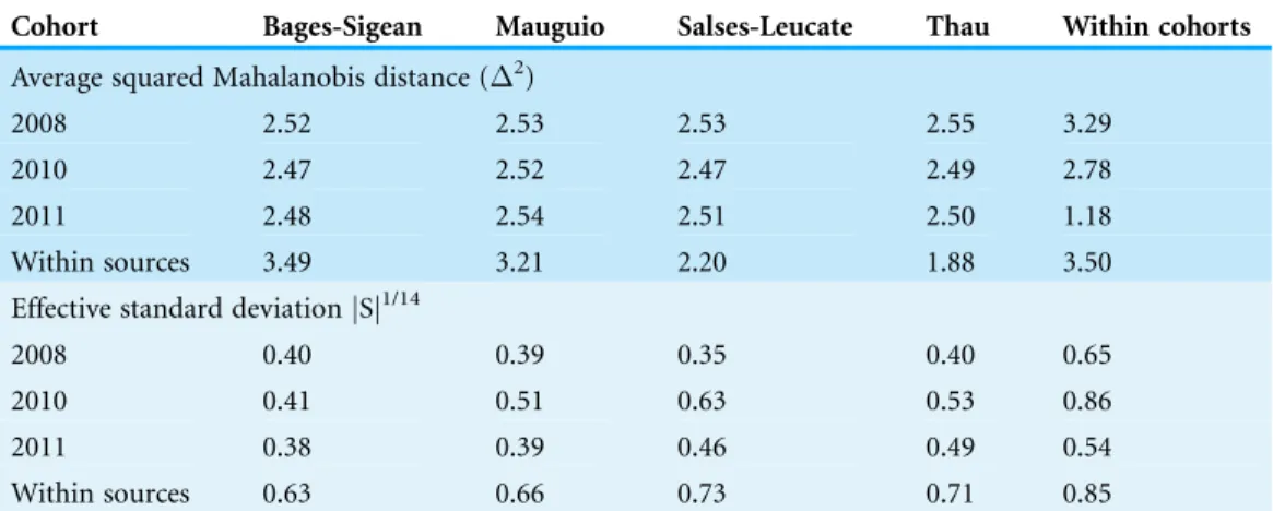
spread (effective general variance) ranged between 0.54–0.86 within the same interval (Table 1). A multivariate analysis of variance showed significant effects of cohort, nursery-source and their interaction upon these nursery signatures (p < 0.001).
Simulation approach and scenarios
All simulations and analyses were based upon the construction of two datasets: (i) a “nursery-source dataset” that represented otolith composition data from pre-migratory juveniles, sampled at their corresponding nursery-origins, and (ii) a “mixed-stock dataset” that represented otolith composition data from older fish sampled after they had mixed with fish from the other four origins (i.e. at the open sea). Besides the observed variability among the three sampled cohorts, we simulated additional variability in two dimensions: (i) the number of sources being sampled and included in the “nursery-source dataset” and/or (ii) the degree of separation among nursery-signature centroids (Table 2).
Nursery-source sampling scenarios
Five scenarios were defined by the number of sources included in the nursery-source dataset. At each run,KS= 0–4 sources were randomly selected to be included
in the nursery-source dataset as “known” nursery habitats, which had been sampled for pre-migratory juveniles. These data had been used as baseline data to produce initial estimates for^kand then mixed with the mixed-stock data to produce final^kparameters,
following an unconditional likelihood maximization approach. All remaining “unknown” nursery sources (KU= K-KS) were excluded from the nursery-source dataset and
lacked of initial ^k values.
Separation among nursery signatures
To improve our empirical understanding about the effects the separation among nursery-signature centroids may have on bias and uncertainty in ML-MM parameters, we applied the five sampling scenarios to (i) the three observed cohorts (2008, 2010 and
Table 1 Average Mahalanobis distance and effective standard deviation for elemental compositions of selected metals in otoliths of juvenileSparus aurata.Average Mahalanobis distance and effective standard deviation for elemental compositions of selected metals in otoliths of juvenileSparus aurata. Average distances within nursery source and cohort computed from vectors of observations. Average distances within years and within sources computed from vectors of means corresponding to each source or year, respectively. All values computed after standardizing all data to = 0 and = 1.
Cohort Bages-Sigean Mauguio Salses-Leucate Thau Within cohorts
Average squared Mahalanobis distance (2)
2008 2.52 2.53 2.53 2.55 3.29
2010 2.47 2.52 2.47 2.49 2.78
2011 2.48 2.54 2.51 2.50 1.18
Within sources 3.49 3.21 2.20 1.88 3.50
Effective standard deviationjSj1/14
2008 0.40 0.39 0.35 0.40 0.65
2010 0.41 0.51 0.63 0.53 0.86
2011 0.38 0.39 0.46 0.49 0.54
2011); and (ii) six virtual cohorts created to expand the range of Mahalanobis distances 2among nursery-signature centroids observed in the three sampled cohorts (2= 1.18–3.29),Table 1. To build these six virtual cohorts, covariance matrices were set equal to those estimated in 2010 for each nursery-source (Appendix 1), while the vectors of means correspondng to this same year (Appendix 1) were re-scaled to get2values of 0.5, 1.5, 2.5, 3.5, 4.5 and 5.5 (Table 2).
Resampling procedures
Datasets for each tested scenarios and independent run were produced by parametric bootstrapping. Nursery-source datasets included 25 observations drawn from each of theKSknown nursery-sources and from each of the three cohorts. Mixed-stock datasets
included a total of 100 observations per cohort, drawn from all four nursery-sources, mixed using uneven mixing proportions (m) of 0.1, 0.2, 0.3 or 0.4. These four proportions represented the true value of pk and were randomly allocated to the four
nursery-sources, within each resampling run. Resampling was followed by a standard modelling and fitting procedure, detailed inAppendix 1. This was a 12-steps sequence, which was repeated 1,000 times for each cohort and scenario. Each repetition was labelled as a “resampling run.”
Mixing proportions
To evaluate bias and uncertainty of mixing proportion estimates (^pk), we assumed the true
number of nursery sources was known and fixed (K= 4) across all scenarios. Bias in^pwas computed as the sum of the average differences between the estimated (^pmr) and the true
mixing proportion (pmr) assigned to each nursery-source within each resampling run. The
subscriptm= {0.1, 0.2, 0.3, 0.4} represents here the vector of mixing proportions
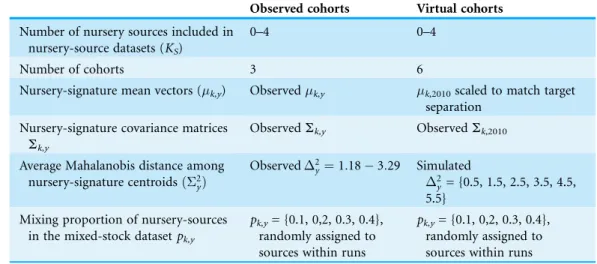
Table 2 Main configuration of the simulation and resampling procedures used for assessing the performance of maximum likelihood mixed models. Main configuration of the simulation and resampling procedures used for assessing the performance of maximum likelihood mixed models. Observed cohorts corresponded to juvenileSparus auratacollected from four Mediterranean lagoons in three highly contrasting years. Virtual cohorts corresponded to artificial data, aimed to expand the observed range of separation among nursery signatureskandysubscripts represent nursey-sources and cohorts, respectively. Observed mean vectors and covariance matrices available inAppendix 2.
Observed cohorts Virtual cohorts
Number of nursery sources included in nursery-source datasets (KS)
0–4 0–4
Number of cohorts 3 6
Nursery-signature mean vectors (k,y) Observedk,y k,2010scaled to match target separation
Nursery-signature covariance matrices Sk,y
ObservedSk,y ObservedSk,2010
Average Mahalanobis distance among nursery-signature centroidsð2
yÞ
Observed2
y¼1:18 3:29 Simulated
2
y= {0.5, 1.5, 2.5, 3.5, 4.5,
5.5} Mixing proportion of nursery-sources
in the mixed-stock datasetpk,y
pk,y= {0.1, 0,2, 0.3, 0.4}, randomly assigned to sources within runs
randomly allocated to the four nursery-sources, within each of the R = 1,000 resampling runs. Therefore,
BI^p¼
XM
m¼1 1
R
XR
r¼1
^
pmr pmr
j j
Uncertainty in^pk was indexed as the average of the four empirical standard errors
of ^pcomputed for each of the four possible values ofm, across the R = 1,000 resampling runs,
SE^p¼
1
M
XM
m¼1
ffiffiffiffiffiffiffiffiffiffiffiffiffiffiffiffiffiffiffiffiffiffiffiffiffi
ð^pmr pmrÞ2
R
s
Nursery-signature parameters
Under the assumption of multivariate normal distribution, each set of estimated nursery-signature parameters ^k was composed by a vector of means^k and a covariance matrix
^
k, which described the multivariate distribution of the seven chemical elements
measured in the otoliths included in the dataset. Assessing bias in^k is a complex task,
which we considered that exceeded the scope of this paper. Therefore, all bias measures provided hereafter for^k are strictly referred to^k.
As done for^pk, the assessment of bias and uncertainty in^was conducted assuming a
known and fixed value ofK= 4. Overall bias in^kwas indexed by averaging the absolute
mean differences between estimated (^kr) and true (kr) vectors of means, across all
elemental ratios (J= 7) and nursery-sources (K= 4). As all elemental ratios were previously standardized, bias units were equivalent to standard deviations and computed as follows,
BI^¼
1
J K
XJ
j¼1
XK
k¼1 1
R
XR
r¼1
^
kr k
Overall uncertainty in^i, was indexed by its effective standard deviation (Pen˜a &
Rodrı´guez, 2003), defined as,
SE^¼
1
K
XK
k¼1
d X k
1=2J
where, ^k is the covariance matrix computed from all^kr estimated for each
nursery-sourcekacross the R = 1,000 resampling runs.
Number of contributing nursery sources
For assessing bias and uncertainty in K^, this parameter was not set to a constant as before, but estimated by a model selection approach as described in the next section. Bias inK^ was computed asBIK^¼K^ 4, and uncertainty (SEK^) as the standard error of
^
lowest and the median Bayesian Information Criterion (BIC) values computed for all competing models, within each resampling run.
ML-MM parameter estimation
Parameters^pk and^k (^k and^k) were estimated by maximum likelihood, using the
Expectation-Maximization (EM) algorithm (Dempster, Laird & Rubin, 1977), modified to follow an unconditional approach where initial^k estimates were updated to maximize
the joint likelihood of both nursery-source and mixed-stock datasets (Appendix 1). The M-step was constrained to produce definite positive covariance matrices, with det (S) > 109. Starting^k and^k parameters for theKSknown nursery-sources were
computed directly from the nursery-source dataset. Starting ^k for theKUunknown
nursery-sources were obtained from the mixed-stock dataset trough a semi-supervised
K-means clustering procedure, implemented using the R-package “vegclust” (De Ca´ceres, Font & Oliva, 2010), which allowed for combining “fixed” and “mobile” centroids. Fixed centroids corresponded to^k estimated at the previous step for theKSknown
nursery-sources. KUadditional mobile centroids, which represented theKUunknown nursery
sources, were estimated as the values that minimized the mean square distance between the mixed-stock data and all (fixed and mobile) model centroids. Starting^k for theKU
unknown nursery-sources were computed, at a subsequent step, from the mixed-stock data clustered into each of theseKUadditional clusters (Appendix 1). Starting^pk were
calculated as the empirical proportion of individuals represented in the mixed-stock dataset assigned to each putative nursery-sourcekin order to maximize de probability density of each observation pðxij^kÞ, assumingxi MVNð^kÞ.
Parameter K^ was estimated following a model selection procedure, where multiple competing models were fit to each pair of nursery-source and mixed-stock datasets. These competing models considered a range of Kvalues, between a minimum of
Kmin= KSand a maximum defined arbitrarily as Kmax = 8. As result, within each
resampling run, and depending upon the value ofKS, a total of 4–9 competing models
were fit and compared. Model comparisons were performed usingSchwarz (1978)’s BIC, where the most informative value ofKwas addressed as the “estimated” number or nursery-sources (K^).
RESULTS
Mixing proportions
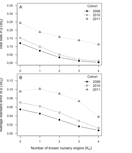
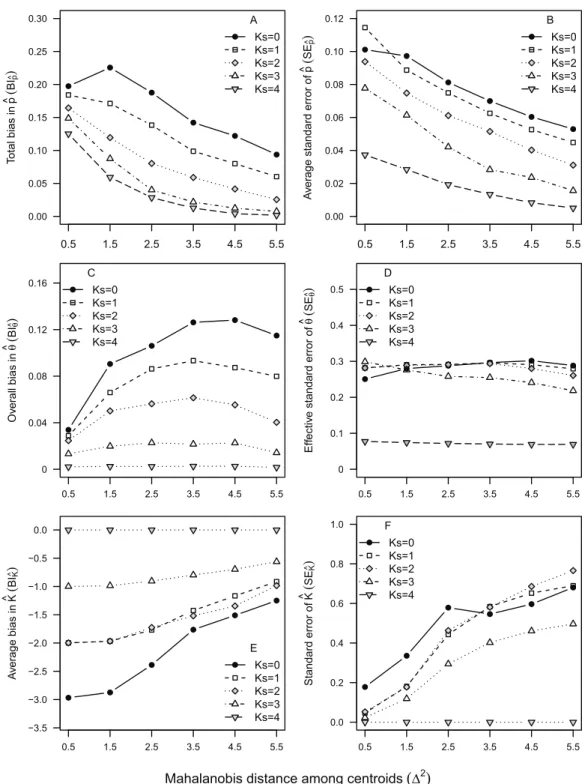
Bias in^pðBI^pÞranged between 0 and 0.24 across all data availability scenarios and observed
cohorts. Relatively unbiased^pestimatesðBI^p<0:1Þwere obtained under most data
availability scenarios (KS= 1–4) for cohorts 2008 and 2010 (Table 3;Fig. 1), but exceeded
0.11 across all scenarios for cohort 2011. The highest values ofBI^p(0.12–0.24) were found at
KS= 0, when none of the nursery-sources were known (Table 3;Fig. 1). When all
nursery-sources were known (KS= 4),BI^papproached zero for cohorts 2008 and 2010,
but remained relatively high (BI^p∼0.11) for cohort 2011. Such a decrease in bias was near
values observed for cohort 2011 (SE^p= 0.03–0.11) than for both cohort 2010 (SE^p= 0.007–
0.05) and for cohort 2008 (SE^p= 0.01–0.07). Following a pattern somewhat similar toBI^p,
we found thatSE^pdecreased rapidly asKSincreased (Fig. 1).
The rank order ofBI^p andSE^p values among the three observed cohorts was inverse
to the rank order of their average distance among nursery-signature centroids (Table 1). This inverse relationship was also observed in the six nursery-signature separation scenarios, whereBI^pandSE^pdecreased rapidly as the distance among nursery signatures
increased (Fig. 2). Such a decrease tended to evolve from a linear pattern at the worse 1–2 scenarios (KS= 0–1) to a more exponential decay pattern asKSapproached its maximum
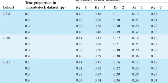
(Fig. 2) There was also an evident trend to observe positive bias at lower^p values, and negative bias at higher ^pvalues, which was more pronounced asKSdecreased (Table 3).
Nursery-signature parameters
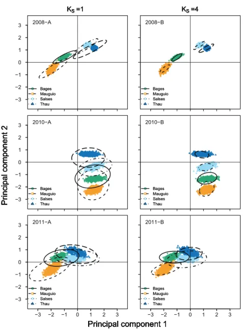
Estimated nursery-signature parameters provided relatively unbiased and consistent (similar shape and orientation) fits to the “true” distribution of means, even at theKS= 0
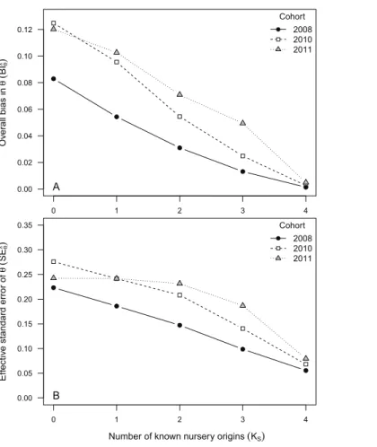
scenario (Fig. 3). Considering the observed cohorts,BI^ranged between 0.005 and 0.13 at
KS= 4 andKS= 0, respectively (Fig. 4). As observed before for mixing proportions,BI^ tended to be much higher for cohort 2011 than for cohort 2008, across all scenarios. However, the values ofBI^for cohort 2010 tended to be much closer to those computed for cohort 2011, than to the ones computed for cohort 2008 (Fig. 4). As for the six nursery-signature separation scenarios (Fig. 2),BI^tended to increase with distance from minimum values atS2= 0.5 towards maximum values and highest sensitivity to incomplete sampling 2values of 3.5 or 4.5 depending on the number of known nursery sources (Fig. 2).
Table 3 True and estimated mixing proportions of nursery-sources in the mixed-stock dataset (pk).
True and estimated mixing proportions of nursery-sources in the mixed-stock dataset (pk). Data from all nursery-sources combined for simplicity. True values corresponded to the proportion of bootstrap samples drawn from each cohort and nursery-source at each resampling runs (R = 1,000). These nursery-source proportions were assigned randomly from the vectorm= {0.1, 0.2, 0.3, 0.4}.
Cohort
True proportion in mixed-stock dataset (pk)
Sampling scenario (number of habitats represented in nursery-source datasets)
KS= 4 KS= 3 KS= 2 KS= 1 KS= 0
2008 0.1 0.10 0.10 0.11 0.13 0.15
0.2 0.20 0.20 0.20 0.21 0.21
0.3 0.30 0.30 0.30 0.29 0.29
0.4 0.40 0.40 0.39 0.37 0.35
2010 0.1 0.11 0.11 0.12 0.14 0.16
0.2 0.20 0.20 0.21 0.21 0.22
0.3 0.30 0.30 0.30 0.29 0.28
0.4 0.40 0.39 0.38 0.36 0.35
2011 0.1 0.14 0.15 0.16 0.17 0.19
0.2 0.21 0.22 0.22 0.23 0.23
0.3 0.28 0.29 0.28 0.28 0.27
Uncertainty in^kðSE^Þwas less sensitive to data availability (KS) thanBI^, showing a moderate although nearly constant decrease with KS, in cohorts 2008 and 2010. For
cohort 2011, however, SE^was similarly high betweenKS= 0 and KS = 2, decreasing
afterwards. Uncertainty in ^k tended to be higher for cohorts 2010 and 2011 than for
cohort 2008, across all scenarios, but particularly between KS= 1 and KS= 3. Results
from simulated nursery-signature separation scenarios (Fig. 2) showed SE^was not affected by distance among nursery signatures when all nursery-sources were previously known and sampled (KS = 4). Otherwise,SE^tended to decrease with distance among nursery signatures, although forKS= 0 this decrease was only evident at the two highest
distances among nursery signatures (Fig. 2).
Number of contributing nursery sources
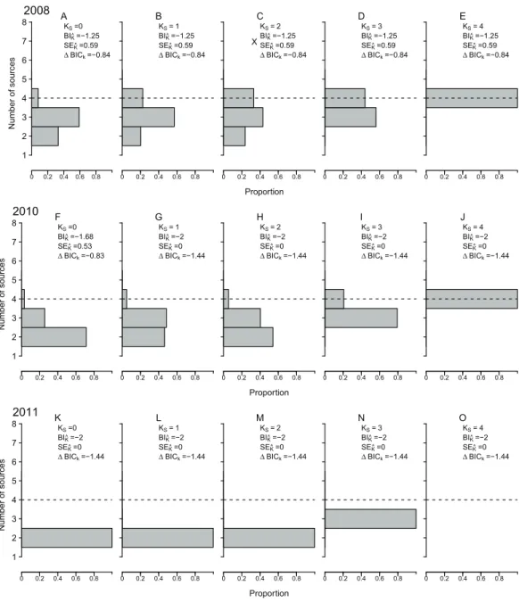
ML-MM tended to underestimate the true value ofKfor all observed cohorts, under most data availability scenarios (Fig. 5), with negative bias (BI^k), between-0.56 and-2,
across all incomplete sampling scenarios. Only under the ideal scenario (KS= 4)BI^k
●
●
●
●
●
0.00 0.05 0.10 0.15 0.20 0.25 0.30 0.35
T
o
tal bias in
p^
(
BIp^
)
0 1 2 3 4
● Cohort
2008 2010 2011
A
●
●
●
●
●
0.00 0.02 0.04 0.06 0.08 0.10 0.12
A
v
er
age standard error of
p^
(
SE
p^
)
0 1 2 3 4
● Cohort
2008 2010 2011
B
Number of known nursery origins(KS)
● ●
●
● ●
●
0.00 0.05 0.10 0.15 0.20 0.25 0.30
T
otal bias in
p^
(
BI
p^
)
0.5 1.5 2.5 3.5 4.5 5.5
●
A
Ks=0 Ks=1 Ks=2 Ks=3 Ks=4
● ●
●
●
● ●
0.00 0.02 0.04 0.06 0.08 0.10 0.12
A
v
er
age standard error of
p^
(
SE
p^
)
0.5 1.5 2.5 3.5 4.5 5.5
●
B
Ks=0 Ks=1 Ks=2 Ks=3 Ks=4
● ●
●
● ●
●
Ov
er
all bias in
θ
^ (
BI
θ
^)
0.5 1.5 2.5 3.5 4.5 5.5
0 0.04 0.08 0.12 0.16
●
C
Ks=0 Ks=1 Ks=2 Ks=3 Ks=4
●
● ●
● ●
●
Eff
e
ctiv
e standard error of
θ
^(
S
Eθ
^)
0.5 1.5 2.5 3.5 4.5 5.5
0 0.1 0.2 0.3 0.4
0.5 ●
D
Ks=0 Ks=1 Ks=2 Ks=3 Ks=4
● ●
● ●
● ●
−3.5 −3.0 −2.5 −2.0 −1.5 −1.0 −0.5 0.0
A
v
er
age bias in
K
^ ( BIK
^)
0.5 1.5 2.5 3.5 4.5 5.5
●
E
Ks=0 Ks=1 Ks=2 Ks=3 Ks=4
● ●
● ●
● ●
0.0 0.2 0.4 0.6 0.8 1.0
Standard error of
K
^(
SE
K
^)
0.5 1.5 2.5 3.5 4.5 5.5
●
F
Ks=0 Ks=1 Ks=2 Ks=3 Ks=4
Mahalanobis distance among centroids(∆2)
Figure 2 Bias and uncertainty in mixture model parameters for virtual cohorts ofSparus aurata. Average bias and uncertainty in mixing proportions ^p (A and B), nursery-signature estimates ^
became zero and the true value of Kwas correctly estimated in 100% of all simulations. Nonetheless, it must be recalled that underKS= 4,K^ was constrained to values greater or
equal toKmin= 4. As for the remaining scenarios (KS< 4), the absolute value ofBI^ktended to decrease as KSincreased, at least for cohorts 2008 and 2010 (Fig. 5).
The under-estimation ofK^ was a highly consistent pattern, observed across all nursery-signature separation scenarios, were no estimated values of K^ 5 were ever
● ●● ● ● ● ●● ● ● ● ● ●● ●● ● ● ● ●● ●● ● ● ● ● ● ● ● ● ● ●●● ● ● ● ● ● ● ● ●●● ● ● ●●●●● ● ● ● ● ● ● ● ● ●●● ● ● ●● ● ●● ● ● ●● ● ● ● ●● ●● ● ●●● ● ● ● ●●●●●● ● ●●● ● ● ● ● ● ● ● ●● ● ● ● ● ● ● ● ● ● ● ● ● ● ● ●●● ● ● ● ● ●● ●●●●● ● ●● ● ● ● ● ● ●● ● ● ● ● ● ● ● ● ●● ● ● ● ● ● ● ●● ● ●● ● ● ● ● ● ● ● ● ●● ● ● ● ● ● ● ● ● ● ● ● ● ● ● ●● ●●●●●●●●● ● ● ● ● ● ● ● ● ● ● ● ● ● ● ● ● ● ● ● ● ● ● ● ● ● ● ● ●● ● ● ● ● ● ●●● ● ● ●● ● ● ● ●● ● ● ● ● ● ● ● ● ● ● ● ● ●● ●●●● ● ●● ● ● ● ● ● ● ● ● ●●● ● ● ●●● ● ● ● ●●● ● ● ● ● ● ● ● ● ● ● ● ● ● ● ● ● ● ● ● ● ● ● ●● ● ● ●●●● ● ● ● ● ● ●●●●●● ●● ● ● ●● ● ● ●● ●● ● ● ● ● ● ● ● ● ● ● ● ● ●● ● ● ● ● ● ●● ● ● ● ● ● ● ● ● ● ● ●● ● ● ● ● ● ● ● ● ● ●● ● ● ● ● ● ● ●● ● ● ● ● ● ● ● ● ● ● ● ● ● ● ● ● ● ● ● ● ●● ● ● ● ● ● ● ●● ●● ● ●●●● ● ● ●● ● ● ● ● ●● ● ● ● ●● ● ● ● ●● ● ● ● ● ● ●● ● ● ●● ● ● ● ● ● ● ● ● ● ● ● ● ● ●●●● ● ● ●● ● ● ● ● ● ● ● ●● ● ● ●● ●●● ● ● ● ●● ●● ●● ● ● ● ● ● ● ● ● ● ● ● ●● ● ●●● ●● ●●● ●●●● ● ● ●●●●● ● ● ● ● ● ● ● ● ● ● ● ● ● ● ● ● ● ● ●●● ● ● ●● ●● ●● ● ●● ● ● ● ● ● ● ● ●● ● ●● ● ● ● ● ● ● ●● ● ● ●●● ●● ● ● ● ● ● ● ● ● ●●●● ●● ●●●● ● ● ● ● ● ● ● ● ● ● ●●●● ●● ● ● ● ● ● ● ● ●● ● ● ●● ●● ● ● ● ● ● ● ● ● ● ● ● ● ● ●● ● ●● ●● ● ● ● ● ● ● ● ●● ● ● ● ●●● ● ●● ● ● ● ● ● ● ● ● ● ● ● ● ● ● ● ● ● ● ● ●● ● ● ●● ● ● ● ● ●● ● ● ● ● ● ● ● ● ● ● ●●●●● ● ● ●● ● ● ● ●●● ● ●● ● ● ● ●●● ● ● ● ● ● ● ● ● ● ●● ● ● ●● ● ● ● ● ● ●● ● ● ● ● ● ● ● ●●●●●● ●●● ●●● ● ● ● ● ● ● ● ● ● ● ● ● ●● ●● ●● ● ● ● ● ● ● ● ● ● ●●●●● ● ● ● ● ● ●●● ● ● ●● ● ● ● ● ● ● ● ● ● ● ● ● ● ●●● ● ● ● ●●●●● ● ● ●●● ● ● ●● ● ●● ● ● ● ● ●●● ● ● ● ● ● ● ●● ● ● ● ● ● ●● ● ● ● ● ● ● ●●●●●● ● ● ● ● ● ●●●●●●● ●● ● ● ● ● ● ●● ● ● ● ● ● ●● ● ● ● ●● ● ● ● ● ● ●● ● ● ● ● ● ● ● ● ●● ●● ● ●●● ● ● ● ● ● ●● ●● ● ● ● ● ● ● ● ● ● ● ● ● ● ● ● ● ● ● ● ● ●● ● ● ● ● ● −3 −2 −1 0 1 2 3 2008−A
Principal component 1
Pr
incipal component 2
KS=1 KS=4
● Bages Mauguio Salses Thau Bages Mauguio Salses Thau ● ●● ● ● ● ●● ● ● ● ● ●● ●● ● ● ● ●● ●● ● ● ● ●● ● ● ● ● ●●● ● ● ● ● ● ● ● ●●● ● ● ●●●●● ● ● ● ● ● ● ● ● ●●● ● ● ●● ● ● ● ● ● ● ● ● ● ● ●● ●● ● ● ●● ● ● ● ●●●● ● ● ● ●●● ● ● ● ● ● ● ● ●● ● ● ● ● ● ● ● ● ● ● ● ● ● ● ●●● ● ● ● ● ●● ●●●●● ● ●● ● ● ● ● ● ●● ● ● ● ● ● ● ● ● ●●● ● ● ● ● ● ●● ●●● ● ● ● ● ● ● ● ● ●● ● ● ● ● ● ● ● ● ● ● ● ● ● ● ●● ●●●●●●●●● ● ● ● ● ●● ● ● ● ● ● ● ● ● ● ● ● ● ● ● ● ● ● ● ● ● ● ●● ● ● ● ● ● ●● ● ● ● ●● ● ● ● ●● ● ● ● ● ● ● ● ● ● ● ●● ●● ●●●● ● ●● ● ● ● ● ● ● ● ● ●●● ● ● ● ●● ● ● ● ●●● ● ● ● ● ● ● ● ● ● ● ● ● ● ● ● ● ● ● ● ● ● ● ●● ● ● ●●●● ● ● ● ● ● ●●●●●● ●● ● ● ●● ● ● ●● ●● ● ● ● ● ● ●●●●● ● ● ●● ● ● ● ● ● ●● ● ● ● ● ● ● ● ● ● ● ●● ● ● ● ● ● ● ● ● ● ●● ● ● ● ● ● ● ●● ● ● ● ● ● ● ● ● ● ● ● ● ● ● ● ● ●● ● ● ●● ● ● ● ● ● ● ● ● ●● ● ●●●● ● ● ●● ● ● ● ● ●● ● ● ● ●● ● ● ● ● ● ● ● ● ● ● ●● ● ● ●● ● ● ● ● ● ● ● ● ● ● ● ● ● ●●●● ● ● ●● ● ● ● ● ● ● ● ●● ● ● ●● ●●● ● ● ● ●● ●● ●● ● ● ● ● ● ● ● ● ● ● ●●● ● ●●● ●● ●● ● ●●●● ● ● ●●● ●● ● ● ● ● ● ● ● ● ● ● ● ● ● ● ● ● ● ● ●●● ● ● ●● ●● ●● ● ●● ● ● ● ● ● ● ● ●● ● ●● ● ● ● ● ● ● ●● ● ● ●●● ●● ● ● ● ● ● ● ● ● ● ●●●● ● ●●●● ● ● ● ● ● ● ● ● ● ● ●●●● ●● ● ● ● ● ● ● ● ●● ● ● ●● ●● ● ● ● ● ● ● ● ● ● ● ● ● ● ●● ● ●● ●● ● ● ● ● ● ● ● ●● ● ● ● ●●● ● ●● ● ● ● ● ● ● ● ● ● ● ● ● ● ● ● ● ● ● ● ●● ● ● ●● ● ● ● ● ●● ● ● ● ● ● ● ● ● ● ● ●●●●● ● ● ●● ● ● ● ●●● ● ●● ● ● ● ●●● ● ● ● ● ● ● ● ● ● ●● ● ● ●● ● ● ● ● ● ●● ● ● ● ● ● ● ● ●●●●●● ●●● ●●● ● ● ● ●● ● ● ● ● ● ●● ●● ●● ●● ● ● ● ● ● ● ● ● ● ●●● ●● ● ● ● ● ● ●●● ● ● ●● ● ● ● ● ● ● ● ● ● ● ● ● ● ●● ● ● ●● ●●●●● ● ● ●●● ● ● ● ● ● ●● ● ● ● ● ●●● ● ● ● ● ● ● ●● ● ● ●● ● ●● ● ● ● ● ● ● ●●●●●● ● ● ● ● ● ●●●●●●● ●● ● ● ● ● ● ●● ● ● ● ● ● ● ● ● ● ● ●● ● ● ● ● ● ●● ● ● ● ● ● ● ● ● ●●●● ● ●●● ● ● ● ● ● ●● ●● ● ● ● ● ● ● ● ● ● ● ● ● ● ● ● ● ● ● ● ● ●● ● ● ● ● ● 2008−B
Principal component 1
Pr
incipal component 2
KS=1 KS=4
● Bages Mauguio Salses Thau Bages Mauguio Salses Thau ● ● ● ● ● ● ●●●● ● ● ● ● ● ● ● ● ●●● ● ● ● ● ● ● ● ● ● ● ● ● ● ●●● ● ● ● ● ● ● ● ● ● ● ● ● ● ● ● ● ● ● ● ● ●● ● ● ● ● ● ●● ● ● ● ● ● ● ● ● ● ● ● ● ● ● ● ● ● ● ●● ● ●● ● ● ● ● ● ● ● ● ● ● ● ● ● ● ● ● ● ● ● ●● ● ●● ● ● ● ● ● ● ● ● ● ●● ● ● ● ● ● ● ● ● ● ● ● ● ● ●● ● ● ● ● ● ● ●● ● ●● ● ● ● ● ● ● ● ● ● ● ● ● ● ● ● ●● ●● ● ● ●● ● ● ● ● ● ● ● ● ● ● ● ● ●● ● ● ● ● ● ● ● ● ● ● ● ● ● ●●●● ● ●● ● ● ● ● ● ●● ● ● ● ● ● ● ● ● ● ● ● ●● ● ● ●● ● ● ● ● ● ● ● ●● ●● ● ●● ●● ● ● ● ● ● ● ● ● ● ●● ● ● ●● ● ● ● ● ● ● ● ● ● ●● ● ● ● ●●●● ● ● ●● ● ● ● ● ● ●●● ● ● ● ● ● ● ● ● ● ● ● ● ● ● ● ●●● ● ● ● ●● ●● ● ● ● ● ●● ● ● ● ● ●●● ● ● ●●● ● ●● ● ● ● ● ●●● ● ●● ●● ● ● ● ● ● ● ●● ● ● ● ● ● ● ● ●● ●● ● ● ● ● ● ●● ● ● ● ● ● ● ● ● ●●● ● ●●● ● ● ● ● ● ● ●● ● ● ● ●● ● ● ● ● ● ● ● ●● ● ● ● ● ●●● ● ●●●●● ● ● ● ● ● ● ● ● ● ●● ● ● ● ●●● ●● ● ●● ● ● ● ● ●●● ● ● ● ● ● ● ● ● ● ● ● ● ● ● ● ● ● ● ● ● ●●● ● ● ● ●●●●● ● ●● ● ● ● ● ● ● ●● ● ●●●●● ● ● ● ● ●●● ●●● ● ● ● ●● ● ● ● ● ● ● ● ●● ● ● ●● ● ● ●● ● ● ● ● ●●●● ● ● ● ● ● ● ● ● ● ● ● ● ● ● ● ● ● ●● ● ● ●● ● ● ●● ● ● ● ●●● ● ● ● ● ●● ● ● ● ● ●● ● ● ● ● ● ● ●●●●●● ● ● ●●● ● ● ● ● ● ● ● ● ● ● ● ● ● ● ●● ● ●● ● ● ● ● ● ● ● ● ● ● ● ● ● ● ● ● ●● ● ●● ● ● ● ● ● ● ● ● ● ● ● ● ● ●● ● ● ● ● ● ● ● ● ●●●●●●● ● ● ● ●●● ● ● ●● ● ● ● ● ●● ●● ●● ● ● ● ● ● ● ● ● ● ● ●● ●●●● ● ● ● ● ● ● ● ● ● ●●● ● ● ●● ● ●● ●● ● ●● ● ● ● ● ●● ● ● ● ● ● ● ● ● ● ● ● ● ● ● ● ● ● ● ●● ● ● ● ● ● ● ● ●● ● ● ● ● ● ● ● ● ● ● ● ● ● ● ● ●● ● ● ● ● ● ● ● ● ● ● ●● ● ● ● ● ● ● ● ● ● ●● ● ● ● ● ● ● ● ● ● ● ● ●● ● ● ● ● ● ● ● ● ● ● ● ● ● ● ● ● ● ● ● ● ● ● ● ● ● ● ● ● ● ● ●● ● ● ● ● ● ● ● ● ● ● ● ● ● ● ● ●●●● ● ● ● ● ● ● ● ● ● ● ●●●● ● ● ● ●● ● ● ●● ●●●● ●●●●●● ●● ● ● ● ● ● ● ● ● ● ●● ● ● ● ● ● ● ● ●●● ● ● ● ● ● ●●● ● ● ● ●● ● ● ●● ● ● ● ●● ● ● ● ● ● ● ● ● ● ●● ● ● ●●●● ●●●●● ● ● ●●● ● ● ● ● ● ● ●●● ● ● ● ● ● ● ● ● ● ●●● −3 −2 −1 0 1 2 3 2010−A
Principal component 1
Pr
incipal component 2
KS=1 KS=4
● Bages Mauguio Salses Thau Bages Mauguio Salses Thau ● ● ● ● ● ● ●● ●● ● ● ● ● ● ● ● ● ●●● ● ● ● ● ● ● ● ● ● ● ● ● ● ●●● ● ● ● ● ● ● ● ● ● ● ● ● ● ● ● ● ● ● ● ● ●● ● ● ● ● ●●● ● ● ● ● ● ● ● ● ● ● ● ● ● ● ● ● ● ●●● ● ●● ● ● ● ● ● ● ● ● ● ● ● ● ● ● ● ●● ● ● ●● ● ●● ● ● ● ● ● ● ● ● ● ●● ● ● ● ● ● ● ● ● ● ● ● ● ● ●● ● ● ● ● ● ● ●● ● ●● ● ● ● ● ● ● ● ● ● ● ● ● ● ● ● ●● ●● ● ● ●● ● ● ● ● ● ● ● ● ● ● ● ● ●● ● ● ● ● ● ● ● ● ● ● ● ● ● ●●●● ● ●● ● ● ● ● ● ●● ● ● ● ● ● ● ● ● ● ● ● ● ● ● ● ●● ● ● ● ● ● ● ●●● ●● ● ●● ●● ● ● ● ● ● ● ● ● ● ● ● ● ● ●● ● ● ● ● ● ● ● ● ● ●● ● ● ● ●●●● ● ● ●● ● ● ● ● ● ●●● ● ● ● ● ● ● ● ● ● ● ● ● ● ● ● ●●● ● ● ● ●● ●● ● ● ● ● ●● ● ● ● ● ●●● ● ● ●●● ● ●● ● ● ● ● ●● ● ● ●● ●● ● ● ● ● ● ● ●● ● ● ● ● ● ● ● ●● ●● ● ● ● ● ● ●● ● ● ● ● ● ● ● ● ●●● ● ●●● ● ● ● ● ● ● ●● ● ● ● ●● ● ● ● ● ● ● ● ●● ● ● ● ● ●●● ● ●●●●● ● ● ● ● ● ● ● ● ● ●● ● ● ● ●●● ●● ● ●● ● ● ● ● ●●● ● ● ● ● ● ● ● ● ● ● ● ● ● ● ● ● ● ● ● ● ●● ● ● ● ● ●●●●● ● ●● ● ● ● ● ● ● ●● ● ●●●●● ● ● ● ● ●●● ●●● ● ● ● ●● ● ● ● ● ● ● ● ●●● ● ●● ● ● ●● ● ● ● ● ●●●● ● ● ● ● ● ● ● ● ● ● ● ● ● ● ● ● ● ●● ● ● ●● ● ● ●● ● ● ● ●●● ● ● ● ● ●● ● ● ● ● ●● ● ● ● ● ● ● ●●●●●●● ● ●●● ● ● ● ● ● ● ● ● ● ● ● ● ● ● ●● ● ●● ● ● ● ● ● ● ● ● ● ● ● ● ● ● ● ● ●● ● ●● ● ● ● ● ● ● ● ● ● ● ● ● ● ●● ● ● ● ● ● ● ● ● ● ●●● ● ●● ● ● ● ●● ● ● ● ●● ● ● ● ● ●● ●● ●● ● ● ● ● ● ● ● ● ● ● ●● ●●●● ● ● ● ● ● ● ● ● ● ●●● ● ● ●● ● ●● ●● ● ●● ● ● ● ● ●● ● ● ● ● ● ● ● ● ● ● ● ● ● ● ● ● ● ● ●● ● ● ● ● ● ● ● ●● ● ● ● ● ● ● ● ● ● ● ● ● ● ● ● ● ● ● ● ● ● ● ● ● ● ● ● ●● ● ● ● ● ● ● ● ● ● ●● ● ● ● ● ● ● ● ● ● ● ● ●● ● ● ● ● ● ● ● ● ● ● ● ● ● ● ● ● ● ● ● ● ● ● ● ● ● ● ● ● ● ● ●●● ● ● ●● ● ● ● ● ● ● ● ● ● ● ●●● ● ● ● ● ● ● ● ● ● ● ● ●●●● ● ● ● ●● ● ● ●● ● ●●● ●●●●●● ●● ● ● ● ● ● ● ●● ● ●● ● ● ● ● ● ● ● ●●● ● ● ● ● ● ●●● ● ● ● ●● ● ● ●● ● ● ● ●● ● ● ● ● ● ● ● ● ● ●● ● ● ●● ●●● ●●●● ● ● ●●● ● ● ● ● ● ● ●●● ● ● ● ● ● ● ● ● ● ●●● 2010−B
Principal component 1
Pr
incipal component 2
KS=1 KS=4
● Bages Mauguio Salses Thau Bages Mauguio Salses Thau ● ● ● ● ● ● ● ● ● ● ●●●●● ● ● ● ●● ● ● ● ● ● ● ● ● ● ● ● ●● ● ● ● ● ● ● ● ● ● ● ● ● ● ● ● ● ● ● ● ● ● ● ● ● ● ● ● ● ●● ● ● ● ● ● ● ● ● ● ● ● ● ● ● ● ● ● ● ● ●● ● ● ● ● ●● ● ● ● ● ● ●● ● ● ● ●● ●● ●● ● ● ● ● ● ● ● ● ● ● ●● ● ● ● ● ● ● ● ● ● ●● ● ● ● ● ● ●● ● ● ● ● ● ● ● ● ● ● ● ● ● ● ● ● ● ● ● ● ● ● ● ● ● ● ● ●● ● ● ● ● ● ● ● ● ● ● ● ● ● ● ● ●● ● ●● ● ● ● ● ● ● ●● ● ●● ● ● ●●● ● ●● ● ● ● ●● ● ● ●● ● ● ● ● ● ● ● ● ●● ● ● ● ● ● ● ● ● ● ● ●●● ● ● ● ● ● ● ● ● ● ● ● ● ● ● ● ● ● ● ● ● ● ●● ● ● ● ● ● ●● ● ● ● ●● ●● ●● ● ● ● ● ● ● ● ●●● ● ● ● ● ● ● ● ● ● ● ● ● ● ●● ● ● ● ● ● ●● ● ●●● ● ● ● ● ● ● ● ● ● ● ● ●● ● ● ● ● ● ● ● ● ● ● ● ● ●● ● ● ● ● ● ● ● ● ● ● ● ● ● ●● ● ● ● ●● ● ● ● ● ● ● ● ● ● ● ● ● ● ● ●●●● ● ● ● ● ● ●● ● ● ● ● ● ● ● ● ● ● ● ● ● ● ● ● ● ● ● ● ● ● ● ● ● ● ● ● ●● ● ●● ● ●●●●● ●● ● ● ●● ● ●●● ● ● ● ● ● ●●●● ● ● ●●● ● ● ● ● ● ● ● ● ● ● ● ● ● ● ● ● ● ●● ● ●●●● ● ● ● ●● ● ● ● ● ● ● ● ● ● ● ● ●● ● ● ● ● ● ● ● ● ● ● ● ● ● ● ●● ● ● ● ● ● ● ● ● ● ● ● ● ● ● ● ● ● ● ● ● ● ● ● ● ● ● ● ● ● ● ● ● ●● ● ● ● ● ● ● ● ● ● ●●● ● ● ●● ● ● ●●●● ● ● ● ● ● ●● ● ● ● ● ● ● ● ● ● ● ● ● ● ● ●● ● ● ● ● ● ●● ● ● ● ● ● ● ● ● ● ● ● ● ● ● ● ● ● ● ●●● ● ● ● ● ● ● ● ● ● ● ● ● ● ● ●●●● ● ● ●● ● ● ● ● ● ● ● ● ● ● ● ● ● ● ● ● ● ● ●● ● ● ● ● ● ●● ●● ● ●● ● ● ● ● ● ● ● ● ●● ● ● ● ●● ● ● ●● ● ●● ● ● ● ● ● ● ● ● ● ● ● ● ● ● ● ● ● ● ● ● ● ● ●● ● ● ● ● ● ● ● ● ● ●● ● ● ● ●● ● ● ●●●●● ● ● ● ● ● ● ● ● ● ●● ● ●● ● ● ● ●● ● ● ● ● ● ●●●● ●● ● ● ● ● ● ● ● ● ● ● ● ● ● ● ● ●●● ● ● ● ● ● ● ● ● ● ● ● ● ● ●● ● ● ● ● ● ● ● ● ● ● ● ● ● ● ● ● ● ● ● ● ● ● ● ● ● ● ● ● ● ● ● ●● ● ● ● ●● ● ● ●●●● ● ● ● ● ● ● ● ● ● ●● ● ● ● ● ● ● ● ● ● ● ● ● ● ● ● ● ● ● ● ● ● ● ● ● ● ● ● ● ● ● ● ● ● ● ● ● ● ● ● ● ● ● ● ● ● ● ● ● ● ● ● ● ● ● ● ● ● ● ● ● ● ● ●● ● ● ● ● ● ●● ● ● ●● ● ● ● ●● ● ● ● ● ● ● ● ● ● ● ● ● ● ● ●● ● ● ● ● ● ● ● ● ● ● ● ● ● ● ● ● ● ● ● ● ● ●● ● ● ● ● ● ● ● ● ● ● ● ● ● ●● ● ● ● ● ● ● ● ● ● ●● ● ● ●
−3 −2 −1 0 1 2 3
−3 −2 −1 0 1 2 3 2011−A
Principal component 1
Pr
incipal component 2
KS=1 KS=4
● Bages Mauguio Salses Thau Bages Mauguio Salses Thau ● ● ● ● ● ● ● ● ● ● ●●●●● ● ● ● ●● ● ● ● ● ●● ● ● ● ● ● ●● ● ● ● ● ● ● ● ● ● ● ● ● ● ● ● ● ● ● ● ● ● ● ● ● ● ● ● ● ● ● ● ● ● ● ● ● ● ● ● ● ● ● ● ● ● ● ● ● ● ●● ● ● ● ● ● ● ● ● ● ● ● ●● ● ● ● ●● ● ●●● ● ● ● ● ● ● ● ● ● ● ●● ● ● ● ● ● ● ● ● ● ●● ● ● ● ● ● ●● ● ● ● ● ● ● ● ● ● ● ● ● ● ● ● ● ● ● ● ● ● ● ● ● ● ● ● ●● ● ● ● ● ● ● ● ● ● ● ● ● ● ● ● ●● ● ●● ● ● ● ● ● ● ●● ● ●● ● ● ●●● ● ● ● ● ● ● ●● ● ● ●● ● ● ● ● ● ● ● ● ●● ● ● ● ● ● ● ● ● ● ● ●●● ● ● ● ● ● ● ● ● ● ● ● ● ● ● ● ● ● ● ● ● ● ●● ● ● ● ● ● ●● ● ● ● ●● ● ● ●● ● ● ● ● ● ● ● ●●● ● ● ● ● ● ● ● ● ● ● ● ● ● ●● ● ● ● ● ● ●● ● ●●● ● ● ● ● ● ● ● ● ● ● ● ●● ● ● ● ● ● ● ● ● ● ● ● ● ●● ● ● ● ● ● ● ● ●●● ● ● ● ●●● ● ● ●● ● ● ● ● ● ● ● ● ● ● ● ● ● ● ●●●● ● ● ● ● ● ●● ● ● ● ● ● ● ● ● ● ● ● ● ● ● ● ● ● ● ● ● ● ● ●● ● ● ● ● ● ● ● ●● ● ●●●●● ●● ● ● ● ● ● ●●● ● ● ● ● ● ●●●● ● ● ●●● ● ● ● ● ● ● ● ● ● ● ● ● ● ● ● ● ● ●● ● ●●●● ● ● ● ●● ● ● ● ● ● ● ● ● ● ● ● ●● ● ● ● ● ● ● ● ● ● ● ● ● ● ● ●● ● ● ● ● ● ● ● ● ● ● ● ● ● ● ● ● ● ● ● ● ● ● ● ● ● ● ● ● ● ● ● ● ●● ● ● ● ● ● ● ● ● ● ●●● ● ● ●● ● ● ●●●● ● ● ● ● ● ●● ● ● ● ● ●● ● ● ● ● ● ● ● ● ●● ● ● ● ● ● ●● ● ● ● ● ● ● ● ● ● ● ● ● ● ● ● ● ● ● ●●● ● ● ● ● ● ● ●●● ● ● ● ● ● ●●●● ● ● ●● ● ● ● ● ● ● ● ● ● ● ● ● ● ● ● ● ● ● ●● ● ● ● ● ● ●● ●● ● ●● ● ● ● ● ● ● ● ● ●● ● ● ● ●● ● ● ●● ● ●● ● ● ● ● ● ● ● ● ● ● ● ● ● ● ● ● ● ● ● ● ● ● ●● ● ● ● ● ● ● ● ● ● ●● ● ● ● ●● ● ● ●●●●● ● ● ● ● ● ● ● ● ● ●● ● ● ● ● ● ● ●● ● ● ● ● ● ●●●● ●● ● ● ● ● ● ● ● ● ● ● ● ● ● ● ● ●●● ● ● ● ● ● ● ● ● ● ● ● ● ● ●● ● ● ● ● ● ● ● ● ● ● ● ● ● ● ● ● ● ● ● ● ● ● ● ● ● ● ●● ● ● ● ●● ● ● ● ●● ● ● ● ●●● ● ● ● ● ● ● ● ● ● ●● ● ● ● ● ● ● ● ● ● ● ● ● ● ● ● ● ● ● ● ● ● ● ● ● ● ● ● ● ● ● ● ● ● ● ● ● ● ● ● ● ● ● ● ● ● ● ● ● ● ● ● ● ● ● ● ● ● ● ● ● ● ● ●● ● ● ● ● ● ● ● ● ● ●● ● ● ● ●● ● ● ● ● ● ● ● ● ● ● ● ● ● ● ●● ● ● ● ● ● ● ● ● ●● ● ● ● ● ● ● ● ● ● ● ● ●● ● ● ● ● ● ● ● ● ● ● ● ● ● ●● ● ● ● ● ● ● ● ● ● ●● ● ● ●
−3 −2 −1 0 1 2 3
2011−B
Principal component 1
Pr
incipal component 2
KS=1 KS=4
● Bages Mauguio Salses Thau Bages Mauguio Salses Thau
obtained, regardless of the data availability scenario or cohort (Fig. 2). Nonetheless, the magnitude of this bias decreased by 50–70% as the distance among nursery signatures increased (Fig. 2). Uncertainty inK^(SEK^) was zero atKS= 4, but relatively high
(SEK^ > 0.4) in cohorts 2008 and 2010 for allKS< 4, reaching maximum values atKS= 2
(Fig. 5). The strength of the model selection measured byBICK tended to increase
towardsKS= 4, where it was maximum for cohorts 2008 and 2010 (Fig. 5). The consistent,
although biased, values ofK^(BIK^ = 1–2) lead to particularly low values ofSEK^ for cohort 2011, across all scenarios. Consistent values ofSEK^ ≈0 atKS= 4, and a weak
relationship betweenKSandSEK^ for allKS< 4 were observed across all nursery-signature
separation scenarios. Nonetheless, it was evident thatSEK^ tended to increase with distance among nursery signatures for all incomplete sampling scenarios.
DISCUSSION
In this article, we combined real-world and virtual datasets to evaluate the performance of unconditional ML-MM when used to estimate the three fundamental sets of mixed stock parameters (pk,kandK), under a range of data availability and distance
●
●
●
●
● 0.00
0.02 0.04 0.06 0.08 0.10 0.12
Ov
er
all bias in
θ
^(
BI
θ
^)
0 1 2 3 4
●
Cohort 2008 2010 2011
A
●
●
●
●
●
0.00 0.05 0.10 0.15 0.20 0.25 0.30 0.35
Eff
e
ctiv
e standard error of
θ
^(
SE
θ
^)
0 1 2 3 4
●
Cohort 2008 2010 2011
B
Number of known nursery origins(KS)
among nursery-signature scenarios. Although using a single real-world dataset might limit the generalization of our results, which may not be transferable to other stocks, we believe the large variability observed among cohorts in the real-world dataset, along with the additional variability included in the simulated datasets might represent a relevant part of the variability that could be found in other populations
and geographical areas.
X
Number of sources
1 2 3 4 5 6 7 8
0 0.2 0.4 0.6 0.8
A
2008
KS=0 BIK^=−1.25 SEK^=0.59 ∆ BICk=−0.84
0 0.2 0.4 0.6 0.8
B
KS=1 BIK^=−1.25 SEK^=0.59 ∆ BICk=−0.84
0 0.2 0.4 0.6 0.8
C
KS=2 BIK^=−1.25 SEK^=0.59 ∆ BICk=−0.84
0 0.2 0.4 0.6 0.8
D
KS=3 BIK^=−1.25 SEK^=0.59 ∆ BICk=−0.84
0 0.2 0.4 0.6 0.8
E
KS=4 BIK^=−1.25 SEK^=0.59 ∆ BICk=−0.84
Proportion
Number of sources
1 2 3 4 5 6 7 8
0 0.2 0.4 0.6 0.8
F
2010
KS=0 BIK^=−1.68 SEK^=0.53 ∆ BICk=−0.83
0 0.2 0.4 0.6 0.8
G
KS=1 BIK^=−2 SEK^=0 ∆ BICk=−1.44
0 0.2 0.4 0.6 0.8
H
KS=2 BIK^=−2 SEK^=0 ∆ BICk=−1.44
0 0.2 0.4 0.6 0.8
I
KS=3 BIK^=−2 SEK^=0 ∆ BICk=−1.44
0 0.2 0.4 0.6 0.8
J
KS=4 BIK^=−2 SEK^=0 ∆ BICk=−1.44
Proportion
Number of sources
1 2 3 4 5 6 7 8
0 0.2 0.4 0.6 0.8
K
2011
KS=0 BIK^=−2 SEK^=0 ∆ BICk=−1.44
0 0.2 0.4 0.6 0.8
L
KS=1 BIK^=−2 SEK^=0 ∆ BICk=−1.44
0 0.2 0.4 0.6 0.8
M
KS=2 BIK^=−2 SEK^=0 ∆ BICk=−1.44
0 0.2 0.4 0.6 0.8
N
KS=3 BIK^=−2 SEK^=0 ∆ BICk=−1.44
0 0.2 0.4 0.6 0.8
O
KS=4 BIK^=−2 SEK^=0 ∆ BICk=−1.44
Proportion
Figure 5 Estimated number of contributing sources. Estimated number of nursery-sources (K^) contributing to simulated mixed-stock ofSparus aurataobtained following a model selection approach based on Bayesian Selection Criterion. Different sampling scenarios were represented by the number of nursery-sources (KS) simulated to be known and sampled for pre-migratory juveniles. Relative fre-quencies computed after 1,000 resampling runs per tested scenario.BIK^= mean bias forK^;SEK^= mean
standard error of K^; BICK = difference between minimum and median values of the Bayesian
Mixing proportions estimated by ML-MM (^pk) showed low bias and variability when
at least one nursery source was included in the nursery-source dataset. Large variability in bias and uncertainty of ^pk was found, however, among cohorts, with cohort 2011
exhibiting the highest bias and uncertainty values in^pk. This variability in bias and uncertainty among cohorts was consistent with inter-annual differences in sensitivity to incomplete sampling resulting from variable degrees of separation among nursery signatures. Results from simulations showed, for instance, that a minimum of three sampled nursery sources had been required to reduceBI^pbelow 0.1, given a Mahalanobis
distance among nursery-signature centroids1.5.
Overall our results confirmed the suitability of using ML-MM for estimating unbiased mixing proportions, given the number of nursery-sources (K) was known and there was a proper balance between the number of sources sampled for prior nursery-signature parameters and the actual degree of separation among nursery-nursery-signature centroids. Although results from our simulated separation scenarios cannot be turn into a prescriptive guideline, they explore such trade-offs and provide a general idea about which combinations might work, at least for Mediterranean stocks of S. aurata.
When incomplete sampling and/or reduced distance among nursery signatures biased mixing proportions estimates, bias tended to be greater for the most extreme^pk values,
which were shifted towards intermediate values. Therefore, the smallest nursery contributions tended to be overestimated, while the largest ones to be underestimated. This behaviour is probably related to the model constrain that all proportions must sum one, which limits the parameter space and tend to increase negative correlation between the two most extreme values. It might be also somewhat related to the EM algorithm, which may converge to unsatisfactory local maxima (Marin, Mengersen & Robert, 2005).
Nursery-signature parameter estimates were relatively unbiased for all evaluated cohorts, under most data availability scenarios. When two or more nursery-sources were known and previously sampled,BI^dropped below 0.10. Uncertainty in^k, however, was
relatively high under incomplete sampling scenarios, particularly in cohorts 2010 and 2011, whereSE^exceeded 0.20 at allKS< 3 scenarios. The important differences in bias
and uncertainty we found among cohorts, were likely related to large environmental variability in the study area (Tournois et al., 2013), which were reflected in highly variable distribution patterns of nursery signatures among cohorts (Fig. 3). Simulated nursery-signature separation scenarios showed a dome-shaped relationship betweenBI^and distance among nursery-signature centroids, with maximum bias at intermediate distances and minimum bias at the shortest distance we tested (2= 0.5). This counter-intuitive pattern may have emerged from the antagonistic effects of less separable nursery signatures but more constrained parameter spaces at shorter distances among their centroids.
Unlike what we found for^pkand^k, the performance of our model selection approach
that enhancing our knowledge about the minimum number of contributing sources had reduced the risk of underestimating K. Given this biasing trend, the model selection approach we followed provided a lower bound rather than an accurate estimate ofK.
Exploratory comparisons (not shown in results) between BIC and Akaike (1973)’s Information Criteria (AIC) yielded results that agreed with the idea that BIC produces underestimated but less variable estimates ofK, while the opposite would be true for AIC (Koehler & Murphree, 1988). Alternative model selection criteria have been proposed by several authors and deserve further testing under a greater range of scenarios (Celeux & Soromenho, 1996). Departing from model selection approaches, bootstrapping has been proposed and used to evaluate consistency inK^ (McLachlan & Peel, 2004).Neubauer, Shima & Swearer (2013)followed, instead, a Bayesian approach to internalize the estimation ofKinto a Dirichlet process mixture model, which had the advantage of producing marginal distributions over a range of plausible K^ values and allowed for a direct probabilistic interpretation of model results. There is, however, a generalized view that estimatingKis one of the most difficult tasks within MM, for which more satisfactory solutions are still needed (Celeux & Soromenho, 1996;McLachlan & Peel, 2004; White et al., 2008;Neubauer, Shima & Swearer, 2013).
Although we focused on testing the performance of unconditional ML-MM, we must acknowledge the growing importance of Bayesian approaches, observed in relatively recent years (Pella & Masuda, 2001;Marin, Mengersen & Robert, 2005;Munch & Clarke, 2008;White et al., 2008;Smith & Campana, 2010;Standish, White & Warner, 2011;Neubauer, Shima & Swearer, 2013). They represent obvious alternatives to
conventional ML-MM which may be particularly advantageous for considering missing or incomplete data scenarios. Other approaches used for estimating mixing proportions under partial or complete lack of nursery-source data have been based upon unsupervised clustering followed by discriminant analysis (Arkhipkin, Schuchert & Danyushevsky, 2009; Shima & Swearer, 2009;Schuchert, Arkhipkin & Koenig, 2010). Nonetheless, no
independent assessments of bias or uncertainty seem to be available for this clustering approaches when applied to mixed stock analysis under incomplete sampling scenarios.
It is important to acknowledge that we did not explore sample size effects, but used constant sample sizes of 25 individuals per known nursery-source and 100 individuals per mixed-stock and cohort. While no major changes in bias would be expected at different sample sizes, an obvious reduction in uncertainty would be expected if the number of fish included in the nursery-source and/or mixed-stock datasets were larger. It would be of particular interest to consider intermediate scenarios where some small level of sampling existed for some/all nursery-sources, which maybe a common real-life situation when juvenile sampling is rather opportunistic. Under the unconditional approach we have followed, these pieces of information could be used without the risk of giving them full weight, as it would occur if they were used for producing fixed nursery-signature parameters, under the conditional approach. Moreover, these data, although limited, could be used to sustain some resampling procedures aimed to explore the risk of biased conclusions under plausible scenarios, as done in the present work.
In conclusion, unconditional ML-MM showed to be a suitable tool for estimating mixing proportions and nursery signatures of S. aurataunder multiple scenarios that included incomplete sampling and a range of chemical signature separations among nursery-sources. In contrast, our approach yielded rather discouraging results regarding the estimation of the true number of nursery-sources (K), under incomplete sampling and/or identification of nursery-sources. Therefore, new efforts aimed to develop new mixed-stock analysis tools and/or to evaluate the performance of the existing ones are required. Such evaluations should be conducted over the widest possible range of species, habitats and biological scenarios, both to improve the reliability of these tools and to enhance our understanding about the structure and connectivity of exploited and threatened fish populations.
ACKNOWLEDGEMENTS
Numerical simulations were conducted at the Chilean National Laboratory for High Performance Computing NLHPC (ECM-02). Data was kindly provided by Jennifer Tournois.
ADDITIONAL INFORMATION AND DECLARATIONS
Funding
Research was funded by the Chilean Commission for Science and Technology
(CONICYT) through FONDECYT grant No. 1131143. Otolith collection and analysis was partially funded by the TOTAL Foundation and the French ANR LAGUNEX project (07-JCJC-0135). The funders had no role in study design, data collection and analysis, decision to publish, or preparation of the manuscript.
Grant Disclosures
The following grant information was disclosed by the authors:
Chilean National Laboratory for High Performance Computing NLHPC: ECM-02. TOTAL Foundation and the French ANR LAGUNEX project: 07-JCJC-0135.
Competing Interests
The authors declare that they have no competing interests.
Author Contributions
Edwin J. Niklitschek conceived and designed the experiments, performed the experiments, analyzed the data, wrote the paper, prepared figures and/or tables, reviewed drafts of the paper.
Audrey M. Darnaude conceived and designed the experiments, contributed reagents/materials/analysis tools, wrote the paper, reviewed drafts of the paper.
Data Deposition
The following information was supplied regarding data availability: Niklitschek, Edwin (2016): three_years_data_elemental_ratio.csv. Figshare:https://dx.doi.org/10.6084/m9.figshare.2067789.v1.
Supplemental Information
Supplemental information for this article can be found online athttp://dx.doi.org/ 10.7717/peerj.2415#supplemental-information.
REFERENCES
Akaike H. 1973.Information theory and an extension of the maximum likelihood principle. In: Petrov BN, Caski F, eds.Second International Symposium on Information Theory. Budapest: Akademiai Kaido, 267–281.
Arkhipkin AI, Schuchert PC, Danyushevsky L. 2009.Otolith chemistry reveals fine population structure and close affinity to the Pacific and Atlantic oceanic spawning grounds in the migratory southern blue whiting (Micromesistius australis australis).Fisheries Research
96(1–2):188–194DOI 10.1016/j.fishres.2008.11.002.
Bolker BM, Brooks ME, Clark CJ, Geange SW, Poulsen JR, Stevens MHH, White JSS. 2009.
Generalized linear mixed models: a practical guide for ecology and evolution.Trends in
Ecology & Evolution24(3):127–135DOI 10.1016/j.tree.2008.10.008.
Barnett-Johnson R, Pearson TE, Ramos FC, Grimes CB, MacFarlane RB. 2008.Tracking natal origins of salmon using isotopes, otoliths, and landscape geology.Limnology and Oceanography
53(4):1633–1642DOI 10.4319/lo.2008.53.4.1633.
Box GEP, Cox DR. 1964.An analysis of transformations.Journal of the Royal Statistical
Society Series B (Methodological)26(2):211–252.
Campana SE, Chouinard GA, Hanson JM, Fre´chet A, Brattey J. 2000.Otolith elemental fingerprints as biological tracers of fish stocks.Fisheries Research46(1–3):343–357
DOI 10.1016/S0165-7836(00)00158-2.
Campana SE, Thorrold SR. 2001.Otoliths, increments, and elements: keys to a comprehensive understanding of fish populations?Canadian Journal of Fisheries and Aquatic Sciences
58(1):30–38DOI 10.1139/f00-177.
Cassie RM. 1954.Some uses of probability paper in the analysis of size frequency distributions.