Metabolomic Method: UPLC-q-ToF Polar and
Non-Polar Metabolites in the Healthy Rat
Cerebellum Using an In-Vial Dual Extraction
Amera A. Ebshiana1☯, Stuart G. Snowden2☯, Madhav Thambisetty3, Richard Parsons1, Abdul Hye2, Cristina Legido-Quigley1*
1Institute of Pharmaceutical Sciences, King’s College London, Franklin-Wilkins Building, 150 Stamford Street, London, SE1 9NH, United Kingdom,2Institute of Psychiatry, Department of Old Age Psychiatry, King’s College London, De Crespigny Park, London, SE5 8AF, United Kingdom,3Clinical and Translational Neuroscience Unit, Laboratory of Behavioural Neuroscience, National Institute on Aging, Baltimore, Maryland, United States of America
☯These authors contributed equally to this work.
*cristina.legido_quigley@kcl.ac.uk
Abstract
Unbiased metabolomic analysis of biological samples is a powerful and increasingly com-monly utilised tool, especially for the analysis of bio-fluids to identify candidate biomarkers. To date however only a small number of metabolomic studies have been applied to studying the metabolite composition of tissue samples, this is due, in part to a number of technical challenges including scarcity of material and difficulty in extracting metabolites. The aim of this study was to develop a method for maximising the biological information obtained from small tissue samples by optimising sample preparation, LC-MS analysis and metabolite identification. Here we describe an in-vial dual extraction (IVDE) method, with reversed phase and hydrophilic liquid interaction chromatography (HILIC) which reproducibly mea-sured over 4,000 metabolite features from as little as 3mg of brain tissue. The aqueous phase was analysed in positive and negative modes following HILIC separation in which 2,838 metabolite features were consistently measured including amino acids, sugars and purine bases. The non-aqueous phase was also analysed in positive and negative modes following reversed phase separation gradients respectively from which 1,183 metabolite features were consistently measured representing metabolites such as phosphatidylcho-lines, sphingolipids and triacylglycerides. The described metabolomics method includes a database for 200 metabolites, retention time, mass and relative intensity, and presents the basal metabolite composition for brain tissue in the healthy rat cerebellum.
Introduction
The brain is the centre of the nervous system in all vertebrates, and is responsible for controlling all bodily functions ranging from walking and talking, to heart rate and endocrine function. In addition to this diseases of the brain and central nervous system represent a major cause of
OPEN ACCESS
Citation:Ebshiana AA, Snowden SG, Thambisetty M, Parsons R, Hye A, Legido-Quigley C (2015) Metabolomic Method: UPLC-q-ToF Polar and Non-Polar Metabolites in the Healthy Rat Cerebellum Using an In-Vial Dual Extraction. PLoS ONE 10(4): e0122883. doi:10.1371/journal.pone.0122883
Academic Editor:Damir Janigro, Cleveland Clinic, UNITED STATES
Received:October 3, 2014
Accepted:February 24, 2015
Published:April 8, 2015
Copyright:This is an open access article, free of all copyright, and may be freely reproduced, distributed, transmitted, modified, built upon, or otherwise used by anyone for any lawful purpose. The work is made available under theCreative Commons CC0public domain dedication.
Data Availability Statement:All relevant data are within the paper and its Supporting Information files.
Funding:This work has been supported by grants from the Butterfield Trust and the Libyan Cultural Bureau London. The funders had no role in study design, data collection and analysis, decision to publish, or preparation of the manuscript.
global morbidity and mortality, with over 600 recognised neurological diseases [1] including de-velopmental disorders such as Down syndrome and autism spectrum disorders [2–3], seizure disorders like epilepsy [4] and neurodegenerative disorders including Alzheimer’s and Parkin-sons diseases [5–8]. Despite the importance of the brain and the pathological burden associated with it, we are still relatively ignorant of its mechanisms and it is hoped that developing a better understanding of cerebral metabolism will help to begin unlocking the secrets of the brain. Argu-ably, the biggest challenges of working with both human and animal brain tissue are twofold, firstly the small amounts/preciousness due to inaccessibility of sample material and secondly re-producible extraction of metabolites from the sample tissues. These obstacles make the develop-ment of analytical approaches that maximise the metabolites that can be reproducibly measured from small tissue samples an important challenge.
Metabolomics is the unbiased analysis of the composition of small molecule metabolites in a given biological tissue or fluid, under a specific set of environmental conditions [9–10]. Due to the wide range of concentrations at which these metabolites are present and their diverse physiochemical properties it is challenging to obtain comprehensive analysis of all metabolite classes using a single method [11–14]. Therefore many metabolomic approaches that aim to maximise metabolite coverage utilise a combination of analytical platforms including liquid chromatography—mass spectrometry (LC-MS), nuclear magnetic resonance (NMR) and gas chromatography—mass spectrometry (GC-MS) [11,15–16]. These multi-platform approaches will measure metabolites with a wide range of concentrations and physiochemical properties, however the downside to increasing metabolite coverage will be a significant increase in the amount of tissue required.
LC-MS is one of the most widely used analytical techniques for metabolite fingerprinting and has been used to analyse a range of metabolite classes in a variety of biological matrices [17–20]. One of the major advantages of this approach is that it separates complex sample mix-tures into its constituent components prior to mass spectral analysis. Separation enables the discrimination of some isobaric compounds which mass spectrometry alone cannot do, it also helps to reduce matrix effects in the ionisation chamber such as ionisation suppression in which different components of the matrix compete to be ionised resulting in a suppressed me-tabolite signal and incorrect meme-tabolite quantitation [21–24]. However, one important limita-tion is that physiochemical properties of metabolites are diverse, and a single chromatographic technique cannot separate thousands of metabolites. For example reversed phase chromatogra-phy will separate non-polar metabolites such as lipids, but not separate polar compounds like amino acids [13]. This means that all of the polar metabolites will co-elute at the start of the chromatogram, with many not being measured correctly due to ion suppression. Therefore, as a result multiple chromatographic separation techniques are required to achieve a broad cover-age of the metabolome. Sample preparation for LC-MS metabolite fingerprinting usually in-volves a solvent based (usually methanol, ethanol or acetonitrile) protein precipitation [25] to reduce surface absorption and protein-metabolite interactions. Different chromatographic conditions require distinct sample preparations increasing analysis time, analytical variability and the amount of sample material required. A main obstacle in metabolomics is metabolite identification, metabolite features measured need to be translated to chemical identities or me-tabolites that can give biological information.
Metabolite annotation has repeatedly been identified as a significant bottleneck in mass spectrometry untargeted workflows [26–27]. There are several challenges that make metabolite annotation difficult, the first of which is that there is up to an estimated 200,000 distinct metab-olites [10] less than 50% of which have been structurally identified. Many metabolites, especial-ly esoteric compounds, have unknown structure, so complete identification can onespecial-ly be done by compound synthesis, hence sharing of in-house databases is unusual. Secondly whilst does not alter the authors' adherence to all the PLOS
fragmentation patterns are used for identification, this is an expert field and good quality frag-mentation is not always possible.
To date there has been a number of metabolomic studies that have looked at the metabolite composition of brain tissue. Saleket al. [28] used 1H-NMR to measure the metabolite
compo-sition in the hippocampus, cortex, frontal cortex, midbrain and cerebellum of CRND8 mice identifying 23 metabolites from tissue samples ranging in mass from 10–50mg. In humans, brain tissue is in short supply and to date only small numbers (n = 10–15) with reversed phase fingerprinting have been profiled. However two groups were able to make important contribu-tions, Grahamet al. [29] used5g of human post mortem brain and UPLC-ToF to develop a method that detected 1,264 metabolic features, with 10 features shown to be correlated to AD. Koichiet al. [30] also used UPLC-ToF metabolomics of human brain and found spermine and
spermidine to be increased in AD pathology.
Therefore, this study aimed to obtain both polar and non-polar metabolites from a single small sample of brain tissue. For this HILIC together with reversed phase (RP) methods were investigated. Another aim was to provide the means for metabolite identification with the method, the data generated is the basal metabolome in rat cerebellum that can be applied in clinical investigations.
Materials and Methods
Chemicals and Reagents
All solvents, water, methanol, acetonitrile, ammonium formate, formic acid and methyl tertiary butyl ether (MTBE), were LC-MS grade purchased from Sigma-Aldrich. Four internal stan-dards, heptadecanoic acid (98% purity), tripentadecanoin (98% purity) for the reversed phase, and L-serine13C315N (95%) and L-valine13C515N (95%) for HILIC were purchased from Sigma-Aldrich. In-vial dual extractions were performed in amber glass HPLC vials with fixed 0.4 mL inserts (Chromacol: Welwyn Garden City, UK).
Samples
Experimental tissue material was obtained from the cerebellum of adult male (Sprague-Daw-ley) rats obtained from Harlan Laboratories UK. The animals were euthanized in the Biomedi-cal services unit, King’s College London by inducing carbon dioxide (CO2) anoxia followed by cervical dislocation as per Schedule 1 of the Animal (scientific procedures) Act of 1986. All ani-mal procedures were approved by local aniani-mal welfare and the Ethics Review Body (King’s College London). The cerebellum was isolated according to the Springer protocol for the dis-section of rodent brain regions [31], samples were weighed and subsequently stored at -80°C. The cerebellum was sectioned on sterile glass slides (Thermo Scientific, Menzel-Glazer slides) using a sterile scalpel, both scalpel and slide were cooled in liquid nitrogen to reduce sample thawing during sectioning. Sectioned tissue samples were transferred to Eppendorf tubes con-taining a clean, pre-cooled, 5mm stainless steel ball bearing.
Experimental Design
extractions prior to injection on both HILIC and reversed phase methods (Fig 1A). The second experiment was designed to assess the effect of the mass of tissue extracted and tissue homege-nistation on method sensitivity and precision. Four Sprague-Drawly rat brain were obtained and this material was used to perform Experiment 2. To do this 15 tissue samples ranging from 3–17mg were homogenised and extracted in parallel prior to analysis (Fig 1B). Sensitivity was assessed in terms of the number of metabolite features that are routinely detected, whilst preci-sion will be assessed in terms of the variability (coefficient of variation) of the abundance of in-ternal standard and metabolite peaks as well as the degree of compositional similarity between samples as determined principal component analysis (PCA). A graphical description of the an-alytical workflow used in this study is shown inFig 2.
Tissue homogenisation
Prior to homogenisation 20μl of methanol and 5μl of HILIC internal standard cocktail (2.5mM L-serine13C315N and L-valine13C515N in methanol:water (4:1)) was added per milligram of sample material. The tissue was then homogenised using a Tissuelyzer(Qiagen) in 10 cycles of 30 seconds at 25 Hz, subsequently a 50ul aliquot of homogenate was transferred to a Chroma-col HPLC vial (400μl fixed insert).
Fig 1. Graphical representation of the experimental designs used.A) experiment 1, a single 18mg brain section was homogenised then 7 parallel extractions were performed on 50μl aliquots of homogenate. B) Experiment 2, brain sections ranging from 3–17mg were homogenised and extracted parallel.
In-vial dual extraction of brain tissue
Subsequently 10μl of water was added to the homogenate, vials were then vortexed for 5 min-utes, after which 250μl of MTBE containing Tripentadecanoin (10μg/ml) and Heptadecanoic acid (10μg/ml) was added after which samples were again vortexed at room temperature for 60 minutes. Following the addition of a further 40μl of water containing 0.15mM ammonium formate to enhance phase separation, samples were then centrifuged at 2500×g for 30 minutes at 4°C. This resulted in a clear separation of MTBE (upper) and aqueous (lower) phases, with protein precipitate aggregated at the bottom of the vial. Quality control samples were created by pooling excess tissue homogenate from biological samples (after a 50μl aliquot had been taken), this excess homogenate was then split into 50μl aliquots for in-vial extraction.
LC-MS analysis of IVDE non-aqueous phase
LC-MS analysis was performed on a Waters Acquity ultra performance liquid chromatogram (UPLC) system coupled to a Waters Premier quadrupole time-of-flight (Q-Tof) mass spec-trometer (Waters, Milford, MA, USA). The needle height in the auto-sampler was set to 13mm, with 5μl of sample extract injected onto an Agilent Poroshell 120 EC-C8 column (150mm × 2.1mm, 2.7μm). Separation was performed at 55°C with a flow-rate of 0.5 ml/min using 10mM ammonium format in water (mobile phase A) and 10mM ammonium format in
Fig 2. Applied analytical pipeline.Shows the seven steps from tissue sectioning to IVDE and onto data processing and multivariate analysis of variation.
methanol (mobile phase B). For analysis in the positive mode, the gradient started at 80% mo-bile phase B increasing linearly to 96% B in 23 minutes and was held until 45 minutes then the gradient was increased to 100% by 46 minutes until 49 minutes. Initial conditions were re-stored in 2 minutes ahead of 7 minutes of column re-equilibration. For analysis in the negative ionisation mode the gradient started at 75% B increasing linearly to 96% B at 23 minutes, then increasing further to 100% B by 35 minutes, initial conditions were restored to allow 7 minutes of column re-equilibration. In the positive mode, a capillary voltage of 3.2 kV and a cone volt-age of 45V was applied. Data was collected between 50 and 1000m/z, the desolvation gas flow
was 400 L/hour and the source temperature was 120°C. In the negative mode, a capillary volt-age of 2.6 kV and a cone voltvolt-age of 45 V were used. Desolvation gas flow and source tempera-ture were fixed at 800 L/h and 350°C, respectively. All analyses were acquired using the lock spray to ensure accuracy and reproducibility; A reference solution (leucine-enkephalin) was used as lock mass (m/z556.2771 and 278.1141) at a concentration of 200 ng/mL to update
ac-curate mass data values and a flow rate of 10μL/min. Data were collected in the centroid mode over the mass rangem/z50–1000 with an acquisition time of 0.1 seconds a scan.
LC-MS analysis of IVDE aqueous phase
The auto sampler needle height was set at 2mm, with analysis of 5μl of aqueous phase extract being analysed on a Merck Sequant Zic-HILIC column (150 × 4.6mm, 5μm particle size) cou-pled to a Merck Sequant guard column (20 × 2.1mm). A 40 minute room temperature gradient (0.3ml/min) was applied using 0.1% formic acid in water (mobile phase A) and 0.1% formic acid in acetonitrile (mobile phase B). The gradient started at 80% mobile phase B, followed by a linear reduction to 20% mobile phase B after 30 minutes, initial conditions were restored to allow 10 minutes of column re-equilibration. Mass spectral data was acquired between 75– 1000 Daltons in both positive and negative ionisation modes. The applied mass spectrometry conditions were the same as for the reversed phase method.
Data processing and metabolite identification
The generated data was processed using MarkerLynx (Masslynx 4.1 Waters, USA) which pro-vides automated peak detection based on peak alignment and normalization to total peak area. The reversed phase data were processed with a mass tolerance of 0.01 daltons (Da), a mass win-dow of 0.05Da, and a retention time winwin-dow of 12 seconds and a peak width of 10 seconds. The HILIC data was processed with a mass tolerance of 0.01 daltons (Da), a mass window of 0.05 Da, retention time window 18 seconds, and peak width of 20 seconds. Processed data was evalu-ated using principal component analysis (PCA) performed in SIMCA 13.0.3 (Umetrics, Umeå, Sweden). The data in all of the generated PCA models was logarithmically transformed (base 10) and scaled to unit variance (UV). The performance of the PCA models generated was as-sessed based on the cumulative correlation coefficients (R2X[cum]), and predictive performance based on seven-fold cross validation (Q2[cum]). Hotelling’s T2plots were used to assess the de-parture of samples from the origin in the model plane, which will show the distance of a sample to a calculated average observation (i.e. an average metabolite composition). The DModX plots corresponds to the residual standard deviation of an observation in the x-variables, it was used to assess the distance of an observation to the fitted model.
Metabolite annotation was performed by searching them/zof measured metabolite features
addition some peaks in the reversed phase method were annotated by comparing them/zand
retention time of metabolite features to metabolite features previously annotated in Whiley
et al. [32].
Results/Discussion
Assessing the effect of IVDE and LC-MS on method performance and
precision (Experiment 1)
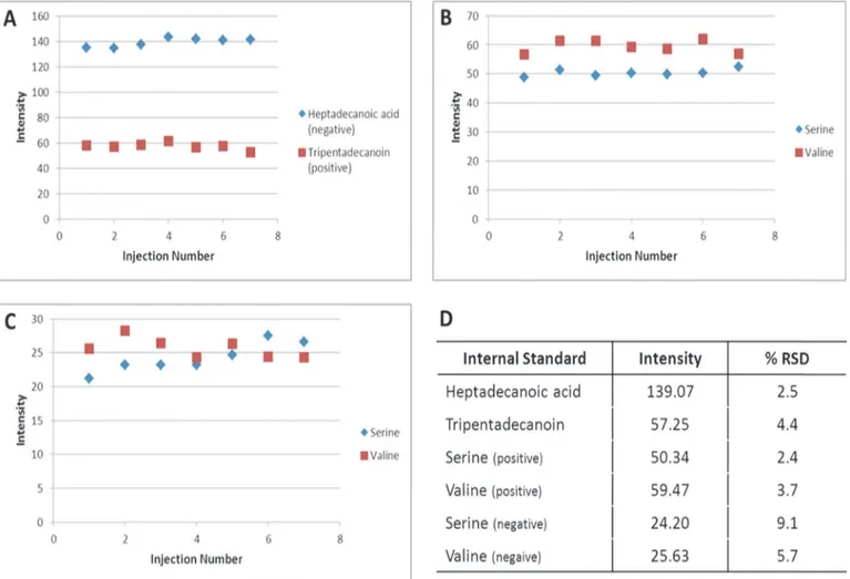
The first step in assessing the precision of the in-vial dual extraction (IVDE) and both the re-versed phase and HILIC methods was to determine the recovery for four internal standards (Fig 3). In the HILIC method both internal standards were measured in both the positive and negative ionisation modes. In the positive data the recovery of internal standards are highly consistent with coefficient of variation (CV) of 2.4% and 3.7% (Fig 3B) for the serine and valine standards respectively. In the negative mode, recovery is more variable than the positive mode with CV’s of 9.1% and 5.7% (Fig 3C) for serine and valine respectively. In the reversed phase method heptadecanoic acid was measured in the negative mode and tripentsdecanoin was measured in the positive. The recovery of both standards was consistent with CV’s of 2.5% and
Fig 3. Recoveries of HILIC and reversed phase internal standards in experiment 1.A) plot of intensity of reversed phase internal standards
Heptadecanoic acid (negative) and Tripentadecanoin (positive), B) plot of intensity of HILIC internal standards in positive ionisation mode, C) plot of intensity of HILIC internal standards in negative ionisation mode, D) average intensity and coefficient of variance of all internal standards.
4.4% for heptadecanoic acid and tripentadenanoin respectively. The standard recoveries sug-gests that the IVDE and both HILIC and reversed phase methods have good precision with all internal standard measurements having CV’s less than 15% [33], with mass spectrometry in the negative mode adding more variability than the positive mode.
The next step in determining the methods performance was to identify the number of me-tabolite features measured following HILIC and reversed phase separation and to assess the precision of these peaks. This was done by initially identifying the features present in all sam-ples, then identifying those features measured in at least of 85% of samsam-ples, with a minimum cut off of peaks present in at least 70% of samples analysed (Tables1and2). In total 5,841 me-tabolite features were measured in 100% of samples for both the HILIC (3713 meme-tabolite fea-tures) and reversed phase (2128 metabolite feafea-tures) methods. When a 70% sample presence cut off was applied, 12,274 metabolite features were identified with 6,570 and 5,704 metabolite features measured in the HILIC and reversed phase methods respectively. The measured me-tabolite features show good precision with 3,468 of the 5,841 (59.4%) of peaks seen in 100% of samples, and 6,362 of the 12,274 (51.8%) of the peaks measured in at least 70% of samples have CV’s of<15%. In general the features with CV’s of15% are lower in abundance, with peaks at CV’s<15% with an average abundance 6.62 and peaks with CV’s15% having an average of 1.93 potentially accounting for the lower precision. It is also interesting to note that the
Table 1. Measured metabolite features in the HILIC method in experiment 1.
HILIC Positive HILIC Negative HILIC Total
%RSD 100%a 85%a 70%a 100%a 85%a 70%a 100%a 85%a 70%a
<5b 141 155 170 103 113 127 244 268 297
5–10b 416 507 598 605 668 726 1021 1175 1324
10–15b 305 436 582 460 618 726 765 1054 1308
15–30b 417 635 889 803 1204 1539 1220 1839 2428
>30b 149 286 406 314 540 807 463 826 1213
Total 1428 2019 2646 2285 3143 3925 3713 5162 6570
Showing the number of metabolite peaks identified and their relative variability in 100%, 85% and 70% of 7 sample replicates.
apercentage of samples a peak is detected in
bcoefficient of variance of peak intensity between samples.
doi:10.1371/journal.pone.0122883.t001
Table 2. Measured metabolite features in the reversed phase method in experiment 1.
RP Positive RP Negative RP Total
%RSD 100%a 85%a 70%a 100%a 85%a 70%a 100%a 85%a 70%a
<5b 124 261 278 202 253 455 326 514 733
5–10b 193 418 450 504 628 1112 697 1046 1562
10–15b 69 115 197 346 418 941 415 533 1138
15–30b 112 246 329 402 484 1009 514 730 1338
>30b 50 134 226 126 340 707 176 474 933
Total 548 1174 1480 1580 2123 4224 2128 3297 5704
Showing the number of metabolite peaks identified and their relative variability in 100%, 85% and 70% of 7 sample replicates.
apercentage of samples a peak is detected in bcoef
ficient of variance of peak intensity between samples.
metabolite features that are measured in all samples have a higher average abundance (4.76) than those measured in 85% (2.04) and 70% (1.83). This is due to these groups possessing more peaks that are close to the limit of detection (LOD) with the peak falling below the LOD in some samples accounting for the missing values.
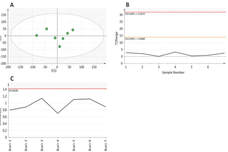
Having considered the behaviour of individual metabolite peaks, the final step in assessing the method performance is to look at the similarity of the overall composition of the analysed samples. Principal component analysis (PCA) was performed on all 12,274 metabolite features that were identified in at least 70% of samples (Fig 4). This PCA revealed little structure within the data with the first component accounting for only 25.3% of the total variability with a pre-dictive performance of Q2= -0.10, with the first two components accounting for just 43.9% of variability with a predictive performance of Q2= -0.21. The distance of a samples metabolite composition to a calculated average composition was assessed using the Hotelling’s T2range plot (Fig 4B). This plot shows that all of the samples are compositionally similar both to each other and the calculated average, with all samples having a T2of<5 with the 95% confidence
interval set at 13.88. The distance of samples to the model was assessed using the DModX plot (Fig 4C), which shows that the samples have a low residual of difference to the fitted model with all of the observations falling below the Dcritical(0.05) threshold. This combined with the Hotelling’s T2show that all of the samples are compositionally similar and that there are no outliers to the model.
Fig 4. Principal component analysis (components = 2, R2X
–0.439, Q2–0.210) of metabolite features identified in at least 70% of samples in
experiment 1.A) scores plot and B) Hotelling’s T2and C) DModX plot, showing that sample mass has no effect on overall metabolite composition.
Assessing the effect of tissue homogenisation and sample mass on
method performance and precision (Experiment 2)
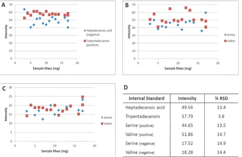
As with assessing the performance of the IVDE and instrument methods, the first step in as-sessing the effect of tissue homogenisation and sample mass is to look at the recovery of the in-ternal standards. As in experiment 1 both HILIC inin-ternal standards are seen in positive and negative ionisation modes (Fig 5B and 5C). In the positive mode the CV’s of the internal stan-dard recoveries were 13.5% and 14.7% for serine and valine respectively. In the negative mode CV’s of the internal standard recoveries were 14.9% and 14.4% for serine and valine respective-ly. In the reversed phase data heptadecanoic acid is measured in the negative mode with a CV of 13.4%, and tripentadecanoin was measured in the positive mode with a CV of 3.8%. The re-covery of the HILIC internal standards is more variable in these samples than in experiment 1, suggesting that the tissue homogenisation step is contributing significantly to analytical vari-ability. This is further supported by no increase in the variability of tripentadecanoin which is spiked into the sample after tissue homogenisation. The recovery of the HILIC internal stan-dards in the quality control samples, which are pooled after tissue homogenisation, were more consistent than in the analytical samples, and comparable with experiment 1 with CV’s of 3.8% and 4.8% in positive and 5.3% and 7.1% in negative for serine and valine respectively, further
Fig 5. Recoveries of HILIC and reversed phase internal standards in experiment 2.A) plot of intensity of reversed phase internal standards
Heptsdecanoic acid (negative) and Tripentadecanoin (positive), B) plot of intensity of HILIC internal standards in positive ionisation mode, C) plot of intensity of HILIC internal standards in negative ionisation mode, D) average intensity and coefficient of variance of all internal standards.
supporting the hypothesis that tissue homogenisation is contributing significantly to the ob-served variability. With the increased CV’s showing that tissue homogenisation is contributing to an increase in data variability, it is important to assess the effect of the extracted tissue vol-ume on the recovery of the internal standards. Spearman’s correlation was used to assess the re-lationship between standard recovery and sample mass, this analysis revealed no significant correlations showing that internal standard recovery is independent of the sample mass extracted.
The next step in assessing the method performance is to determine the number of metabo-lite features measured and the precision of these peaks. As in experiment 1 this was initially done by identifying peaks that were measured in all samples, working down to a cut off of peaks present in at least 73% of samples. In total 4,021 peaks were measured in 100% of sam-ples, with 2,838 and 1,183 measured in HILIC (Table 3) and reversed phase (Table 4) methods respectively, 10,934 peaks measured in 73% of samples with 6,737 and 4,197 measured in HILIC and reversed phase data respectively. The precision of the measured peaks is lower than was seen in experiment 1 with 1,726 of 4,021 (43.7%) of the peaks seen in 100% of samples and 3,151 of 10,934 (28.8%) of peaks seen in 70% of samples having CV’s of<15%. The finding of
higher sample to sample variability of the measured metabolite features lends further support to the hypothesis of tissue homogenisation as a source of variability within the method. A transformation of the HILIC data to correct for the variability introduced during tissue
Table 3. Measured metabolite features in the HILIC method in experiment 2.
HILIC Positive HILIC Negative HILIC Total
%RSD 100%a 93%a 87%a 80%a 73%a 100%a 93%a 87%a 80%a 73%a 100%a 93%a 87%a 80%a 73%a
<5b 38 49 56 68 81 33 39 44 55 61 71 88 100 123 142
5–10b 322 408 431 467 509 217 302 283 344 372 539 710 714 811 881
10–15b 426 566 601 644 685 222 353 386 495 566 648 919 987 1139 1251
15–30b 406 583 742 793 884 501 751 1115 1142 1348 907 1334 1857 1935 2232
>30b 454 610 827 1078 1254 219 362 514 735 977 673 972 1341 1813 2231
Total 1646 2216 2657 3050 3413 1192 1807 2342 2771 3324 2838 4023 4999 5821 6737
Showing the number of metabolite peaks identified and their relative variability in 100%, 93%, 87%, 80% and 73% of 15 sample replicates.
apercentage of samples a peak is detected in
bcoefficient of variance of peak intensity between samples.
doi:10.1371/journal.pone.0122883.t003
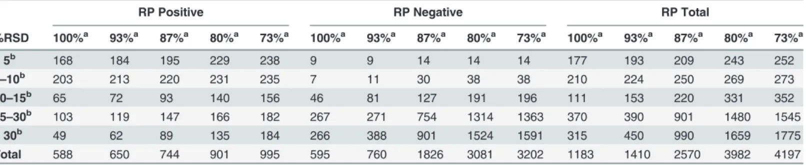
Table 4. Measured metabolite features in the reversed phase method in experiment 2.
RP Positive RP Negative RP Total
%RSD 100%a 93%a 87%a 80%a 73%a 100%a 93%a 87%a 80%a 73%a 100%a 93%a 87%a 80%a 73%a
<5b 168 184 195 229 238 9 9 14 14 14 177 193 209 243 252
5–10b 203 213 220 231 235 7 11 30 38 38 210 224 250 269 273
10–15b 65 72 93 140 156 46 81 127 191 196 111 153 220 331 352
15–30b 103 119 147 166 182 267 271 754 1314 1363 370 390 901 1480 1545
>30b 49 62 89 135 184 266 388 901 1524 1591 315 450 990 1659 1775
Total 588 650 744 901 995 595 760 1826 3081 3202 1183 1410 2570 3982 4197
Showing the number of metabolite peaks identified and their relative variability in 100%, 93%, 87%, 80% and 73% of 15 sample replicates.
apercentage of samples a peak is detected in bcoef
ficient of variance of peak intensity between samples.
homogenisation was performed by normalising peak intensity to an average of the abundance of the two internal standards, however this correction did not improve precision of the mea-sured metabolite peaks (S1 Table).
Having considered metabolite features individually it is important to consider the composi-tion of samples as a whole. As in experiment 1 PCA was applied to all metabolite features that were measured in at least 73% of samples (Fig 6). The analysis revealed little structure within the data with the first component accounting for only 22.3% of total variability with a poor pre-dictive performance of Q2= 0.07, with the second component only explaining a further 13.1% of variability (Q2= 0.05) (Fig 6A). The Hotelling’s T2plot (Fig 6B) shows that all samples fall within the 95% confidence interval (T2= 8.19), with all bar one sample having a T2<4
demon-strating that the samples are compositionally similar both to each other and to the calculated average. The DModX plot (Fig 6C) shows that all samples have a low residual of difference to the fitted model with all of the observations falling below the Dcritical(0.05) threshold. This combined with the Hotelling’s T2plot show that all samples are compositionally similar and that there are no outliers to the model.
Whilst all samples are compositionally similar it is important to determine the effect of the extracted tissue mass on metabolite composition. Looking at the PCA scores plot (Fig 6A) it
Fig 6. Principal component analysis of samples (components = 2, R2X 0.354, Q20.049) performed on metabolite features identified in at least 73% of samples in experiment 2.A) scores plot where point labels represent sample mass B) Hotelling’s T2and C) DModX plot of analytical samples, showing that sample mass has no effect on overall metabolite composition.
can be seen that there is no bias in the distribution of samples based on the tissue mass, with low and high mass samples clustering together within the plot showing that they possess high levels of compositional similarity. As well as looking at the effect of sample mass on the compo-sitional similarity it is important to assess its effect on the abundance of individual metabolites.
Fig 7shows the abundance of 9 annotated metabolites from both HILIC and reversed phase methods plotted against the tissue mass, these plots show no relationship between metabolite abundance and sample mass, with the strongest correlation being for glutamate (r = -0.24). This data shows that using between 3–17mg of sample material has no effect on the overall sample composition or the abundance of individual metabolites, showing this method can pro-vide broad metabolite coverage when sample material is limited.
Annotated metabolites
Having optimised the sensitivity and reproducibility of the metabolite features measured by the analytical method, the final step is to demonstrate its biological relevance by linking the data directly to metabolism by annotating metabolites from a variety of chemical classes and across a range of concentrations. To do these 200 metabolites, 100 from both the HILIC and re-versed phase methods were annotated (Tables5and6). The annotated metabolites come from
Fig 7. Plots of sample mass in milligrams against intensity for 9 annotated metabolites.A) taurine B) hypoxanthine C) glutamate D) pantothenate E) aspartate F) glcosylceramide (36:1) G) phosphatidylethanolamine (38:4) H) ceramide (38:1) I) triglyceride (48:3).
Table 5. Metabolites annotated from the HILIC method.
Name Formula Molecular Weight (Da) Retention time (Mins) Intensity
Positive Negative
Acetylalanine C5H9NO3 131.0582 15.56 6.2
-Acetylaspartate C6H9NO5 175.0480 7.66 6.4 56.2
Acetylaspartylglutamate C11H16N2O8 304.0906 8.38 7.2 28.6
Acetylcarnitine C9H17NO4 203.1157 14.08 27.0 0.4
Acetylneuraminate C11H19NO9 309.1059 23.88 0.4
-Acetylserine C5H9NO4 147.0531 8.31 - 22.3
Adenosine C10H13N5O4 267.0967 12.92 33.3
-Adenosine monophosphate C10H14N5O7P 347.0630 15.60 6.2
-Adrenaline C9H13NO3 183.0895 6.74 2.9
-Alanine C3H7NO2 89.0476 16.61 184.5 39.2
Aminobutyrate C4H9NO2 103.0633 16.25 - 84.5
Arachidonoyl glycidol C23H36O3 360.2664 5.01 7.8
-Arginine C6H14N4O2 174.1116 26.47 40.9 7.4
Ascorbate C6H8O6 176.0320 10.72 4.2 69.1
Asparagine C4H8N2O3 132.0534 17.01 - 1.4
Aspartate C4H7NO4 133.0375 7.81 109.2 33.6
Butyrlcarnitine C11H21NO4 231.1470 12.11 1.7
-Carnitine C7H15NO3 161.1051 17.06 135.5
-Carnosine C9H14N4O3 226.1065 28.8 2.1
-Citrate C6H8O7 192.0270 10.7 - 1.2
Citrulline C6H13N3O3 175.0956 17.17 2.7 2.2
Coumarate C9H8O3 164.0473 14.40 26.7
-Creatine C4H9N3O2 131.0694 16.62 576.9 20.5
Creatinine C4H7N3O 113.0589 16.61 15.6 1.0
Cystathionine C7H14N2O4S 222.0674 21.74 7.4 1.2
Cysteine C3H7NO2S 121.0197 15.30 2.8
-Cytidine C9H13N3O5 243.0855 17.33 2.1 1.2
Deoxyfluorouridine C9H11FN2O5 246.0651 12.20 - 6.2
Dimethylarginine C8H18N4O2 202.1429 24.45 1.4
-Dimethylglycine C4H9NO2 103.0633 17.21 24.9
-Fumarate C4H4O4 116.0109 7.78 - 0.8
Gluconate C6H12O7 196.0583 15.64 - 43.1
Glutamate C5H9NO4 147.0531 16.17 79.1 61.6
Glutamine C5H10N2O3 146.0691 16.78 27.9 95.2
Glutamyl-glutamate C10H14N2O7 274.0801 15.61 8.2
-Glutamyl-leucine C11H19N2O5 259.1293 15.48 2.8
-Glutathione C10H17N3O6S 307.0838 15.06 22.8
-Glycerophosphatidylcholine C8H20NO6P 257.1028 18.06 42.4
-Glycine C2H5NO2 75.0320 17.13 2.2 1.3
Glycolate C2H4O3 76.0160 6.51 - 4.5
Guanidinobutanoate C5H11N3O2 145.0851 15.73 8.4
-Guanine C5H5N5O 151.0494 11.90 13.5 7.9
Guanosine C10H13N5O5 283.0916 11.87 2.3 18.4
Hexose-deoxy sugar C6H12O5 164.0679 14.39 - 5.2
Hexose-Phosphate C6H13O9P 260.0297 14.94 - 17.4
Histidine C6H9N3O2 155.0694 25.13 14.6 6.1
Hydroxyphenylglycine C8H9NO3 167.0582 16.61 - 0.7
Hydroxyproline C5H9NO3 131.0582 16.17 - 1.6
Hypoxanthine C5H4N4O 136.0385 9.45 489.9 108.7
Indoleacetate C10H9NO2 175.0633 9.17 5.0
-Inosine C10H12N4O5 268.0807 10.03 45.7 388.8
Kynurenine C10H12N2O3 208.0847 12.19 0.9
-Lactate C3H6O3 90.0316 7.57 - 6.1
leucine/Isoleucine C6H13NO2 131.0946 12.69 20.3 1.6
Lysine C6H14N2O2 146.1055 26.62 4.7 16.3
Table 5. (Continued)
Name Formula Molecular Weight (Da) Retention time (Mins) Intensity
Positive Negative
Lysophosphatidylserine C24H48NO9P 326.3033 6.89 4.9
-Malate C4H6O5 134.0215 8.66 - 9.5
Malonate C3H4O4 104.0109 7.27 0.4
-Methionine C5H11NO2S 149.0510 13.43 7.3 1.2
Methyladenosine C11H15N5O4 281.1124 17.16 0.9 0.7
Methylaspartate C5H9NO4 147.0531 8.39 48.4 20.3
Methylbutyroylcarnitine C12H23NO4 245.1627 11.8 0.3
-Methylfuranone C6H8O2 98.0368 15.66 - 223.4
Methylhistidine C7H11N3O2 169.0851 25.54 2.2
-Methylsulfolene C5H8O2S 132.0245 13.44 16.9
-Methylthioadenosine C11H15N5O3S 297.0895 10.61 1.3
-Methylthiophene C5H6S 98.0190 7.80 1.2
-Myo-inositol C6H12O6 180.0633 15.83 5.3 5.0
Nicotinamide C6H6N2O 122.0480 9.57 104.8
-Nicotinate C6H5NO2 123.0320 9.14 - 0.6
Ornithine C5H12N2O2 132.0898 26.39 0.5 14.4
Oxoproline C5H7NO3 129.0425 16.77 217.42 30.2
Pantothenate C9H17NO5 219.1106 6.74 10.1 2.2
Pentose sugar C5H10O5 150.0528 13.55 - 10.7
Phenylalanine C9H11NO2 165.0789 12.03 9.2 0.4
Phosphatidylcholine C40H80NO8P 733.5621 9.08 63.6
-Phosphenolpyruvate C3H5O6P 167.9823 12.09 - 0.4
Phosphocreatine C4H10N3O5P 211.0358 15.05 4.1
-Pipecolate C6H11NO2 129.0789 14.76 1.7
-Proline C5H9NO2 115.0633 14.99 30.2 0.3
Propionylcarnitine C10H19NO4 217.1314 12.92 1.3
-Putrescine C4H12N2 88.1000 34.8 - 0.8
Riboflavin C17H20N4O6 376.1382 7.9 5.5
-Serine C3H7NO3 105.0425 17.06 4.2 1.9
Spermidine C7H19N3 145.1578 30.46 1.1
-Taurine C2H7NO3S 125.0146 15.00 119.9 286.3
Thiouracil C4H4N2OS 128.0044 8.4 - 0.9
Threonine/Homoserine C4H9NO3 119.0582 16.37 6.9
-Thymidine C10H14N2O5 242.0902 8.2 - 1.6
Thymine C5H6N2O2 126.0429 9.30 0.6 25.6
Tocopherol C29H50O2 430.3810 20.89 5.1
-Tryptophan C11H12N2O2 204.0898 12.74 4.2 1
Tyrosine C9H11NO3 181.0738 14.39 8.8 14.9
Uracil C4H4N2O2 112.0272 9.14 27.3 6.3
Urate C5H4N4O3 168.0283 11.19 2.3 3.8
Uridine C9H12N2O6 244.0695 9.18 1.7 12.1
Valine C5H11NO2 117.0789 14.66 4.6 0.9
Xanthine C5H4N4O2 152.0334 8.88 78.1 51.7
Xanthosine C10H12N4O6 284.0756 11.85 - 2.8
Xanthurenate C10H7NO4 205.0375 11.20 1.4
-Annotations were made by matching fragmentation of analyte peaks to fragmentations in publicly accessible databases. Displaying the molecular formula, molecular weight in daltons, retention time in minutes and intensity in positive and negative ionisation modes in arbitrary units for all metabolites.— represents metabolites not detected in this ionisation mode.
Table 6. Metabolites annotated from the reversed phase method.
Name Formula Molecular Weight (Da) Retention time (Mins) Intensity
Positive Negative
Docosahexaenoic acid C22H32O2 328.2400 5.02 - 16.8
Hexadecynyl acetate C18H32O2 280.2388 4.61 - 1.7
Hydroxycholestanol C27H48O2 404.3636 15.06 - 3.7
DG(40:5) C43H74O5 670.5536 20.79 1.8
-DG(34:2) C37H68O5 592.5066 27.07 0.7
-DG(42:3) C45H82O5 702.6162 17.58 3.9
-DG(37:2) C40H74O5 634.5536 27.14 1.2
-SM(d34:1) C39H80N2O6P 703.5753 13.20 0.7
-SM(41:2) C46H92N2O6P 799.6693 25.84 4.6
SM(d41:1) C46H94N2O6P 801.6849 18.55 1.9
-SM(d42:1) C47H96N2O6P 815.7006 24.13 3.9
-SM(d43:2) C48H96N2O6P 827.7006 20.20 18.9
-Creatine 16:1 OH C39H77N2O7P 716.5468 16.53 - 10.2
TG(52:7) C55H92O6 848. 6893 28.10 6.2
-TG(52:3) C55H100O6 856.7519 19.44 1.4
-TG(48:3) C51H92O6 800.6823 17.70 2.3
-TG(50:3) C53H96O6 828.7112 19.97 1.1
-TG(54:7) C57H96O6 876.7199 30.36 3.1
-TG(54:6) C57H98O6 878.7420 30.43 1.1
-TG(56:7) C59H98O6 902.7421 32.71 1.2
-PI(34:1) C43H81O13P 836.5414 12.32 73.1
-PI(36:3) C45H81O13P 860.5414 21.29 - 6.93
PI(32:0) C41H79O13P 810.5258 20.97 - 19.00
PI(38:2) C47H87O13P 891.1596 19.08 - 34.13
PI(40:5) C49H85O13P 912.5727 16.31 3.2
PI(38:5) C47H81O13P 884.5414 23.33 7.2
-PA(36:2) C39H73O8P 700.9659 15.97 1.4
-PA(34:1) C37H71O8P 674.9286 20.68 32.8
-PA(39:0) C42H85O7P 732.6091 14.89 0.9
-PA(34:2) C37H69O8P 672.4730 20.33
GluCer(36:1) C42H81NO8 727.5962 24.19 5.2
-GluCer(d40:1) C46H89NO8 783.6588 23.02 16.7
-GluCer(d40:2) C46H87NO8 781.6351 23.60 1.1 4.3
GluCer(42:2) C48H91NO8 809.6744 19.18 1.8
-PC(31:2) C39H74NO8P 715.5134 18.85 2.4
-PC(36:2) C44H84NO7P 770.7432 18.36 1.5
-PC(33:2) C41H78NO8P 743.5492 20.21 1.7 12.1
PC(32:3) C42H74NO8P 751.5152 18.77 - 57.7
PC(33:1) C41H80NO8P 745.5574 21.30 - 0.3
PC(37:6) C45H78NO8P 791.5417 19.61 - 1.9
PC(32:2) C40H76NO8P 729.5322 15.98 13.7
-PC(38:9) C46H74NO8P 799.5298 19.11 - 45.4
PC(35:0) C43H86NO8P 775.6091 15.75 0.71
PC(35:6) C43H74NO8P 763.5146 18.70 2.3 22.4
PC(35:3) C43H80NO8P 769.5688 20.70 41.5
-PC(35:6) C43H74NO8P 763.5146 17.63 2.1
Table 6. (Continued)
Name Formula Molecular Weight (Da) Retention time (Mins) Intensity
Positive Negative
PC(35:3) C43H80NO8P 769.5688 25.57 1.5
-PC(36:3) C44H82NO8P 783.5663 15.49 15.7
-PC(P-38:5) C46H82NO7P 791.5828 14.78 0.5
-PC(44:1) C52H103NO8P 900.7242 24.05 19.9
-PC(P-38:6) C46H80NO7P 789.5609 18.20 1.0
-PC(44:0) C52H105NO8P 902.7421 28.94 18.6
-PC(45:0) C53H107NO8P 916.6589 27.84 11.5
-PC (38:0) C46H92NO8P 817.6561 26.70 3.2
-PC (40:1) C48H94NO8P 843.6717 20.24 6.6 6.4
PC (40:6) C48H84NO8P 833.5935 18.78 1.5 68.1
PC (38:6) C44H76NO8P 805.5622 15.60 16.8
-PC (40:2) C48H92NO8P 841.6560 21.07 - 3.6
PG(34:1) C40H77O10P 748.5254 14.43 3.0
-PG(38:3) C44H81O10P 800.5567 17.50 14.8
-PG(36:2) C42H79O10P 774.5410 17.53 1.4
-PG(42:0) C48H97O9P 848.6842 19.75 2.7
-PE(35:0) C40H80NO8P 733.5621 13.31 1.3
PE(40:6) C45H78NO8P 791.5417 19.61 - 31.3
PE(33:1) C38H74NO8P 703.5158 16.54 24.6
-PE(35:2) C40H80NO8P 729.5308 25.83 4.9
-PE(38:3) C43H80NO8P 769.5688 25.96 24.2
-PE(33:2) C38H72NO8P 701.4996 18.18 36.9
PE(34:2) C39H74NO8P 715.5134 18.85 - 12.4
PE(36:4) C41H76NO8P 739.5154 12.76 0.1
-PE(36:2) C41H78NO8P 743.5492 14.70 2.4
-PE(36:5) C41H72NO8P 737.4995 21.03 2.5
-PE(36:1) C41H76NO8P 745.5574 20.23 - 0.3
PE(38:6) C43H74NO8P 763.5156 18.70 12.2
-PE(38:4) C43H78NO8P 768.0551 23.40 6.4
-PE(46:1) C51H100NO8P 885.7367 22.07 7.6
-PE(O-36:0) C41H86NO6P 719.6105 12.32 0.1
-PE(40:2) C45H86NO8P 799.6091 16.03 1.0
-PE(44:8) C49H82NO8P 844.5151 19.64 3.2
-LPC(18:2) C26H50NO7P 519.3324 12.10 2.8
LPC(20:4) C28H50NO7P 543.3353 11.80 3.1
-LPC(24:1) C32H64NO7P 605.4384 9.13 2.1
-LPA(18:0) C21H43O7P 438.2746 15.97 0.9
LPE(22:0) C27H56NO7P 537.7098 15.76 - 10.1
LPE(24:1) C29H58NO7P 563.7471 16.41 - 7.2
PS(30:1) C36H68NO10P 705.4580 18.33 0.3
-PS(38:3) C44H80NO10P 813.5519 21.55 - 1.9
PS(40:5) C46H80NO10P 837.5519 12.44 0.7
-PS(37:3) C43H78NO10P 799.5298 10.64 - 1.5
PS(36:1) C42H80NO10P 789.5609 13.75 0.8
-PS(36:0) C42H82NO10P 791.5800 14.77 0.4
a wide range of metabolite classes including amino acids, purines, phospholipids and glycer-ides, across 3.5 orders of magnitude ranging in abundance from 0.1 to 576.9. There is limited overlap between the two analytical methods with no identified metabolites in common, this limited overlap demonstrates the necessity of using complimentary separation techniques like HILIC and reversed phase chromatography to obtain a comprehensive view of all of chemical space. These annotations enable the method to be easily compared as basal metabolite abun-dance in the rat’s healthy cerebellum and provide valuable information allowing the method to be accurately replicated by other laboratories.
Conclusions
The method described in this paper is shown to be capable of measuring over 4,000 metabolite features from as little as 3mg of tissue with a high degree of reproducibility of which we were able to annotate 200 metabolites from a variety of metabolite classes across a range of concen-trations. It is hoped that the low required sample mass and improved sensitivity of this method will provide a valuable tool to analyse cerebral metabolism, hopefully providing new insights into the functioning of the brain as well as the mechanisms of pathology of neurological disorders.
Supporting Information
S1 Table. Measured metabolite features in the HILIC method in experiment 2.Showing the number of metabolite peaks identified and their relative variability in 100%, 93%, 87%, 80% and 73% of 15 sample replicates after transformation based on the recovery of both internal standards.apercentage of samples a peak is detected in,bcoefficient of variance of peak inten-sity between samples.
(DOCX)
Table 6. (Continued)
Name Formula Molecular Weight (Da) Retention time (Mins) Intensity
Positive Negative
PS(36:5) C42H72NO10P 781.9955 12.70 1.1
-PS(0–34:0) C40H80NO9P 749.5511 14.55 0.3
-PS(34:1) C40H76O10P 761.5975 16.88 1.3
-Cer(36:1) C36H67NO3 565.5435 17.49 - 8.6
Cer(38:1) C38H67NO3 593.5745 19.16 - 2.7
Cer(40:1) C40H67NO3 621.6163 20.60 - 1.9
Cer(42:1) C42H83NO3 649.6372 20.83 - 1.2
Cer(d44:2) C44H85NO3 675.6477 24.30 5.6
-Cer(d40:1) C40H80NO6P 701.5575 15.13 3.8
-Annotations were made by matching fragmentation of analyte peaks to fragmentations in publicly accessible databases. Displaying the molecular formula, molecular weight in daltons, retention time in minutes and intensity in positive and negative ionisation modes in arbitrary abundance units for all
metabolites.—represents metabolites not detected in this ionisation mode.Abbreviations:Lysophosphatidylcholines (LPC),
Lysophosphatidylethanolamines (LPE),Phosphatidic acids (PA), Phosphatidylcholines (PC), Ether-linked phosphatidylethanolamines (PE-O), Phosphatidylglycerols (PG), Phosphatidylinositols (PI), Phosphatidylserines (PS), Ether-linked phosphatidylserines(PS-O), Ether-linked phosphatidylserines (PS-O), Sphingomyelins (SM), Dihydroxy-glucosylceramide (GluCer-d), Dihydroxyceramide (Cer-d), Triacylglycerols (TG), Diacylglycerols (DG).
Acknowledgments
This work has been supported by grants from the Butterfield Trust and the Libyan Cultural at-taché of Libyan embassy. We would also like to thank Dr Chantal Bazenet for critically reading the manuscript and providing constructive feedback, Dr Mathew Arno manager of the geno-mics centre for permitting us to use his Tissuelyzer and Juzaili Azizi for aiding us with rat brain dissection.
Author Contributions
Conceived and designed the experiments: CLQ. Performed the experiments: AAE SGS. Ana-lyzed the data: AAE SGS. Contributed reagents/materials/analysis tools: CLQ. Wrote the paper: AAE SGS MT RP AH CLQ.
References
1. Available:http://www.nlm.nih.gov/medlineplus/neurologicdiseases.html.
2. Rice ML, Warren SF, Betz SK. (May 2005). "Language symptoms of developmental language disor-ders: An overview of autism, Down syndrome, fragile X, specific language impairment, and Williams syndrome." Applied Psycholinguistics, 26:1. pp. 7–27.
3. Geschwind DH, Levitt P (2007) Autism spectrum disorders: developmental disconnection syndromes. Current Opinion in Neurobiology 17, 103–111. PMID:17275283
4. Niedermeyer E, Froescher W, Fisher RS (1985) Epileptic seizure disorders. Journal of Neurology 232, 1–12. PMID:3998776
5. Jankovic J (2008) Parkinson's disease: clinical features and diagnosis. Journal of Neurology, Neurosur-gery & Psychiatry 79, 368–376.
6. McKhann G, Drachman D, Folstein M, Katzman R, Price D, Stadlan EM, et al. (1984) Clinical diagnosis of Alzheimer's disease: Report of the NINCDS-ADRDA Work Group*under the auspices of Depart-ment of Health and Human Services Task Force on Alzheimer's Disease. Neurology 34, 939.
7. Proitsi P, Kim M, Whiley L, Pritchard M, Leung R, Soininen H, et al. (2015) Plasma lipidomics analysis finds long chain cholesteryl esters to be associated with Alzheimer/'s disease. Transl Psychiatry 5, e494. doi:10.1038/tp.2014.127PMID:25585166
8. Whiley L, Sen A, Heaton J, Proitsi P, García-Gómez D, Leung R, et al. (2014) Evidence of altered phos-phatidylcholine metabolism in Alzheimer's disease. Neurobiology of Aging 35, 271–278. doi:10.1016/j. neurobiolaging.2013.08.001PMID:24041970
9. Snowden S, Dahlan S-E, Wheelock CE (2012) Application of metabolomics approaches to the study of respiratory diseases. Bioanalysis 4, 2265–2290. doi:10.4155/bio.12.218PMID:23046268
10. Fiehn O (2002) Metabolomics—the link between genotypes and phenotypes. Plant Molecular Biology 48, 155–171. PMID:11860207
11. Psychogios N, Hau DD, Peng J, Guo AC, Mandal R, Bouatra S, et al. (2011) The Human Serum Meta-bolome. PLoS ONE 6, e16957. doi:10.1371/journal.pone.0016957PMID:21359215
12. Pan Z, Raftery D (2007) Comparing and combining NMR spectroscopy and mass spectrometry in metabolomics. Analytical and Bioanalytical Chemistry 387, 525–527. PMID:16955259
13. Zhang T, Creek DJ, Barrett MP, Blackburn G, Watson DG (2012) Evaluation of Coupling Reversed Phase, Aqueous Normal Phase, and Hydrophilic Interaction Liquid Chromatography with Orbitrap Mass Spectrometry for Metabolomic Studies of Human Urine. Analytical Chemistry 84, 1994–2001.
14. Kell DB (2004) Metabolomics and systems biology: making sense of the soup. Current Opinion in Mi-crobiology 7, 296–307. PMID:15196499
15. Crockford DJ, Holmes E, Lindon JC, Plumb RS, Zirah S, Bruce SJ, et al. (2005) Statistical Heterospec-troscopy, an Approach to the Integrated Analysis of NMR and UPLC-MS Data Sets: Application in Metabonomic Toxicology Studies. Analytical Chemistry 78, 363–371.
16. Kleijn RJ, Geertman J-MA, Nfor BK, Ras C, Schipper D, Pronk JT, et al. (2007) Metabolic flux analysis of a glycerol-overproducing Saccharomyces cerevisiae strain based on GC-MS, LC-MS and NMR-de-rived 13C-labelling data. FEMS Yeast Research 7, 216–231. PMID:17132142
18. Llorach R, Urpi-Sarda M, Jauregui O, Monagas M, Andres-Lacueva C (2009) An LC-MS-Based Meta-bolomics Approach for Exploring Urinary Metabolome Modifications after Cocoa Consumption. Journal of Proteome Research 8, 5060–5068. doi:10.1021/pr900470aPMID:19754154
19. De Vos RCH, Moco S, Lommen A, Keurentjes JJB, Bino RJ, Hall RD (2007) Untargeted large-scale plant metabolomics using liquid chromatography coupled to mass spectrometry. Nat. Protocols 2, 778–791. PMID:17446877
20. Lanza IR, Zhang S, Ward LE, Karakelides H, Raftery D, Nair KS (2010) Quantitative Metabolomics by 1H-NMR and LC-MS/MS Confirms Altered Metabolic Pathways in Diabetes. PLoS ONE 5, e10538. doi:10.1371/journal.pone.0010538PMID:20479934
21. Mallet CR, Lu Z, Mazzeo JR (2004) A study of ion suppression effects in electrospray ionization from mobile phase additives and solid-phase extracts. Rapid Communications in Mass Spectrometry 18, 49–58. PMID:14689559
22. Annesley TM (2003) Ion Suppression in Mass Spectrometry. Clinical Chemistry 49, 1041–1044. PMID: 12816898
23. Muller C, Schafer P, Stortzel M, Vogt S, Weinmann W (2002) Ion suppression effects in liquid chroma-tography electrospray-ionisation transport-region collision induced dissociation mass spectrometry with different serum extraction methods for systematic toxicological analysis with mass spectra librar-ies. Journal of Chromatography B 773, 47–52. PMID:12015269
24. Antignac J-P, de Wasch K, Monteau F, De Brabander H, Andre F, Le Bizec B (2005) The ion suppres-sion phenomenon in liquid chromatography-mass spectrometry and its consequences in the field of residue analysis. Analytica Chimica Acta 529, 129–136.
25. Michopoulos F, Lai L, Gika H, Theodoridis G, Wilson I (2009) UPLC-MS-Based Analysis of Human Plasma for Metabonomics Using Solvent Precipitation or Solid Phase Extraction. Journal of Proteome Research 8, 2114–2121. PMID:19714883
26. Dunn WB, Broadhurst DI, Atherton HJ, Goodacre R, Griffin JL (2011) Systems level studies of mamma-lian metabolomes: the roles of mass spectrometry and nuclear magnetic resonance spectroscopy. Chemical Society Reviews 40, 387–426. doi:10.1039/b906712bPMID:20717559
27. Wishart DS (2011) Advances in metabolite identification. Bioanalysis 3, 1769–1782. doi:10.4155/bio. 11.155PMID:21827274
28. Salek RM, Xia J, Innes A, Sweatman BC, Adalbert R, Randle S, et al. (2010) A metabolomic study of the CRND8 transgenic mouse model of Alzheimer's disease. Neurochemistry International 56, 937– 947. doi:10.1016/j.neuint.2010.04.001PMID:20398713
29. Graham SF, Chevallier OP, Roberts D, Halscher C, Elliott CT, Green BD (2013) Investigation of the Human Brain Metabolome to Identify Potential Markers for Early Diagnosis and Therapeutic Targets of Alzheimer's Disease. Analytical Chemistry 85, 1803–1811. doi:10.1021/ac303163fPMID:23252551
30. Inoue K, Tsutsui H, Akatsu H, Hashizume Y, Matsukawa N, Yamamoto T, et al. (2013) Metabolic profil-ing of Alzheimer's disease brains. Sci. Rep. 3.
31. Spijker S (2011) Dissection of Rodent Brain Regions In Neuroproteomics Humana Press, pp. 13–26.
32. Whiley L, Godzien J, Ruperez FJ, Legido-Quigley C, Barbas C (2012) In-Vial Dual Extraction for Direct LC-MS Analysis of Plasma for Comprehensive and Highly Reproducible Metabolic Fingerprinting. Ana-lytical Chemistry 84, 5992–5999. doi:10.1021/ac300716uPMID:22702345