Technical Note: Simple formulations and solutions of the dual-phase diffusive transport for biogeochemical modeling

(1)

BGD

11, 1587–1611, 2014

Simple formulations and solutions of the dual-phase diffusive

transport

J. Y. Tang and W. J. Riley

Title Page

Abstract Introduction

Conclusions References

Tables Figures

◭ ◮

Back Close

Full Screen / Esc

Printer-friendly Version Interactive Discussion

Discussion

P

a

per

|

D

iscussion

P

a

per

|

Discussion

P

a

per

|

Discuss

ion

P

a

per

|

Biogeosciences Discuss., 11, 1587–1611, 2014 www.biogeosciences-discuss.net/11/1587/2014/ doi:10.5194/bgd-11-1587-2014

Open Access

Biogeosciences

Discussions

This discussion paper is/has been under review for the journal Biogeosciences (BG). Please refer to the corresponding final paper in BG if available.

Technical Note: Simple formulations and

solutions of the dual-phase di

_ff

usive

transport for biogeochemical modeling

J. Y. Tang and W. J. Riley

Department of Climate and Carbon Sciences, Earth Sciences Division, Lawrence Berkeley National Lab (LBL), Berkeley, CA, USA

Received: 12 January 2014 – Accepted: 15 January 2014 – Published: 23 January 2014

Correspondence to: J. Y. Tang (jinyuntang@lbl.gov)

(2)

BGD

11, 1587–1611, 2014

transport

Title Page

Tables Figures

◭ ◮

Back Close

Full Screen / Esc

Discussion

P

a

per

|

D

iscussion

P

a

per

|

Discussion

P

a

per

|

Discuss

ion

P

a

per

|

Abstract

Representation of gaseous diffusion in variably saturated near-surface soils is becom-ing more common in land biogeochemical models, yet the formulations and numerical solution algorithms applied vary widely. We present three di_fferent but equivalent for-mulations of the dual-phase (gaseous and aqueous) tracer diffusion transport problem

5

that is relevant to a wide class of volatile tracers in land biogeochemical models. Of these three formulations (i.e., the gas-primary, aqueous-primary, and bulk tracer based formulations), we contend the gas-primary formulation is the most convenient for mod-eling tracer dynamics in biogeochemical models. We then provide finite volume approx-imation to the gas-primary equation and evaluate its accuracy against three analytical

10

models: one for steady-state soil CO2dynamics, one for steady-state soil CO2

dynam-ics, and one for transient tracer diffusion from a constant point source into two different sequentially aligned medias. All evaluations demonstrated good accuracy of the nu-merical approximation. We expect our result will standardize an efficient mechanistic numerical method for solving relatively simple, multi-phase, one-dimensional diffusion

15

problems in land models.

1 Introduction

The interest in predicting fluxes of various biogenic greenhouse gases and their in-teractions with climate change has motivated the development of many terrestrial bio-geochemical models; e.g., ecosystem methane models (Walter and Heiman, 2000;

20

Zhuang et al., 2004; Tang et al., 2010; Riley et al., 2011), nitrification-denitrification models (Venterea and Rolston, 2000; Maggi et al., 2008), water-CO₂ isotope models (Riley et al., 2002), and generic reactive transport models that attempt to integrate as many biogeochemical processes and chemical species as possible (e.g., Simunek and Suarez, 1993; Grant, 2001; Tang et al., 2013). To resolve the depth-dependent

dy-25

(3)

BGD

11, 1587–1611, 2014

transport

Title Page

Tables Figures

◭ ◮

Back Close

Full Screen / Esc

Discussion

P

a

per

|

D

iscussion

P

a

per

|

Discussion

P

a

per

|

Discuss

ion

P

a

per

|

namics, these models in general represent multiphase (aqueous and gaseous phase) diffusion processes and often assume negligible advection.

The equation for multiphase diffusion has been represented in different forms by dif-ferent authors (Table 1). However, the numerical implementation of the equation is often vaguely described (either by referring to other publications or by mentioning the

numer-5

ical scheme) or is convolved with other technical details, making the model difficult to understand or replicate by other researchers. In many cases, however, one does not need to represent all the processes typically included in a complicated reactive trans-port model to understand a particular problem. For instance, when soil moisture and temperature data are available together with soil respiration, one only needs a diff

u-10

sion model to evaluate belowground CO₂dynamics (Davidson et al., 2006). Therefore, ecosystem models would benefit from a simple mechanistic formulation and numerical implementation of the dual-phase diffusion problem.

In this note, we categorize the existing formulations of the dual-phase di_ffusion prob-lem into three forms, and recommend one that can be most easily impprob-lemented

numer-15

ically in land models. We hope that this effort will help researchers who wish to develop simple but mechanistic transport models for their particular problem.

2 Methods

2.1 Governing equations

In this section we derive the relevant mass balance differential equations from first

20

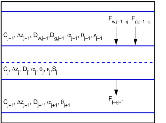
principles. Throughout this note we assume advection is treated using the operator splitting method (Tang et al., 2013), or is negligible. Considering the diffusive mass transport problem (Fig. 1), the dual-phase diffusive flux from layerj−1 intoj is

(4)

BGD

11, 1587–1611, 2014

transport

Title Page

Tables Figures

◭ ◮

Back Close

Full Screen / Esc

Discussion

P

a

per

|

D

iscussion

P

a

per

|

Discussion

P

a

per

|

Discuss

ion

P

a

per

|

Fw,j−1→j =−

θDw ∂Cw

∂z

j−1

2

(1b)

Fg,j−1→j =− εDg ∂Cg

∂z

!

j−1

2

(1c)

where subscript w indicates aqueous diffusion and subscript g indicates gaseous diff u-sion. Soil moisture is represented byθand air-filled porosity by ε. The fluxes (Fj−1→j)

5

are imposed at the upper and lower boundaries of layerj. Tracer concentrations are designated byCwith appropriate subscripts. In defining the effective aqueous (Dw) and

gaseous (Dg) diffusivities, we assume the tortuosity has been considered appropriately

(e.g., Moldrup et al., 2003). A full list of symbols is given in Table A1. Applying the law of mass balance to layerj

10

∆z_j∆Cj

∆t =Fj−1→j−Fj→j+1= Fw,j−1→j−Fw,j→j+1

+ Fg,j−1→j−Fg,j→j+1

+S_j∆z_j (2a)

and in the limit of small∆zj and∆t, one obtains

∂C

∂t =

∂ ∂z

θDw ∂Cw

∂z

+ ∂

∂z εDg

∂Cg ∂z

!

+S(C,z) (2b)

where S(C,z) is the tracer source due to processes other than diffusion and C is the bulk tracer concentration including both gaseous and aqueous phases. From the

15

assumption of equilibrium between aqueous and gaseous phases (e.g., Tang et al., 2010):

C=θCw+εCg=RgCg=(θα+ε)Cg=RwCw=

θ+_αεCw (3)

(5)

BGD

11, 1587–1611, 2014

transport

Title Page Abstract Introduction Conclusions References Tables Figures ◭ ◮ ◭ ◮ Back Close

Full Screen / Esc

Printer-friendly Version Interactive Discussion Discussion P a per | D iscussion P a per | Discussion P a per | Discuss ion P a per |

whereα is the Bunsen solubility coefficient, one obtains, from substitution of Eq. (3) into the diffusion and temporal derivative of Eq. (2b):

Rg ∂Cg ∂t = ∂ ∂z "

αθDw+εDg

∂Cg

∂z

#

+S(C,z) (4a)

Rw ∂Cw ∂t = ∂ ∂z

θDw+ ε αDg

∂C_w

∂z

+S(C,z) (4b)

5

By further defining a bulk di_ffusivity

D=αθDw+εDg

Rg

=θDw+εDg/α

Rw (5) and assuming 1 Cx ∂C_x ∂t ≫ 1 Rx ∂R_x ∂t , 1 Cx ∂C_x ∂z ≫ 1 Rx ∂R_x ∂z

, x=w or g (6)

one finds for the bulk tracer:

10 ∂C ∂t = ∂ ∂z D∂C ∂z

+S(C,z) (7)

Clearly, Eqs. (4a) (gas-primary form), (4b) (aqueous-primary form), and (7) (bulk tracer form) are equivalent, but Eq. (4) are more convenient to solve because the tracer sources are in general given as aqueous reactions or gaseous sinks (e.g., plant transport, ebullition) and the necessary phase conversion can be done easily through

15

Eq. (3). In particular, Eq. (4a) (the gas-primary form) is the most convenient for sim-ulating volatile tracers and can be applied to variably saturated soil without the need for special care of the air–water interface, as was done in a few existing wetland-CH4

models (see remark in Table 1). We note that Eq. (4a) was also used by Simunek and Suarez (1993) to model CO₂transport in soil.

(6)

BGD

11, 1587–1611, 2014

transport

Title Page

Tables Figures

◭ ◮

Back Close

Full Screen / Esc

Discussion

P

a

per

|

D

iscussion

P

a

per

|

Discussion

P

a

per

|

Discuss

ion

P

a

per

|

At the top boundary, conditions are in general given as gas tracer concentrations, which are connected to the gas concentration of the top numerical layer as

Fg,0→1=−

Cg,1−Ca ra+rs

(8)

wherer_ais atmospheric resistance andr_s is soil resistance (see Tang and Riley, 2013, for a detailed discussion).

5

At the bottom boundary, zero flux conditions are often imposed, though zero concen-tration can also be used for particular problems. In practice, if a tracer exists only in the aqueous phase, then one can solve Eq. (4b) for aqueous di_ffusive transport by setting

α→ ∞and using a zero-flux boundary condition at the top and bottom boundaries.

2.2 Numerical implementation

10

We now solve Eq. (4a) using the finite volume method. First, we discretize the equation spatially and convert it into the following ordinary differential equation (ODE) system,

diag Z_gd

C_g

dt =ACg+S (9a)

where diag (V_{) indicates a diagonal matrix formed by the vector}V _and

C₌

Cg,1· · ·Cg,j · · ·Cg,N T

(9b)

15

A=



      

−c₁_/₂−c₃_/₂ c₃_/₂ 0 · · · 0

..

. ... ... · · · 0

· · · c_j−1/2−cj−1/2−cj+1/2 cj+1/2 · · ·

..

. 0 · · · ...

0 · · · 0 c_N−1/2−cN−1/2−cN+1/2



      

(9c)

S₌_S₍_C₁_,_z₁₎_∆_z₁₊_c₁_/₂_C_a· · ·S C_j,z_j∆z_j · · ·S(C_N,z_N)∆z_N+c_N₊₁_/₂C_bT (9d)

(7)

BGD

11, 1587–1611, 2014

transport

Title Page

Tables Figures

◭ ◮

Back Close

Full Screen / Esc

Discussion

P

a

per

|

D

iscussion

P

a

per

|

Discussion

P

a

per

|

Discuss

ion

P

a

per

|

Z_g₌

Rg,1∆z1· · ·Rg,j∆zj · · ·Rg,N∆zN (9e)

Other coefficients are defined as

Dwg,j =αjθjDw,j+εjDg,j, 1< j≤N (10a)

cj−1/2=

∆z_j−1

2Dwg,j−1

+ ∆zj 2Dwg,j

!−1

, 1< j≤N (10b)

5

c1/2=

1

ra+rs

(10c)

Conductance c_N₊1/2 is zero when zero flux bottom boundary condition is used, but

here it is included to enable Eq. (9) to accommodate the bottom boundary condition given as a constant tracer concentration (Cb). For this latter case, one can simply set

10

c_N₊1/2tocN−1/2.

The ODE system formed by Eq. (9) (together with Eq. 10) can be easily solved with various temporal discretization methods. For instance, the ODE solvers (e.g., ODE45, ODE23) in MATLAB provide a very straightforward way to obtain the solutions. In addi-tion, we point out that by solving the equation implicitly with a very large time step (as

15

we have done for our evaluation against steady-state analytical results below), Eq. (9) can also provide the steady state solution that has been used in several models to derive rates of soil methane consumption and production (Curry, 2007; Zhuang et al., 2004, 2013). However, our formulation is more general and can be applied to model multiple gas species simultaneously.

20

The aqueous-primary equation Eq. (4b) can be solved analogously, but it should be processed with appropriate definitions of the conductances.

2.3 Evaluation with analytic models

We used two steady state analytic models and one transient analytical model to evalu-ate the spatial discretization in Eqs. (9) and (10).

(8)

BGD

11, 1587–1611, 2014

transport

Title Page

Tables Figures

◭ ◮

Back Close

Full Screen / Esc

Discussion

P

a

per

|

D

iscussion

P

a

per

|

Discussion

P

a

per

|

Discuss

ion

P

a

per

|

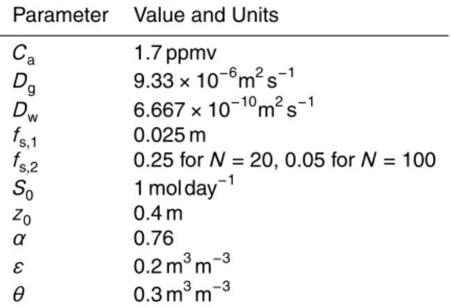
The first analytical model is the steady state CO₂diffusion model presented in Tans (1998), but we added aqueous diffusion, which was not included in his Eq. (2). The governing equation of the modified Tans model is

εDg+θDw

d

2 Cg

dz2 +Soexp

−z

z0

=0 (11)

whose solution is

5

Cg(z)=

S_o εDg+θDw

z₀2

1−exp

−z

z0

+Ca (12)

We list the parameter values used in our example application in Table 2.

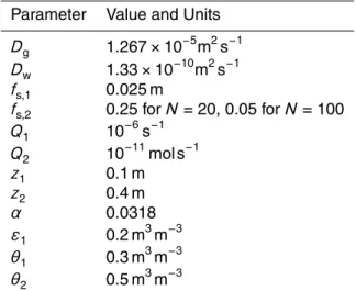
We craft the second model to mimic the methane cycle in a peatland, with methane consumption in the unsaturated topsoil (defined as from the soil surface to depthz1,

below which the soil is saturated) and a constant methane production from depthz1to

10

z2. We could have replicated published methane models and compared with pore-water

CH₄ concentrations, but other uncertainties (e.g., uncertainties in parameterization, formulation, and measurement) would obfuscate a direct evaluation of the accuracy of our diffusive transport numerical formulation.

The governing equation of the steady-state methane model is

15

ε1Dg+αθ1Dw

d

2 Cg

dz2 −Q1θ1Cw=0, for 0≤z≤z1 (13a)

(αθ2Dw)

d2Cg

∂z2 +Q2=0, forz1< z < z2 (13b)

"

ε₁D_g+αθ₁D_wdCg

dz

#

z−

1

= αθ_sD_wdCg

dz

!

z+ 1

(13c)

dCg

dz =0, forz≥z2 (13d)

(9)

BGD

11, 1587–1611, 2014

transport

Title Page Abstract Introduction Conclusions References Tables Figures ◭ ◮ ◭ ◮ Back Close

Full Screen / Esc

Printer-friendly Version Interactive Discussion Discussion P a per | D iscussion P a per | Discussion P a per | Discuss ion P a per |

whose solution is found (see Supplement) as

Cg(z)= Caexp

q_αθ

1Q1 D1 z1

−Q2

D1

q _D

1

αθ1Q1(z2−z1)

exp

−

q_αθ

1Q1 D₁ z1

+expqαθ1Q1 D₁ z1

exp 

− s

αθ1Q1 D1

z



 (14a)

+

Caexp

−

q_αθ

1Q1 D1 z1

+Q2 D1

q _D

1

αθ1Q1(z2−z1)

exp

−

q_αθ

1Q1 D₁ z1

+expqαθ1Q1 D₁ z1

exp 

 s

αθ1Q1 D1

z



, for 0≤z≤z1

Cg(z)= Q2 D2

(z−z₁) (z2−z1)− Q2

2D2

(z−z₁)2+Cg(z1) , forz1< z < z2 (14b)

5

Cg(z)= Q2

2D2

(z2−z1)2+Cg(z1) , forz≥z2 (14c)

where D₁=ε₁D_g+αθ₁D_w and D₂=αθ₂D_w. Parameter values used in our example application are listed in Table 3.

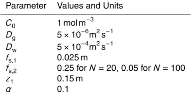
The transient model considers the release of a tracer from a constant point source

10

(C0) into a media, which is connected to another media at some distancez1. The tracer

has di_fferent di_ffusivities and solubilities in the two media, and its concentration is kept zero at the bottom of the second media. The model solves for the temporal evolution of the tracer in both media. Mathematically, the model is formulated as

∂C_g ∂t =Dg

∂2C_g

∂z2 , for 0< z < z1 (15a)

15

∂Cg

∂t =Dw

∂2Cg

(10)

BGD

11, 1587–1611, 2014

transport

Title Page

Tables Figures

◭ ◮

Back Close

Full Screen / Esc

Discussion

P

a

per

|

D

iscussion

P

a

per

|

Discussion

P

a

per

|

Discuss

ion

P

a

per

|

Dg ∂C_g

∂z

!

z−

1

= Dwα ∂C_g

∂z

!

z₁+

(15c)

Cg z+₁

=Cg z − 1

(15d)

where we note the variables in Eq. (15) are now not necessarily related to gaseous and aqueous phases, but we simply keep the denotations for simplicity. The initial condition

5

to Eq. (15) is set as zero tracer concentration everywhere inside the column.

The model represented by Eq. (15) can represent a few different problems, such as contaminant diffusion from human skin into blood (e.g., Riley et al., 2004) or heat conduction between two metals of an alloy (e.g., Carslaw and Jaeger, 1986). When all coefficients are given as constant, Eq. (15) has the analytic solution (Carslaw and

10

Jaeger, 1986):

C_g(z≤z₁)=

C0 DgL/α−Dws

DgL/α+Dwz1

−2C0 ∞

X

n=1

sin2(kLβ_n) sin (β_nz)

β_nhz1sin2(kLβn)+αLsin2(z1βn)

iexp

−D_gβ_n2t

(16a)

Cg(z≥z1)=

DgC0(L−s) DgL+Dwz1α

−2C0 ∞

X

n=1

sin (z1βn) sin (kLβn) sin (k(L−s)βn)

βn

h

z1sin2(kLβn)+αLsin2(z1βn)

i exp

−D_gβ_n2t

(16b)

15

wheres=z−z₁,k=qDg/Dw. The eigenvalues,βn, are solutions of

cos (βz1) sin (kβL)+σsin (βz1) cos (kβL)=0 (16c)

(11)

BGD

11, 1587–1611, 2014

transport

Title Page

Tables Figures

◭ ◮

Back Close

Full Screen / Esc

Discussion

P

a

per

|

D

iscussion

P

a

per

|

Discussion

P

a

per

|

Discuss

ion

P

a

per

|

which is solved by Newton iteration methods. In evaluating Eq. (16), we only used the first 17 eigenvalues, because more eigenvalues did not significantly improve the estimation. Parameter values for the example application are listed in Table 4.

In all numerical experiments, we discretized the vertical soil profile using a scheme modified from CLM4.5 (Oleson et al., 2013), which defines the node depth of layerjas

5

z_j =

(

fs,1

exp

fs,2(j−0.5)

−1 , j₌1,· · ·,N−1

2L+z_N−1

/3j=N (17a)

and the thickness of each layer as

∆zj =

  

 

0.5 (z1+z2) j=1

0.5 zj+1−zj−1

j=2, 3,· · ·,N−1

2 L−z_N₋₁/3 j=N

(17b)

and the depth at interfaces as

10

zh,j =

(

0.5 z_j+z_j₊1

j=1, 2,· · ·,N−1

zN+0.5∆zN j=N

(17c)

For all numerical experiments, the total soil column depth is set to 3.7 m. For the nu-merical approximation to the transient problem, the Crank–Nicholson method (Crank and Nicholson, 1947) is used for temporal discretization.

3 Results and discussion

15

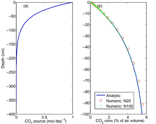
Driven by the prescribed CO2source (Fig. 2a), the numerical solution using 100

numer-ical layers predicts a soil CO2profile very close to the exact solution throughout the soil

(12)

BGD

11, 1587–1611, 2014

transport

Title Page

Tables Figures

◭ ◮

Back Close

Full Screen / Esc

Discussion

P

a

per

|

D

iscussion

P

a

per

|

Discussion

P

a

per

|

Discuss

ion

P

a

per

|

visually. Decreasing the number of numerical layers to 20 leads to visually discernible deviations from the analytic solution and the maximum relative error increases to∼4 %. However, the maximum relative error in both cases is near the surface, where the CO2

concentration is low. The 20- and 100-layer simulations predict a surface CO₂efflux of about 1 % and 0.03 % accuracy, respectively, with respect to the analytical flux. These

5

results indicate our numerical technique is sufficient for most soil dual-phase diffusion modeling applications.

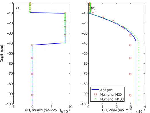
The evaluation of the CH4 numerical solution against the analytical CH4 model in

general shows good accuracy. As for CO2, more numerical layers lead to better

nu-merical accuracy. Both 20-layer and 100-layer solutions indicate significant deviations

10

from the analytical soil CH₄ profile, but the largest relative error is about 5 % for the 20-layer simulation and less than 1 % for the 100-layer simulation. The largest relative error occurs at the bottom of the topsoil (10 cm) in both cases. Because of the numeri-cal approximation, both numerinumeri-cal solutions do not have numerinumeri-cal layers interfaced at 10 cm, which, when combined with the abrupt transition from the first order

consump-15

tion in topsoil to the constant methane production rate between 10 cm and 40 cm, lead to the largest relative error. Nevertheless, considering that the 20-layer and 100-layer solutions have 7 % and 3 % relative error, respectively, in approximating the surface methane fluxes, the numerical algorithm should again satisfy the needs of modeling methane dynamics in ecosystem biogeochemical models.

20

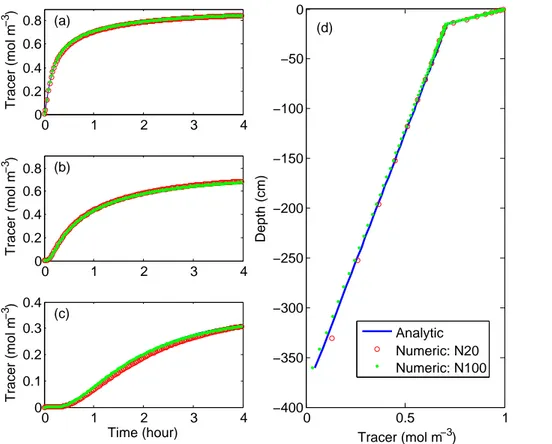
For the transient model, we first compared the temporal evolution of tracer concen-trations at three depths (7 cm, 15 cm, and 200 cm) (Fig. 4a–c, respectively). Again, both the 20-layer and 100-layer simulations show visually very accurate results (with mean relative error less than 5 % for the 20-layer and less than 1 % for the 100-layer) though there are large errors (>100 %) in the first ten minutes of the simulations (when tracer

25

concentrations are very low), which are probably caused by errors in both the finite volume approximation and the numerical error in evaluating the analytic results (see Fig. S1 for the latter case). When the steady state solutions are compared (Fig. 4d), the two numerical models show mean relative error within 2 %, indicating our numerical

(13)

BGD

11, 1587–1611, 2014

transport

Title Page

Tables Figures

◭ ◮

Back Close

Full Screen / Esc

Discussion

P

a

per

|

D

iscussion

P

a

per

|

Discussion

P

a

per

|

Discuss

ion

P

a

per

|

algorithm are very accurate. In both transient and steady state cases, the numerically predicted top surface fluxes agree with the analytical solution with a mean relative error within 10 % for the 20-layer and 2 % for the 100-layer simulations, respectively, after the first twenty minutes of simulation.

To summarize from the three evaluations, we contend Eq. (4a) and its approximation

5

Eq. (9) should be very helpful for solving the dual-phase diffusion problem.

4 Conclusion

Dual-phase diffusion is an important process that needs to be represented in depth-resolved biogeochemical models. Here we reviewed existing formulations in the litera-ture and categorized three forms used in biogeochemical models. We recommend that

10

the gas-primary form (Eq. 4a) is the most convenient to solve. Its finite volume approx-imation can represent tracer transport in variably saturated soils without the need for special treatment of the air–water interface (as is often done in existing methane mod-els). Our evaluation of the numerical algorithm with three analytical models demon-strated good accuracy of our numerical model, with some dependence on spatial

dis-15

cretization. We hope our results can help researchers develop simple but mechanistic models for some scientific questions where more complex reactive-transport models are not necessary.

Supplementary material related to this article is available online at http://www.biogeosciences-discuss.net/11/1587/2014/

20

bgd-11-1587-2014-supplement.pdf.

(14)

BGD

11, 1587–1611, 2014

transport

Title Page

Tables Figures

◭ ◮

Back Close

Full Screen / Esc

Discussion

P

a

per

|

D

iscussion

P

a

per

|

Discussion

P

a

per

|

Discuss

ion

P

a

per

|

the Next-Generation Ecosystem Experiments (NGEE Arctic) project, supported by the Office of Biological and Environmental Research in the DOE Office of Science under Contract No. DE-AC02-05CH11231.

References

Carslaw, H. S. and Jaeger, J. C.: Conduction of Heat in Solids, 2nd edn., Clarendon Press,

5

Oxford University Press, Oxford Oxfordshire, New York, viii, 510 pp., 1986.

Crank, J. and Nicolson, P.: A practical method for numerical evaluation of solutions of partial differential equations of the heat-conduction type, P. Camb. Philos. Soc., 43, 50–67, 1947. Curry, C. L.: Modeling the soil consumption of atmospheric methane at the global scale, Global

Biogeochem. Cy., 21, Gb4012, doi:10.1029/2006gb002818, 2007.

10

Davidson, E. A., Savage, K. E., Trumbore, S. E., and Borken, W.: Vertical partitioning of CO₂ production within a temperate forest soil, Glob. Change Biol., 12, 944–956, doi:10.1111/J.1365-2486.2005.01142.X, 2006.

Grant, R. F.: A review of the Canadian ecosystem model ecosys, in: Modeling Carbon and Nitrogen Dynamics for Soil Management, CRC Press, Boca, Raton, 173–264, ISBN 10:

15

1566705290, 2001.

Maggi, F., Gu, C., Riley, W. J., Hornberger, G. M., Venterea, R. T., Xu, T., Spycher, N., Steefel, C., Miller, N. L., and Oldenburg, C. M.: A mechanistic treatment of the dominant soil nitrogen cycling processes: model development, testing, and application, J. Geophys. Res.-Biogeo., 113, G02016, doi:10.1029/2007jg000578, 2008.

20

Moldrup, P., Olesen, T., Komatsu, T., Yoshikawa, S., Schjonning, P., and Rolston, D. E.: Mod-eling diffusion and reaction in soils: X. A unifying model for solute and gas diffusivity in unsaturated soil, Soil Sci., 168, 321–337, doi:10.1097/00010694-200305000-00002, 2003. Oleson, K., Lawrence, D. M., Bonan, G. B., Drewniak, B., Huang, M., Koven, C. D., Levis, S.,

Li, F., Riley, W. J., Subin, Z. M., Swenson, S., Thornton, P. E., Bozbiyik, A., Fisher, R.,

25

Heald, C. L., Kluzek, E., Lamarque, J.-F., Lawrence, P. J., Leung, L. R., Lipscomb, W., Muszala, S. P., Ricciuto, D. M., Sacks, W. J., Sun, Y., Tang, J., and Yang, Z.-L.: Techni-cal description of version 4.5 of the Community Land Model (CLM), NCAR TechniTechni-cal Note NCAR/TN-503+STR, 420 pp., doi:10.5065/D6RR1W7M, 2013.

(15)

BGD

11, 1587–1611, 2014

transport

Title Page

Tables Figures

◭ ◮

Back Close

Full Screen / Esc

Discussion

P

a

per

|

D

iscussion

P

a

per

|

Discussion

P

a

per

|

Discuss

ion

P

a

per

|

Riley, W. J., Still, C. J., Torn, M. S., and Berry, J. A.: A mechanistic model of (H2O)-O-18 and (COO)-O-18 fluxes between ecosystems and the atmosphere: model description and sensitivity analyses, Global Biogeochem. Cy., 16, 1095, doi:10.1029/2002gb001878, 2002. Riley, W. J., McKone, T. E., and Hubal, E. A. C.: Estimating contaminant dose for

intermit-tent dermal contact: model development, testing, and application, Risk Anal., 24, 73–85,

5

doi:10.1111/J.0272-4332.2004.00413.X, 2004.

Riley, W. J., Subin, Z. M., Lawrence, D. M., Swenson, S. C., Torn, M. S., Meng, L., Ma-howald, N. M., and Hess, P.: Barriers to predicting changes in global terrestrial methane fluxes: analyses using CLM4Me, a methane biogeochemistry model integrated in CESM, Biogeosciences, 8, 1925–1953, doi:10.5194/bg-8-1925-2011, 2011.

10

Simunek, J. and Suarez, D. L.: Modeling of carbon-dioxide transport and production in soil. 1. Model development, Water Resour. Res., 29, 487–497, doi:10.1029/92wr02225, 1993. Tang, J. Y. and Riley, W. J.: A new top boundary condition for modeling surface di_ffusive

ex-change of a generic volatile tracer: theoretical analysis and application to soil evaporation, Hydrol. Earth Syst. Sci., 17, 873–893, doi:10.5194/hess-17-873-2013, 2013.

15

Tang, J., Zhuang, Q., Shannon, R. D., and White, J. R.: Quantifying wetland methane emis-sions with process-based models of different complexities, Biogeosciences, 7, 3817–3837, doi:10.5194/bg-7-3817-2010, 2010.

Tang, J. Y., Riley, W. J., Koven, C. D., and Subin, Z. M.: CLM4-BeTR, a generic biogeochemical transport and reaction module for CLM4: model development, evaluation, and application,

20

Geosci. Model Dev., 6, 127–140, doi:10.5194/gmd-6-127-2013, 2013.

Tans, P. P.: Oxygen isotopic equilibrium between carbon dioxide and water in soils, Tellus B, 50, 163–178, doi:10.1034/J.1600-0889.1998.T01-1-00004.X, 1998.

Venterea, R. T. and Rolston, D. E.: Mechanistic modeling of nitrite accumulation and nitrogen oxide gas emissions during nitrification, J. Environ. Qual., 29, 1741–1751,

25

doi:10.2134/jeq2000.00472425002900060003x, 2000.

Walter, B. P. and Heimann, M.: A process-based, climate-sensitive model to derive methane emissions from natural wetlands: application to five wetland sites, sensitivity to model pa-rameters, and climate, Global Biogeochem. Cy., 14, 745–765, doi:10.1029/1999gb001204, 2000.

30

(16)

BGD

11, 1587–1611, 2014

transport

Title Page

Tables Figures

◭ ◮

Back Close

Full Screen / Esc

Discussion

P

a

per

|

D

iscussion

P

a

per

|

Discussion

P

a

per

|

Discuss

ion

P

a

per

|

with a process-based biogeochemistry model, Global Biogeochem. Cy., 18, Gb3010, doi:10.1029/2004gb002239, 2004.

Zhuang, Q. L., Chen, M., Xu, K., Tang, J. Y., Saikawa, E., Lu, Y. Y., Melillo, J. M., Prinn, R. G., and McGuire, A. D.: Response of global soil consumption of atmospheric methane to changes in atmospheric climate and nitrogen deposition, Global Biogeochem. Cy., 27, 650–

5

663, doi:10.1002/Gbc.20057, 2013.

(17)

BGD

11, 1587–1611, 2014

transport

Title Page

Tables Figures

◭ ◮

Back Close

Full Screen / Esc

Discussion

P

a

per

|

D

iscussion

P

a

per

|

Discussion

P

a

per

|

Discuss

ion

P

a

per

|

Table 1.An incomplete literature survey of different formulations that have been used for mod-eling dual-phase diffusive transport.

Equation Remark References

∂C_CH4 ∂t =∂z∂

D_i∂CCH4 ∂z

+S Bulk soil CH4concentration is the primary variable. Saturated and

unsaturated soil use different but constant diffusivitiesDi.

Walter and Heimann (2000); Zhuang et al. (2004).

∂RgCg ∂t =∂z∂

D∂Cg ∂z

+S The gaseous phase is used as primary variable. The model assumes gas diffusion to dominate in unsaturated soil and aqueous diffusion to dominate in saturated soil. The water table is assumed to be at the layer interface. Diffusivity varies continuously with soil moisture.

Venterea and Rolston (2000); Riley et al. (2011)

∂C ∂t=∂z∂ D∂C∂z

+S Bulk tracer concentration is used as the primary variable. Diff usiv-ity varies continuously with soil moisture. Special care is put to the water–air interface.

Tang et al. (2010, 2013).

∂Cg ∂t =∂z∂

Dg

∂Cg ∂z

+Sg

∂Cw ∂t=∂z∂

Dw

∂Cw ∂z

+Sw

Tracks gaseous and aqueous phase of a given tracer separately. Gas dissolution and exsolution are considered explicitly. Diffusivity varies continuously with moisture.

(18)

BGD

11, 1587–1611, 2014

transport

Title Page

Tables Figures

◭ ◮

Back Close

Full Screen / Esc

Discussion

P

a

per

|

D

iscussion

P

a

per

|

Discussion

P

a

per

|

Discuss

ion

P

a

per

|

Table 2.Parameters used for the steady-state CO₂model.

Parameter Value and Units

Ca 1.7 ppmv

D_g 9.33×10−6m2s−1

Dw 6.667×10

−10

m2s−1

fs,1 0.025 m

fs,2 0.25 forN=20, 0.05 forN=100

S₀ 1 mol day−1

z0 0.4 m

α 0.76

ε 0.2 m3m−3

θ 0.3 m3m−3

(19)

BGD

11, 1587–1611, 2014

transport

Title Page

Tables Figures

◭ ◮

Back Close

Full Screen / Esc

Discussion

P

a

per

|

D

iscussion

P

a

per

|

Discussion

P

a

per

|

Discuss

ion

P

a

per

|

Table 3.Parameters used for the steady-state CH₄model.

Parameter Value and Units

Dg 1.267×10

−5

m2s−1

Dw 1.33×10

−10

m2s−1

fs,1 0.025 m

f_s,2 0.25 forN=20, 0.05 forN=100

Q1 10

−6

s−1

Q₂ 10−11mol s−1

z₁ 0.1 m

z2 0.4 m

α 0.0318

ε₁ 0.2 m3m−3

θ₁ 0.3 m3m−3

(20)

BGD

11, 1587–1611, 2014

transport

Title Page

Tables Figures

◭ ◮

Back Close

Full Screen / Esc

Discussion

P

a

per

|

D

iscussion

P

a

per

|

Discussion

P

a

per

|

Discuss

ion

P

a

per

|

Table 4.Parameters used for the transient tracer diffusion model.

Parameter Values and Units

C₀ 1 mol m−3

Dg 5×10

−6

m2s−1

D_w 5×10−4m2s−1

f_s,1 0.025 m

f_s,2 0.25 forN=20, 0.05 forN=100

z₁ 0.15 m

α 0.1

(21)

BGD

11, 1587–1611, 2014

transport

Title Page

Tables Figures

◭ ◮

Back Close

Full Screen / Esc

Discussion

P

a

per

|

D

iscussion

P

a

per

|

Discussion

P

a

per

|

Discuss

ion

P

a

per

|

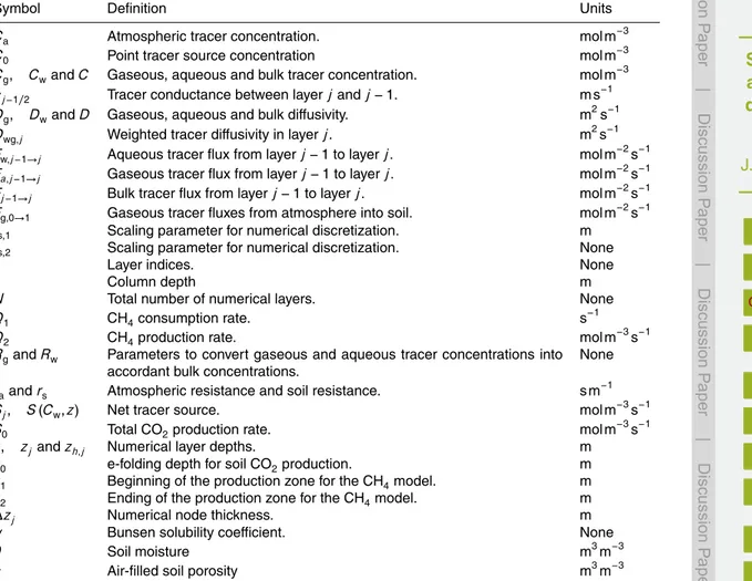
Table A1.Symbols used in paper, their definitions and corresponding units.

Symbol Definition Units

Ca Atmospheric tracer concentration. mol m

−3

C₀ Point tracer source concentration mol m−3

Cg, CwandC Gaseous, aqueous and bulk tracer concentration. mol m

−3

cj−1/2 Tracer conductance between layerjandj−1. m s

−1

Dg, DwandD Gaseous, aqueous and bulk diffusivity. m2s

−1

Dwg,j Weighted tracer diffusivity in layerj. m2s

−1

Fw,j−1→j Aqueous tracer flux from layerj−1 to layerj. mol m

−2

s−1

Fa,j−1→j Gaseous tracer flux from layerj−1 to layerj. mol m

−2

s−1

Fj−1→j Bulk tracer flux from layerj−1 to layerj. mol m

−2_s−1

F_g,0→1 Gaseous tracer fluxes from atmosphere into soil. mol m

−2

s−1

f_s,1 Scaling parameter for numerical discretization. m

fs,2 Scaling parameter for numerical discretization. None

j Layer indices. None

L Column depth m

N Total number of numerical layers. None

Q₁ CH₄consumption rate. s−1

Q2 CH4production rate. mol m

−3_s−1

R_gandR_w Parameters to convert gaseous and aqueous tracer concentrations into accordant bulk concentrations.

None

r_aandr_s Atmospheric resistance and soil resistance. s m−1

S_j, S(C_w,z) Net tracer source. mol m−3

s−1

S₀ Total CO₂production rate. mol m−3s−1

z, zjandzh,j Numerical layer depths. m

z₀ e-folding depth for soil CO₂production. m

z1 Beginning of the production zone for the CH4model. m

z₂ Ending of the production zone for the CH₄model. m

∆z_j Numerical node thickness. m

α Bunsen solubility coefficient. None

θ Soil moisture m3m−3

(22)

BGD

11, 1587–1611, 2014

transport

Title Page

Tables Figures

◭ ◮

Back Close

Full Screen / Esc

Discussion

P

a

per

|

D

iscussion

P

a

per

|

Discussion

P

a

per

|

Discuss

ion

P

a

per

|

C

_j−1

,

∆

z

_j−1

, D

_w,j−1

,D

_g,j−1

,

α

_j−1

,

θ

_j−1

,

ε

_j−1

C

j

,

∆

z

j

, D

j

,

α

j

,

θ

j

,

ε

j

,S

j

C

j+1

,

∆

z

j+1

, D

j+1

,

α

j+1

,

θ

j+1

F

w,j−1→j

F

g,j−1→j

F

_j_→_j+1

Fig. 1.Schematic of the dual-phase diffusive transport problem: solid lines are the interfaces between control volumes and the dashed line is the center of the control volume. All symbols are defined in Table A1.

(23)

BGD

11, 1587–1611, 2014

transport

Title Page

Tables Figures

◭ ◮

Back Close

Full Screen / Esc

Discussion

P

a

per

|

D

iscussion

P

a

per

|

Discussion

P

a

per

|

Discuss

ion

P

a

per

|

0 0.5 1

−400 −350 −300 −250 −200 −150 −100 −50 0

Depth (cm)

CO₂ source (mol day−1)

(a)

0 2 4 6

−100 −90 −80 −70 −60 −50 −40 −30 −20 −10 0

CO₂ conc (% of air volume)

(b)

Analytic Numeric: N20 Numeric: N100

(24)

BGD

11, 1587–1611, 2014

transport

Title Page

Tables Figures

◭ ◮

Back Close

Full Screen / Esc

Discussion

P

a

per

|

D

iscussion

P

a

per

|

Discussion

P

a

per

|

Discuss

ion

P

a

per

|

−5 0 5 10

x 10−7 −100

−90 −80 −70 −60 −50 −40 −30 −20 −10 0

Depth (cm)

CH₄ source (mol day−1) (a)

0 1 2 3 4

x 10−4 −100

−90 −80 −70 −60 −50 −40 −30 −20 −10 0

(b)

CH₄ conc (mol m−3) Analytic

Numeric: N20 Numeric: N100

Fig. 3.Comparison between the numerical and analytical solutions for the steady-state soil methane model:(a)net CH₄source profiles;(b)soil gaseous CH₄profiles. N20 indicates the solution using 20 numerical layers and N100 indicates the solution using 100 numerical layers.

(25)

BGD

11, 1587–1611, 2014

transport

Title Page

Tables Figures

◭ ◮

Back Close

Full Screen / Esc

Discussion

P

a

per

|

D

iscussion

P

a

per

|

Discussion

P

a

per

|

Discuss

ion

P

a

per

|

0 1 2 3 4

0 0.2 0.4 0.6 0.8

Tracer (mol m

−

3 ) _(a)

0 1 2 3 4

0 0.2 0.4 0.6 0.8

Tracer (mol m

−

3 ) _(b)

0 1 2 3 4

0 0.1 0.2 0.3 0.4

Time (hour)

Tracer (mol m

−

3 ) _(c)

0 0.5 1

−400 −350 −300 −250 −200 −150 −100 −50 0

Tracer (mol m−3)

Depth (cm)

(d)

Analytic Numeric: N20 Numeric: N100