Delineating riparian zones for entire river networks using geomorphological criteria

(1)

HESSD

9, 4045–4071, 2012

Delineating riparian zones for entire river

networks

D. Fern ´andez et al.

Title Page

Abstract Introduction

Conclusions References

Tables Figures

◭ ◮

Back Close

Full Screen / Esc

Printer-friendly Version Interactive Discussion

Discussion

P

a

per

|

Dis

cussion

P

a

per

|

Discussion

P

a

per

|

Discussio

n

P

a

per

|

Hydrol. Earth Syst. Sci. Discuss., 9, 4045–4071, 2012 www.hydrol-earth-syst-sci-discuss.net/9/4045/2012/ doi:10.5194/hessd-9-4045-2012

Hydrology and Earth System Sciences Discussions

This discussion paper is/has been under review for the journal Hydrology and Earth System Sciences (HESS). Please refer to the corresponding final paper in HESS if available.

Delineating riparian zones for entire river

networks using geomorphological criteria

D. Fern ández, J. Barqu´ın, M. Álvarez-Cabria, and F. J. Pe ñas

Environmental Hydraulics Institute “IH Cantabria”, Universidad de Cantabria, PCTCAN. C/ Isabel Torres 15, 39011 Santander, Spain

Received: 7 March 2012 – Accepted: 12 March 2012 – Published: 28 March 2012 Correspondence to: D. Fern ´andez (diegofgrm@gmail.com)

(2)

HESSD

9, 4045–4071, 2012

networks

Title Page

Tables Figures

◭ ◮

Back Close

Full Screen / Esc

Discussion

P

a

per

|

Dis

cussion

P

a

per

|

Discussion

P

a

per

|

Discussio

n

P

a

per

|

Abstract

Riparian zone delineation is a central issue for riparian and river ecosystem manage-ment, however, criteria used to delineate them are still under debate. The area inun-dated by a 50-yr flood has been indicated as an optimal hydrological descriptor for ripar-ian areas. This detailed hydrological information is, however, not usually available for

5

entire river corridors, and is only available for populated areas at risk of flooding. One of the requirements for catchment planning is to establish the most appropriate loca-tion of zones to conserve or restore riparian buffer strips for whole river networks. This issue could be solved by using geomorphological criteria extracted from Digital Eleva-tion Models. In this work we have explored the adjustment of surfaces developed under

10

two di_fferent geomorphological criteria with respect to the flooded area covered by the 50-yr flood, in an attempt to rapidly delineate hydrologically-meaningful riparian zones for entire river networks. The first geomorphological criterion is based on the surface that intersects valley walls at a given number of bankfull depths above the channel (BF-DAC), while the second is based on the surface defined by a threshold value indicating

15

the relative cost of moving from the stream up to the valley, accounting for slope and elevation change (path distance). As the relationship between local geomorphology and 50-yr flood has been suggested to be river-type dependant, we have performed our analyses distinguishing between three river types corresponding with three valley morphologies: open, shallow vee and deep vee valleys (in increasing degree of valley

20

constrainment). Adjustment between the surfaces derived from geomorphological and hydrological criteria has been evaluated using two different methods: one based on ex-ceeding areas (minimum exex-ceeding score) and the other on the similarity among total area values. Both methods have pointed out the same surfaces when looking for those that best match with the 50-yr flood. Results have shown that the BFDAC approach

25

(3)

HESSD

9, 4045–4071, 2012

networks

Title Page

Tables Figures

◭ ◮

Back Close

Full Screen / Esc

Discussion

P

a

per

|

Dis

cussion

P

a

per

|

Discussion

P

a

per

|

Discussio

n

P

a

per

|

constrained valleys when deriving surfaces using geomorphological criteria. Moreover, this study provides: (i) guidance on the selection of the proper geomorphological crite-rion and associated threshold values, and (ii) an easy calibration framework to evaluate the adjustment with respect to hydrologically-meaningful surfaces.

1 Introduction

5

Riparian vegetation is involved in different geomorphological, hydrological and ecologi-cal processes (Tabacchi et al., 1998; Naiman et al., 2005) and provides many services to society, such as reducing flood risk or improving the availability and quality of water (Staats and Holtzman, 2002; Hruby, 2009). Despite this, riparian zones are commonly under high pressure due to human activities and land-use transformation (for a review

10

see Po_ffet al., 2011). The maintenance of riparian functions and values is of key im-portance and requires planning at catchment scale and to locate the optimal zones to conserve or restore riparian buffer strips. Additionally, the definition of riparian zone ex-tent is an unavoidable issue when managing river corridors. There are however, several different approaches to delineate riparian areas and consensus is still far from being

15

achieved.

The delineation of riparian zones is highly dependant on what is understood as “ri-parian”. Existing definitions are quite heterogeneous with respect to the zones encom-passed by this term. While most authors use definitions matching with river banks and floodplains, others also include river channels (Naiman et al., 1993; USDA FS,

20

1994) or extend these zones to the slopes adjacent to floodplains (Ilhardt et al., 2000; Verry et al., 2004). By focusing on land adjacent to watercourses, there is agreement about the following riparian zone characteristics: (i) they are transitional zones between aquatic and terrestrial ecosystems (Gregory et al., 1991; NRC, 2002), (ii) their soil and vegetation characteristics are strongly influenced by free or unbound water in the soil

25

(4)

envi-HESSD

9, 4045–4071, 2012

networks

Title Page

Tables Figures

◭ ◮

Back Close

Full Screen / Esc

Discussion

P

a

per

|

Dis

cussion

P

a

per

|

Discussion

P

a

per

|

Discussio

n

P

a

per

|

ronmental factors, ecological processes and biota (Gregory et al., 1991; NRC, 2002). As an ecotone, riparian zone limits are fuzzy and defining discrete boundaries can be a difficult task. In addition, the extent of the riparian zone is not constant within the longitudinal dimension of rivers, nor follows a well-established increasing gradient from source to mouth. Instead, riparian vegetation responds to the array of

hydrogeomor-5

phic patches appearing along the fluvial network (Van Coller et al., 2000; Poole, 2002; Thorp et al., 2006), being influenced by the external disturbance regimes of floods and landslides (Gregory et al., 1991) and also by channel confluences (Benda et al., 2004).

As Yarrow and Mar´ın (2007) suggest, a compromise is made when we move from

theoretical to operational definitions. Establishing fixed distances from water edge has

10

been a common approach in riparian delineation for regulatory purposes (e.g. best management practices, Australian Rivers and Foreshores Improvement Act, Canadian Streamside Protection Regulation), with buffer widths ranging habitually from 10 to less than 50 m. In this regard, 40 m is suggested by some authors as the width that ac-complishes most riparian functions (Sutula et al., 2006, Clerici et al., 2011). However,

15

other authors point out the maintenance of wildlife at that width is only assured for aquatic species, but do not encompass the zone of primary activity of amphibians and terrestrial species (Pearson and Manuwal, 2001; Hruby 2009). Moreover, headwater

streams have been suggested to require much narrower buffer strips to ensure

am-phibians support (Perkins and Hunter, 2006). In this line, fixed bu_ffer approaches often

20

result in oversized riparian areas in headwaters and confined valleys and undersized in lowlands and unconfined valleys (Holmes and Goebel, 2011). Some authors have dealt with this issue by establishing a bu_ffer distance dependant on river order (e.g., Yang et al., 2007), although this approach is still not sensitive to local geomorphology as a river of a given order can show large valley morphology variability. Recent

ap-25

(5)

HESSD

9, 4045–4071, 2012

networks

Title Page

Tables Figures

◭ ◮

Back Close

Full Screen / Esc

Discussion

P

a

per

|

Dis

cussion

P

a

per

|

Discussion

P

a

per

|

Discussio

n

P

a

per

|

2003; Mac Nally et al., 2008) or amphibians (Perkins and Hunter, 2006). Most of these criteria demand information that is not usually available over large areas, or not with enough spatial resolution to delineate riparian areas. Besides, they are usually applied to definite linear boundaries without accounting for the environmental gradients existing within riparian zones. Instead, Clerici et al. (2011) have developed a GIS-based riparian

5

zonation model which uses membership scores indicating the probability of belonging to the riparian zone based on natural vegetation presence and water influence.

Riparian vegetation communities have di_fferent composition and phenologies than

those present in upland zones, and their spatial and temporal distribution is heavily influenced by flood regime (Merrit et al., 2009; Naura et al., 2011). High flows

(char-10

acterised by magnitude, duration and frequency) control the creation and destruction of landforms across the fluvial landscape, and limit the spread of non-riparian species (Merrit et al., 2009). Consequently, flood recurrence interval may be an objective ap-proach to delineate the outward boundary of the riparian zone. In this regard, the 50-yr flood has been indicated as an appropriate hydrological descriptor for riparian zones as

15

it usually coincides with the first terrace or other upward sloping surface (Ilhardt et al., 2000). Moving outward this topographic boundary necessarily increases water table depth and the probability of finding vegetation species related to riparian ecosystems may rapidly decrease. Deriving the surface covered by a flood of a given recurrence interval, however, requires long series of flow data (failing that, it requires long series

20

of precipitation data and information about catchment response to precipitation) and valley and channel cross-section data at many locations. This issue can be solved us-ing geomorphological criteria potentially related to hydrology. Geographical Information Systems (GIS) allow the application of these geomorphological criteria over large ar-eas from few ar-easily-available inputs (e.g., Digital Elevation Model; DEM). Unfortunately,

25

there are not many published works dealing with this issue and the existing ones follow

different methodological approaches (e.g., Sutula et al., 2006; Abood and Maclean,

(6)

HESSD

9, 4045–4071, 2012

networks

Title Page

Tables Figures

◭ ◮

Back Close

Full Screen / Esc

Discussion

P

a

per

|

Dis

cussion

P

a

per

|

Discussion

P

a

per

|

Discussio

n

P

a

per

|

the adjustment of two geomorphological criteria, the number of bankfull depths above the channel (BFDAC) and the path distance, with respect to the 50-yr flood in a GIS environment. This is intended to rapidly delineate hydrologically-meaningful riparian zones for entire river networks. As the relationship between local geomorphology and 50-yr flood has been suggested to be river-type dependant (Rosgen, 1996) we have

5

performed the analyses distinguishing between three river types corresponding with three valley morphologies: (i) open valleys, (ii) shallow-vee valleys and (iii) deep-vee

valleys and gorges. We have also compared the performance of two di_fferent

meth-ods to evaluate adjustment between the surfaces derived from geomorphological and hydrological criteria. One of them is based on exceeding areas (minimum exceeding

10

score) and the other on the similarity among total area values.

2 Material and methods

2.1 Study area

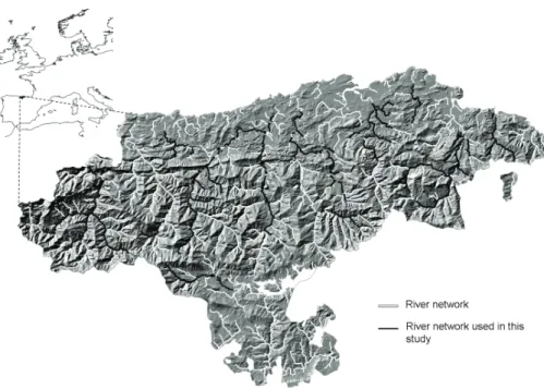
This study was developed in river catchments from the Cantabrian region, Northern Spain. Only river stretches with no flood restrictions for which flood data (specifically,

15

surface flooded by the 50-yr flood) was available have been included in the study (Fig. 1). Cantabrian rivers have their source in the Cantabrian Cordillera, a mountain range which runs parallel to the Atlantic Ocean coast and reaches up to 2600 m a.s.l. In the northern part of the region, rivers drain into the Atlantic Ocean. These rivers are short, with high slopes and high erosive power. The largest basins slightly exceed

20

1000 km2and 20 m3s−1_{of mean daily flow, with highly variable valley widths that rarely} exceed 1.5 km in most of the middle and upper courses. This area has a humid oceanic temperate climate (Rivas-Mart´ınez et al., 2004) with an average annual temperature of 14◦_{C and an average annual precipitation of 1200 mm. The southern part of Cantabria} is dominated by a continental climate with an average annual temperature of 10◦_{C and}

25

(7)

ex-HESSD

9, 4045–4071, 2012

networks

Title Page

Tables Figures

◭ ◮

Back Close

Full Screen / Esc

Discussion

P

a

per

|

Dis

cussion

P

a

per

|

Discussion

P

a

per

|

Discussio

n

P

a

per

|

tensive and complex river systems which flow into the Mediterranean and the Atlantic, and they present more gentle relief and wider maximum valley widths than northern basins. In this area, rivers are generally long and with a gentle slope, draining into the Atlantic Ocean (Duero river basin) and into the Mediterranean Sea (Ebro river basin). The riparian vegetation is dominated by oceanic alder groves (Alnus glutinosa) in the

5

Atlantic draining catchments from almost sea level up to 700 m and by submediter-ranean alder groves (Alnus glutinosa) in the southern draining catchments (Lara et al.,

2004). Willow groves formed bySalix atrocinerea(Northern Cantabrian cordillera) and

S. cantabrica(Southern Cantabrian cordillera) replace alder groves when they deteri-orate, soils are not deep enough or there are large flow fluctuations. Higher in altitude,

10

ashes (F. excelsior) or hazelnuts (C. avellana) might dominate riparian forest, while in steep valleys beech, oak and mixed Atlantic forest predominate. Finally, when riparian forests are impaired by human activities, the riparian vegetation is usually dominated byRubus sp.,Rosa sp.,Crataegus monogyna, Prunus spinosaor even pasture forma-tions. For a more detailed description of the study area see (Barqu´ın et al., 2012)

15

2.2 Defining river network and river types

The geomorphological criteria used in this study requires a river network with the fol-lowing geomorphological attributes: bankfull depth, channel and riverbank slope, valley floor width and riverbank geological hardness (considering as riverbank zone a buffer of 200 m from the river channel), as all these attributes are related with the flood height

20

at a given location. This information is necessary to (i) classify the river network in morphological types and (ii) delimitate the riparian zone under the BFDAC approach. Thus, channel slope is important to distinguish among high-energy straight rivers and low-energy meandering rivers. Both riverbank slope and valley floor width characterise cross-section topography for each river reach. As valley floor width is difficult to define

25

(8)

eren-HESSD

9, 4045–4071, 2012

networks

Title Page

Tables Figures

◭ ◮

Back Close

Full Screen / Esc

Discussion

P

a

per

|

Dis

cussion

P

a

per

|

Discussion

P

a

per

|

Discussio

n

P

a

per

|

tiates those locations where river flows across alluvial easily-erodible material from those flowing across hard di_fficult-erodible geological substrate.

The river network and its geomorphological attributes were derived using the anal-ysis toolkit “NetMap” (http://www.netmaptools.org; Benda et al., 2007, 2009) following the procedure described by Benda et al. (2011). Hence, the network was delineated

us-5

ing flow directions inferred from a 5-m DEM, using the algorithms described by Clarke et al. (2008). In flat areas, DEMs usually contain cells that are completely surrounded by other cells at the same or higher elevation. These cells act as sinks to overland flow when deriving a river network using flow direction (Martz and Garbrecht, 1998). To solve this problem, we enforced drainage in low relief areas using GIS data on channel

10

locations. Then the channel network was divided into a set of channel segments (500– 1000 m) and split at confluences, as they are supposed to produce changes in channel and floodplain morphologies (Benda et al., 2004). This resulted in a set of stretches ranging from 3 to 850 m. Next, channel slope and riverbank slope were calculated at the endpoint of each segment from the DEM. Bankfull depth (BFD) was estimated

us-15

ing a regional regression of drainage area (A_{) and mean annual precipitation (}P_{) to field} measured depths over a range of channel sizes encompassing 195 river sites in the region of Cantabria (selected in areas with little to no engineered works). The results of this analysis yielded the following equation (Eq. 1):

BFD = 0.63A0.1731P0.1516 ₍₁₎

20

Valley floor width was obtained from a DEM-derived raster. Each cell in this raster was associated with the closest river segment (in Euclidean distance) presenting the fewest and smallest intervening high points. Cell values showed the elevation diff er-ence (in terms of bankfull depth) among the cell and its associated channel. Using this raster, valley width at an elevation equivalent of two bankfull depths was assessed

25

(9)

HESSD

9, 4045–4071, 2012

networks

Title Page

Tables Figures

◭ ◮

Back Close

Full Screen / Esc

Discussion

P

a

per

|

Dis

cussion

P

a

per

|

Discussion

P

a

per

|

Discussio

n

P

a

per

|

we assigned them a numerical value based on geological hardness (see Snelder et al., 2008). Finally, we obtained riverbank hardness for each river reach using NetMap tools. Channel and riverbank slope, valley floor width and riverbank geological hardness were used to classify the river network in three geomorphological types by using PAM (partition around medoids) clustering in R software (R Development Core Team, 2008),

5

previous data standardization.

2.3 Hydrological criterion and river network pruning

The area flooded by the 50-yr flood was available from a previous flood risk assess-ment study in the study area (IH Cantabria, 2008). In this study hydrological modelling with HEC MHS (US Army Corps of Engineers, 2000) was used to derive flow data.

10

This model required a high resolution DEM, a long series of precipitation data and

in-formation about land-use and soil type to quantify runoffand catchment response to

precipitation. For each river basin, flow was calculated at several points that were rep-resentative of homogeneous sub-basins. On the other hand, river hydraulics modelling was performed using HEC-RAS (US Army Corps of Engineers, 2005) and HEC-Geo

15

RAS module, which allows use of a DEM to derive required cross-section data. This model requires as input several parameters influencing flow behaviour: Manning’s num-ber, coe_fficients of expansion and contraction and boundary conditions.

As there is no human development in the upper reaches, the 50-yr flood was not available for headwaters (Strahler order 1 and 2). From the 427 km where this

infor-20

(10)

HESSD

9, 4045–4071, 2012

networks

Title Page

Tables Figures

◭ ◮

Back Close

Full Screen / Esc

Discussion

P

a

per

|

Dis

cussion

P

a

per

|

Discussion

P

a

per

|

Discussio

n

P

a

per

|

2.4 Surfaces derived from geomorphological criteria

GIS provides a fast technique to produce surfaces which are sensitive to stream bank topography. The main inputs to carry out this task are a DEM and a stream line. We used the DEM and streamline cited in Sect. 2.2 to apply two geomorphological ap-proaches: the BFDAC and the path distance.

5

The bankfull discharge is the flow that fills a stream channel to the elevation of the active floodplain (Wolman and Leopold, 1957). The vertical distance from the deepest part of a channel to the bankfull elevation is called the bankfull depth. The area border-ing a stream that will be covered by water at a flood stage of twice the maximum bank-full depth is called the floodprone area and corresponds on average to that which gets

10

flooded by the 50-yr flood (Rosgen, 1996). However, floodprone height ranges from 1.3 times the bankfull depth in rivers of Rosgen’s type E (low-gradient meandering rivers) to 2.7 times the bankfull depth in rivers of type A (highly-entrenched streams), and generally includes the active floodplain and the low terrace (Rosgen, 1996). Based on Rosgen’s empirical data, valley width as considered in this study (valley width at

15

a height of 2 times the bankfull depth) must coincide with the surface flooded by 50-yr flood. However, this relationship may be different when modelling in a GIS environ-ment. To analyse this, we developed several surfaces calculated from different BFDAC heights and then we compared their adjustment with the 50-yr flood. These surfaces were obtained following the same procedure described for the valley floor surface in

20

Sect. 2.2 and using different bankfull depth heights ranging from 0.25 to 3 using steps of 0.25.

The path distance is a surface of values indicating the relative costs of moving from the stream cells up into the stream valley, accounting for slope and elevation change. It only requires a stream line and a DEM to be assessed. Path distance surface (raster

25

(11)

HESSD

9, 4045–4071, 2012

networks

Title Page

Tables Figures

◭ ◮

Back Close

Full Screen / Esc

Discussion

P

a

per

|

Dis

cussion

P

a

per

|

Discussion

P

a

per

|

Discussio

n

P

a

per

|

This has been done by reclassifying path distance raster using the above-mentioned threshold values and converting raster into polygon (shapefile).

Therefore, several surfaces (in ArcGIS polygon shapefile format) were derived for each geomorphological approach (Fig. 3). Hereafter we will refer to them as geo-morphological surfaces. Those derived following the BFDAC are cited in the text as

5

BFD×X, beingX the factor multiplying bankfull depth (e.g. BFD×1.25). On the other

hand, geomorphological surfaces derived using the path distance approach are cited as PD-Y, beingY the threshold value used to generate that surface (e.g. PD-250).

2.5 Data analyses

Each geomorphological surface was fragmented based on river type using ArcGis

soft-10

ware (ESRI, 2011) and the total area in each type was calculated. To evaluate the adjustment of each surface with respect to the 50-yr flood we have used two di_fferent methods:

(i) Minimum exceeding score (Eq. 2). This method combines the two possible ex-ceeding surfaces: geomorphological surface exex-ceeding area (GSEA) and 50-yr

15

flood exceeding area (T50EA; Fig. 4). GSEA is the area of the geomorphologi-cal surface exceeding the 50-yr flood, while the T50EA is the area of the 50-yr flood not covered by the geomorphological surface. This latter parameter results from subtracting the coinciding area (CA; Fig.4) from the 50-yr flood. The optimal geomorphological surface is that achieving the lowest minimum exceeding score.

20

Minimum exceeding score = T50EA +GSEA

100 (2)

(ii) Total area (Eq. 3). This method does not look at coinciding or exceeding areas, but only considers the deviance between the value of the area occupied by the geomorphological surface and the value of the area covered by the 50-yr flood.

(12)

HESSD

9, 4045–4071, 2012

networks

Title Page

Tables Figures

◭ ◮

Back Close

Full Screen / Esc

Discussion

P

a

per

|

Dis

cussion

P

a

per

|

Discussion

P

a

per

|

Discussio

n

P

a

per

|

Total area optimum value is 100, and values above or below are considered as deviations. This condition may not reflect an “optimum adjustment”, but as all geomorphological surfaces and the 50-yr flood are supposed to be sensitive to geomorphology, we have considered exploring this possibility.

Total area = geomorphological surface total area

area covered by the 50-yr flood × 100 (3)

5

3 Results

Cluster analysis resulted in three well defined groups (Fig. 2). The first of them in-cluded 1782 cases and corresponded with open valleys, as it presented the widest valleys (average>200 m), the lowest geological hardness and the lowest channel and stream bank (average of 6 degrees and 13 %, respectively) slopes. The second one

10

encompassed 1953 cases and corresponded with shallow-vee valleys presenting inter-mediate characteristics between groups 1 and 3. Finally, the third group included 1908 cases and corresponded with deep-vee valleys and gorges, as it showed narrower

val-ley widths (average<_{50 m), high geological hardness and the steepest channel and}

stream bank slopes (average of 22 degrees and 50 %, , respectively).

15

All geomorphological surfaces were sensitive to valley morphology, being narrower in constrained valleys due to closer and steeper slopes (Fig. 3). By incrementing the factor multiplying bankfull depth or the path distance threshold value, geomorpholog-ical surfaces became wider and filled those gaps that lower threshold values can not fill (corresponding with low hills located in the valley bottom). The path distance

ap-20

proach produced wider surfaces than BFDAC in unconstrained valleys, while the oppo-site trend was found in constrained valleys.

The adjustment between geomorphological and hydrological criteria, in terms of co-inciding and exceeding areas (Fig. 4), showed the same general trend for all river types and the two geomorphological criteria (Fig. 5). As it was expected, increasing

(13)

HESSD

9, 4045–4071, 2012

networks

Title Page

Tables Figures

◭ ◮

Back Close

Full Screen / Esc

Discussion

P

a

per

|

Dis

cussion

P

a

per

|

Discussion

P

a

per

|

Discussio

n

P

a

per

|

the geomorphological surface (by increasing the factor multiplying bankfull depth or increasing the path distance threshold value) increased CA, and therefore decreased T50EA. However, increasing the geomorphological surface also increased GSEA. Be-sides, the rate of increase of GSEA was greater than that of CA, except in deep-vee valleys, where they presented almost the same rate. Intersection between the T50EA

5

and the GSEA graphically indicates the minimum exceeding score optimal geomorpho-logical surface. This intersection occurred at larger geomorphogeomorpho-logical surfaces when moving from open valleys to more entrenched ones, although there are no di_fferences between open and shallow vee valleys when using the BFDAC approach. Despite the homogeneity in the above cited trends, the BFDAC reaches higher CA values than

10

path distance. Consequently, path distance reaches higher T50EA values than BFDAC. However, both approaches show similar values for GSEA.

Both minimum exceeding score and total area indicated the same or close optimal geomorphological surfaces (Fig. 6) for each valley type. When using minimum exceed-ing score, all the considered geomorphological surfaces produced values closer to

15

the optimum in deep vee valleys (which is reflected by 4 different geomorphological surfaces for BFDAC and by 2 surfaces for path distance). However, in open valleys increasing geomorphological surface causes rapid deviation from the optimum value, while shallow vee valleys presented intermediate pattern between open and deep vee valleys. The total area method showed a positive linear relationship between the value

20

defining the geomorphological surface and its total area. The slope of this relationship became steeper when moving from deep vee to open valleys. The BFDAC that best

matched the 50-yr flood was BFD×0.5 in open and shallow vee valleys, while in deep

vee valleys it was around BFD×1.25. When using path distance, optimal

geomorpho-logical surfaces were close to PD-100 in open and shallow vee valleys and around

25

(14)

HESSD

9, 4045–4071, 2012

networks

Title Page

Tables Figures

◭ ◮

Back Close

Full Screen / Esc

Discussion

P

a

per

|

Dis

cussion

P

a

per

|

Discussion

P

a

per

|

Discussio

n

P

a

per

|

4 Discussion and conclusion

Our aim of easily obtaining a 50-yr-flood-matching riparian zone by using geomorpho-logical criteria was fully achieved by merging the optimal geomorphogeomorpho-logical surface for each valley type. Calibration was needed to provide the boundaries of geomorphologi-cal surfaces with hydrologigeomorphologi-cal meaning, because GIS-derived thresholds can differ from

5

those established by empirical studies. Our calibration framework took into account the influence of the following parameters: geomorphological criterion, valley type and ad-justment assessment method. All of these parameters are discussed below. However, attention should be paid when using DEMs with a spatial resolution different from that used in this study, as thresholds are suggested to be also dependant on this parameter

10

(Sutula et al., 2006; Abood and Maclean, 2011).

Regarding geomorphological criteria performance, BFDAC and path distance seem two be valid approaches to delineate riparian areas, both presenting the advantage of being sensitive to floodplain morphology. Optimal geomorphological surfaces for BFDAC correspond with slightly higher CA (5–16 % depending on valley type) and

15

slightly lower GSEA (0–20 %) and T50EA (5–16 %) than those for path distance. This is an advantage of BFDAC approach. However, path distance does not require bankfull depth values for each river reach in the network and it can be rapidly calculated in GIS. Therefore, the choice of the proper geomorphological criterion depends on the resources and accuracy required in the study. Besides, both BFDAC and path distance

20

present the advantage that can be used to account for the gradients present in riparian

zones by assigning membership scores to each band defined by a different threshold

value (the lesser is the threshold value, the higher must be the membership score as the river influence is also higher).

Despite of differing in characteristics as streamside slope or valley width, there is no

25

(15)

HESSD

9, 4045–4071, 2012

networks

Title Page

Tables Figures

◭ ◮

Back Close

Full Screen / Esc

Discussion

P

a

per

|

Dis

cussion

P

a

per

|

Discussion

P

a

per

|

Discussio

n

P

a

per

|

it is necessary to use a different geomorphological surface for deep vee valleys and gorges because they require wider surfaces than unconstrained valleys to match with the 50-yr flood, as described by Rosgen (1996). Moreover, the worst adjustment be-tween hydrological and morphological surfaces, showed by maximum combinations of the two exceeding surfaces (T50EA and GSEA), occurred in open valleys. The same

5

result was obtained by Sutula et al. (2006). This may be due to the fact that uncon-strained valleys present more complex fluvial landscapes than conuncon-strained ones. We have also considered that tributary confluences may also partly explain the disarrange-ment between geomorphological surfaces and the 50-yr flood, as in general terms they result in lower channel gradients and wider channel and floodplains (Benda et al., 2004;

10

Fig. 7a) and they have not been considered in defining river types. However, within the study area we found many examples of confluences of the main channel with large tributaries where confluence effects are much less determinant of floodplain width than topographic constrains such as steep riverbank slopes or hardly-erodible riverbank materials (e.g., Fig. 7b, where the main channel is the Deva River and Quiviesa and

15

Bull ´on are large tributaries). Hence, it does not seem appropriate to include a variable accounting for confluence effects when classifying valley type, at least in mountainous study areas such as the one included in here. In addition, we do find larger fluvial land-scapes immediately above and below valley constrictions (Fig. 7c), as commented in Benda et al. (2001).

20

The two methods used to select the optimal geomorphological surfaces provided al-most the same result, despite the fact that total area is more subjective than minimum exceeding score. Both approaches can therefore be used to determine the geomor-phological surface that best matches the 50-yr flood, or to evaluate the adjustment between any other two surfaces. Attention should however, be paid when using the

25

(16)

HESSD

9, 4045–4071, 2012

networks

Title Page

Tables Figures

◭ ◮

Back Close

Full Screen / Esc

Discussion

P

a

per

|

Dis

cussion

P

a

per

|

Discussion

P

a

per

|

Discussio

n

P

a

per

|

causes rapid deviation from 100 % of total area, and this is reflected in exceeding and coinciding area combinations away from the optimum.

In conclusion, our results suggest that using GIS to delineate sensitive-to-geomorphology hydrologically-meaningful riparian zones is feasible and relatively easy and fast. This task does however, require local calibration in order to find an optimal

5

threshold value for the geomorphological criterion which maximizes the coinciding and minimizes the exceeding with respect to the hydrological surface. Our results also con-firmed that this optimal value is valley-type dependent, as deep vee valleys and gorges require higher threshold values than shallow vee and open valleys.

Acknowledgements. We would like to thank to Lee Benda and Daniel Miller (Earth Systems

10

Institute, CA, USA) for their collaboration and support at different stages of this research. We also thank Ben P. Gouldby for the linguistic revision of the manuscript. This study was partly funded by the Spanish Ministry of Science and Innovation as part of the project MARCE (Ref: CTM-2009-07447) and by the Program of Postdoctoral Fellowships for Research Activities of the University of Cantabria (published by resolution on 17 January 2011).

15

References

Abood, S. and Maclean, A.: Modeling riparian zones utilzing DEMs, flood height data, digital soil data and wetland inventory via GIS, in: American Society of Photogrammetry and Remote Sensing (ASPRS) 2011 Annual Conference, edited by: ASPRS, Milwaukee, Wisconsin, USA, 1–5 May 2011, 2011.

20

Amundsen, K. J.: Mapping Riparian Vegetation in the Lower Colorado River Using Low Reso-lution Satellite Imagery, Cleveland State University, USA, 2003.

Barqu´ın, J., Ondiviela, B., Recio, M., Álvarez-Cabria, M., Pe ñas, F. J., Fern ández, D., G ómez, A., Álvarez C., and Juanes, J. A.: Assessing the conservation status of alder-ash alluvial forest and Atlantic salmon in the Natura 2000 river network of Cantabria, Northern

25

(17)

HESSD

9, 4045–4071, 2012

networks

Title Page

Tables Figures

◭ ◮

Back Close

Full Screen / Esc

Discussion

P

a

per

|

Dis

cussion

P

a

per

|

Discussion

P

a

per

|

Discussio

n

P

a

per

|

Benda, L., Poff, N. L., Miller, D., Dunne, T., Reeves, G., Pess, G., and Pollock, M.: The network dynamics hypothesis: how channel networks structure riverine habitats, Bioscience, 54, 413– 427, 2004.

Benda, L., Miller, D., Andras, K., Bigelow, P., Reeves, G., and Michael, D.: NetMap: a new tool in support of watershed science and resource management, Forest Sci., 53, 206–219, 2007.

5

Benda, L., Miller, D., Lanigan, S., and Reeves, G.: Future of applied watershed science at regional scales, Eos Transactions AGU, 90, p. 156, doi:10.1029/2009EO180005, 2009. Benda, L., Miller, D., and Barqu´ın, J.: Creating a catchment scale perspective for river

restora-tion, Hydrol. Earth Syst. Sci., 15, 2995-3015, doi:10.5194/hess-15-2995-2011, 2011. Clarke, S. E., Burnett, K. M., and Miller, D. J.: Modeling streams and hydrogeomorphic attributes

10

in Oregon from digital and field data, J. Am. Water Resour. As., 44, 459–477, 2008.

Clerici, N., Weissteiner, C. J., Paracchini, M. L., and Strobl, P.: Riparian zones: where green and blue networks meet. Pan-European zonation modelling based on remote sensing and GIS, Joint Research Centre of the European Comission, Luxembourg, Technical Report, 60 pp., 2011.

15

Environmental Systems Research Institute (ESRI): ArcGIS Desktop: Release 10, Environmen-tal Systems Research Institute, Redlands, CA, USA, 2011.

Gregory, S. V., Swanson, F. J., McKee, W. A., and Cummins, K. W.: An ecosystem perspective of riparian zones, Bioscience, 41, 540–551, 1991.

Hawes, E. and Smith, M.: Riparian Buffer Zones: Functions and Recommended Widths,

Eight-20

mile River Wild and Scenic Study Committee, 15, Yale School of Forestry and Environmental Studies, April 2005.

Holmes, K. L. and Goebel, P. C.: A functional approach to riparian area delineation using geospatial methods, J. Forest., 109, 233–241, 2011.

Hruby, T.: Developing rapid methods for analyzing upland riparian functions and values,

Envi-25

ron. Manage., 43, 1219–1243, 2009.

IH Cantabria: Desarrollo de la documentaci ón t écnica y cartogr áfica para la redacci ón del plan de protecci ón civil ante el riesgo de inundaciones de la Comunidad Aut ónoma de Cantabria, Direcci ón General de Protecci ón Civil, Consejer´_ıa de Presidencia, Gobierno de Cantabria, Santander, Spain, Technical Report, 12 pp., 2008.

30

(18)

HESSD

9, 4045–4071, 2012

networks

Title Page

Tables Figures

◭ ◮

Back Close

Full Screen / Esc

Discussion

P

a

per

|

Dis

cussion

P

a

per

|

Discussion

P

a

per

|

Discussio

n

P

a

per

|

Ilhardt, B. L., Verry, E. S., and Palik, P. J.: Defining riparian areas, in: Riparian Management in Forests of the Continental Eastern United States, edited by: Verry, E. S., Hornbeck, J. W., and Dollof, C. A., Lewis Publishers, Boca Raton, Florida, USA, 2000.

Lara, F., Garilleti, R., and Calleja, J. A.: La vegetaci ´on de ribera de la mitad norte Espa ˜nola, Monografias, 81, 536, 2004.

5

Mac Nally, R., Molyneux, G., Thomson, J. R., Lake, P. S., and Read, J.: Variation in widths of riparian-zone vegetation of higher-elevation streams and implications for conservation man-agement, Plant Ecol., 198, 89–100, 2008.

Martz, L. W. and Garbrecht, J.: The treatment of flat areas and depressions in automated drainage analysis of raster digital elevation models, Hydrol. Process., 12, 843–855, 1998.

10

Merritt, D. M., Scott, M. L., Poff, N. L., Auble, G. T., and Lytle, D. A.: Theory, methods and tools for determining environmental flows for riparian vegetation: riparian vegetation-flow response guilds, Freshwater Biol., 55, 206–225, 2009.

Naiman, R. J., Decamps, H., and Pollock, M.: The role of riparian corridors in maintaining regional biodiversity, Ecol. Appl., 3, 209–212, 1993.

15

Naiman, R. J., D ´ecamps, H., and McClain, M.: Riparia: Ecology, Conservation, and Manage-ment of Streamside Communities, Elsevier Academic Press, 430, San Diego, California, USA, 2005.

National Research Council (NRC), Committee on Riparian Zone Functioning and Strategies for Management: Riparian areas: functions and strategies for management, National Academy

20

Press, Washington, DC, USA, 444, 2002.

Naura, M., Sear, D., Álvarez-Cabria, M., Pe ñas, F. J., Fern ández, D., and Barqu´ın, J.: Integrating monitoring, expert knowledge and habitat management within conservation organisations for the delivery of the water framework directive: a proposed approach, Limnetica, 30, 427–446, 2011.

25

Osterkamp, W. R. and Hupp, C. R.: Fluvial processes and vegetation – glimpses of the past, the present, and perhaps the future, Geomorphology, 116, 274–285, 2010.

Palik, B. J., Tang, S. M., and Chavez, Q.: Estimating riparian area extent and land use in the Midwest, Gen. Tech. Rep. NC-248., Department of Agriculture, Forest Service, North Central Research Station, St. Paul, MN, 28, 2004.

30

(19)

HESSD

9, 4045–4071, 2012

networks

Title Page

Tables Figures

◭ ◮

Back Close

Full Screen / Esc

Discussion

P

a

per

|

Dis

cussion

P

a

per

|

Discussion

P

a

per

|

Discussio

n

P

a

per

|

Perkins, D. W. and Hunter, M. L.: Use of amphibians to define riparian zones along headwater streams in Maine, Can. J. Forest. Res., 36, 2124–2130, 2006.

Poff, B., Koestner, K. A., Neary, D. G., and Henderson, V.: Threats to riparian ecosystems in Western North America: an analysis of existing literature, J. Am. Water Resour. As., 47, 1241–1254, 2011.

5

Poole, G. C.: Fluvial landscape ecology: addressing uniqueness within the river discontinuum, Freshwater Biol., 47, 641–660, 2002.

R Development Core Team: R: A language and environment for statistical computing, Vienna, Austria, software 3-900051-07-0, 2008.

Rivas-Mart´ınez, S., Penas, A., and D´ıaz, T. E.: Bioclimatic Map of Europe, in: Bioclimates, Le ´on

10

University, Cartographic Service, Le ´on, Spain, 2004.

Rosgen, D. L.: Applied river morphology, Wildland Hydrology, Pagosa Springs, CO, USA, 1996. Snelder, T., Pella, H., Wasson, J.-G., and Lamouroux, N.: Definition procedures have little effect

on performance of environmental classifications of streams and rivers, Environ. Manage., 42, 771–788, 2008.

15

Staats, J. and Holtzman, S.: Keeping water on the land longer – Healthy streams through bringing people together, University of California Water Resources Center, Stevenson, WA, USA, 2002.

Sutula, M., Stein, E. D., and Inlander, E.: Evaluation of a method to cost-effectively map ri-parian areas in Southern California coastal watersheds, Technical Report 480, WSouthern

20

California Coastal Water Research Project (SCCWRP), 2006.

Tabacchi, E., Correll, D. L., Hauer, R., Pinay, G., Planty-Tabacchi, A. M., and Wissmar, R. C.: Development, maintenance and role of riparian vegetation in the river landscape, Freshwater Biol., 40, 497–516, 1998.

Thorp, J. H., Thoms, M. C., and Delong, M. D.: The riverine ecosystem synthesis: biocomplexity

25

in river networks across space and time, River. Res. Appl., 22, 123–147, 2006.

US Army Corps of Engineers: Hydrologic Modeling System HEC-HMS, Technical Reference Manual, Hydrologic Engineering Center, Davis, CA, USA, 155 pp., 2000.

US Army Corps of Engineers: HEC-RAS river analysis system, Hydraulic Reference Manual ver. 3.1.3, 262 pp., Hydrologic Engineering Center, Davis, CA, USA, 2005.

30

(20)

HESSD

9, 4045–4071, 2012

networks

Title Page

Tables Figures

◭ ◮

Back Close

Full Screen / Esc

Discussion

P

a

per

|

Dis

cussion

P

a

per

|

Discussion

P

a

per

|

Discussio

n

P

a

per

|

US Department of Agriculture Natural Resource Conservation Service (USDA NRCS): General Manual, 190-GM, part 411, US Department of Agriculture Natural Resource Conservation Service (USDA NRCS), Washington DC, USA, 1991.

Van Coller, A. L., Rogers, K. H., and Heritage, G. L.: Riparian vegetation - environment rela-tionships: complimentarity of gradients versus patch hierarchy approaches, J. Veg. Sci., 11,

5

337–350, 2000.

Verry, E. S., Dolloff, C. A., and Manning, M. E.: Riparian ecotone: a functional definition and delineation for resource assessment, Water Air Soil Poll., 4, 67–94, 2004.

Wolman, M. G. and Leopold, L. B.: River flood plains: some observations on their formation, US Geol. Surv. Prof. Pap, 282-C, 86–109, 1957.

10

Yang, Q., Mc Vicar, T., Van Niel, T., Hutchinson, M., Li, L., and Zhang, X.: Improving a dig-ital elevation model by reducing source data errors and optimising interpolation algorithm parameters: an example in the Loess Plateau, China, Int. J. Appl. Earth Obs., 9, 235–246, 2007.

Yarrow, M. M. and Mar´ın, V. H.: Toward conceptual cohesiveness: a historical analysis of the

15

(21)

HESSD

9, 4045–4071, 2012

networks

Title Page

Tables Figures

◭ ◮

Back Close

Full Screen / Esc

Discussion

P

a

per

|

Dis

cussion

P

a

per

|

Discussion

P

a

per

|

Discussio

n

P

a

per

|

(22)

HESSD

9, 4045–4071, 2012

networks

Title Page

Tables Figures

◭ ◮

Back Close

Full Screen / Esc

Discussion

P

a

per

|

Dis

cussion

P

a

per

|

Discussion

P

a

per

|

Discussio

n

P

a

per

|

(23)

HESSD

9, 4045–4071, 2012

networks

Title Page

Tables Figures

◭ ◮

Back Close

Full Screen / Esc

Discussion

P

a

per

|

Dis

cussion

P

a

per

|

Discussion

P

a

per

|

Discussio

n

P

a

per

|

(24)

HESSD

9, 4045–4071, 2012

networks

Title Page

Tables Figures

◭ ◮

Back Close

Full Screen / Esc

Discussion

P

a

per

|

Dis

cussion

P

a

per

|

Discussion

P

a

per

|

Discussio

n

P

a

per

|

(25)

HESSD

9, 4045–4071, 2012

networks

Title Page

Tables Figures

◭ ◮

Back Close

Full Screen / Esc

Discussion

P

a

per

|

Dis

cussion

P

a

per

|

Discussion

P

a

per

|

Discussio

n

P

a

per

|

(26)

HESSD

9, 4045–4071, 2012

networks

Title Page

Tables Figures

◭ ◮

Back Close

Full Screen / Esc

Discussion

P

a

per

|

Dis

cussion

P

a

per

|

Discussion

P

a

per

|

Discussio

n

P

a

per

|

(27)

HESSD

9, 4045–4071, 2012

networks

Title Page

Tables Figures

◭ ◮

Back Close

Full Screen / Esc

Discussion

P

a

per

|

Dis

cussion

P

a

per

|

Discussion

P

a

per

|

Discussio

n

P

a

per

|

Fig. 7. Illustration of the floodprone area at 1.25×BFD over the digital elevation model: at

a river confluence deriving in wider floodprone areas(a), at a river confluence not deriving in wider floodprone areas(b)and at an unconstrained-constrained-unconstrained valley transition