www.hydrol-earth-syst-sci.net/16/3851/2012/ doi:10.5194/hess-16-3851-2012
© Author(s) 2012. CC Attribution 3.0 License.
Earth System
Sciences
Quantifying the performance of automated GIS-based
geomorphological approaches for riparian zone delineation using
digital elevation models
D. Fern´andez1,*, J. Barqu´ın1, M. ´Alvarez-Cabria1, and F. J. Pe ˜nas1
1Environmental Hydraulics Institute “IH Cantabria”, Universidad de Cantabria, PCTCAN, C/Isabel Torres 15,
39011 Santander, Spain
*now at: Institute for Environmental Sciences, University Koblenz-Landau, Fortstrasse 7,
76829 Landau in der Pfalz, Germany
Correspondence to:D. Fern´andez ([email protected])
Received: 7 March 2012 – Published in Hydrol. Earth Syst. Sci. Discuss.: 28 March 2012 Revised: 16 August 2012 – Accepted: 23 September 2012 – Published: 29 October 2012
Abstract. Riparian zone delineation is a central issue for managing rivers and adjacent areas; however, criteria used to delineate them are still under debate. The area inundated by a 50-yr flood has been indicated as an optimal hydrolog-ical descriptor for riparian areas. This detailed hydrologhydrolog-ical information is usually only available for populated areas at risk of flooding. In this work we created several floodplain surfaces by means of two different GIS-based geomorpho-logical approaches using digital elevation models (DEMs), in an attempt to find hydrologically meaningful potential ripar-ian zones for river networks at the river basin scale. Objective quantification of the performance of the two geomorphologic models is provided by analysing coinciding and exceeding areas with respect to the 50-yr flood surface in different river geomorphological types.
1 Introduction
Riparian areas are involved in different geomorphological, hydrological and ecological processes (Tabacchi et al., 1998; Naiman et al., 2005), reducing flood risk and improving the availability and quality of water (Staats and Holtzman, 2002; Hruby, 2009). Despite this, riparian zones are commonly un-der high pressure due to human activities and land-use trans-formation (for a review see Poff et al., 2011). The mainte-nance of riparian functions and values is of key importance and requires planning at catchment scale and to locate the
optimal zones to conserve or restore riparian buffer strips. Additionally, the definition of riparian zone extent is an un-avoidable issue when managing river corridors. There exist several different approaches to delineate riparian areas (e.g. McGlynn and Seibert, 2003; Dodov and Foufoula-Georgiou, 2006; Nardi et al., 2006), but the development of a standard geomorphologic method for preliminary floodplain mapping is still an open research topic.
the extent of the riparian zone is not constant within the lon-gitudinal dimension of rivers, as reflected in several studies on floodplain extent and associated parameters as a func-tion of the contributing area (Bhowmik, 1984; Dodov and Foufoula-Georgiou, 2004). Despite of this, establishing fixed distances from water edge has been a common approach in ri-parian delineation for regulatory purposes (e.g. best manage-ment practices, Australian Rivers and Foreshores Improve-ment Act, Canadian Streamside Protection Regulation), with buffer widths ranging habitually from 10 to less than 50 m. In this regard, about 40 m is an averaged minimum buffer width necessary to maintain relevant riparian functions (Su-tula et al., 2006; Clerici et al., 2011, 2013). However, fixed buffer approaches often result in oversized riparian areas in headwaters and confined valleys and undersized in lowlands and unconfined valleys (Holmes and Goebel, 2011). Some authors have dealt with this issue by establishing a buffer distance dependant on river order (e.g., Yang et al., 2007), although this approach is still not sensitive to local geomor-phology as a river of a given order can show large valley morphology variability.
Recent approaches are setting aside fixed buffers and mov-ing forward to more objective criteria. Some of these crite-ria are based on physical attributes, such as soil characteris-tics (Palik et al., 2004) or hydrology (Hupp and Osterkamp, 1996; Osterkamp and Hupp, 2010). Others are based on biota, such as vegetation (Amundsen, 2003; Mac Nally et al., 2008) or amphibians (Perkins and Hunter, 2006). Most of these criteria demand information that is not usually avail-able over large areas, or not with enough spatial resolution to delineate riparian areas. Geographical information sys-tems (GIS) could be used to overcome this problem. Hence, several GIS-based methods have been published in the last decade regarding floodplain/riparian zone delineation. Most of them rely on a digital elevation model (DEM) and wa-ter level data. A common approach consist in using wawa-ter level data observed at gauging stations or simulated in a hy-draulic model at several locations and extended them over the floodplain by interpolating water levels at each DEM cell (Noman et al., 2001). Other GIS-based methods rest on algorithms which calculate inundation depth (Dodov and Foufoula-Georgiu, 2006; Nardi et al., 2006) or riparian width (McGlynn and Seibert, 2003) for each stream cell. These algorithms are obtained by performing regression between catchment area (obtained by terrain analysis from a DEM) and water level or riparian width data at several locations. All
riparian width. However, this is not enough to provide com-plete clarification of the adjustment among modelled and real floodplain/riparian zone (e.g which of the two floodplain sur-faces covers a larger area? Where along the river network are located the the best and worst adjustments?).
The present study aims to (i) delineate hydrologically meaningful potential riparian zones for entire river net-works using GIS-based geomorphologic approaches relying on DEMs and (ii) provide an objective quantification of the performance of the proposed geomorphologic models. To that end we created several geomorphologic floodplain sur-faces using two different geomorphologic approaches and we evaluated their adjustment with respect to a hydrologic floodplain surface representing the real riparian zone. As the relationship between local geomorphology and flood-prone area has been suggested to be river-type dependant (Ros-gen, 1996), we performed the analyses distinguishing be-tween river geomorphological types. We also compared the performance of two different methods to evaluate adjustment between the surfaces derived from geomorphological and hy-drological criteria.
2 Study area
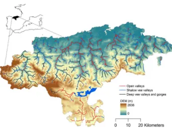
This study was developed in river catchments from the Cantabrian region, northern Spain (Fig. 1). Cantabrian rivers have their source in the Cantabrian Cordillera, a mountain range that runs parallel to the Atlantic Ocean coast and reaches up to 2600 m a.s.l. In the northern part of the re-gion, rivers drain into the Atlantic Ocean. These rivers are short, with high slopes and high erosive power. The largest basins slightly exceed 1000 km2and 20 m3s−1of mean daily
flow, with highly variable valley widths that rarely exceed 1.5 km in most of the middle and upper courses. This area has a humid oceanic temperate climate (Rivas-Mart´ınez et al., 2004) with an average annual temperature of 14◦C and
an average annual precipitation of 1200 mm. The southern part of Cantabria is dominated by a continental climate with an average annual temperature of 10◦
Fig. 1.River network of the Cantabrian region, northern Spain, and spatial distribution of the three considered valley types over the study area.
up to 700 m and by sub-Mediterranean alder groves (Alnus glutinosa) in the southern draining catchments (Lara et al., 2004). Willow groves formed bySalix atrocinerea (north-ern Cantabrian Cordillera) and Salix cantabrica (southern Cantabrian Cordillera) replace alder groves when they de-teriorate; soils are not deep enough or there are large flow fluctuations. Higher in altitude, ashes (Fraxinus excelsior) or hazelnuts (Corylus avellana) might dominate riparian forest, while in steep valleys beech, oak and mixed Atlantic for-est predominate. Finally, when riparian forfor-ests are impaired by human activities, the riparian vegetation is usually domi-nated byRubussp.,Rosasp.,Crataegus monogyna, Prunus spinosaor even pasture formations. For a more detailed de-scription of the study area, see Barqu´ın et al. (2012).
3 Methods
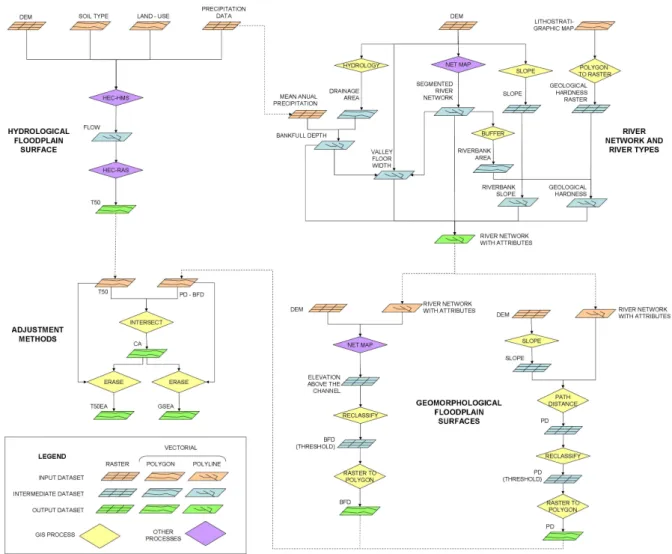
The methods used in the present work (Fig. 2) are orga-nized as follows. First we describe how we obtained the hydrological (Sect. 3.1) and geomorphological (Sect. 3.2) floodplain surfaces. Then we introduce the framework used for evaluating the adjustment (Sect. 3.3) and the two differ-ent adjustmdiffer-ent methods (Sect. 3.4). Finally, we explain how we accounted for the influence of DEM spatial resolution (Sect. 3.5).
3.1 Hydrological floodplain surface
The 50-yr flood has been indicated as an appropriate hydro-logical descriptor for riparian zones as it usually coincides with the first terrace or other upward sloping surface (Ilhardt et al., 2000). Moving outward this topographic boundary necessarily increases water table depth, and the probability of finding vegetation species related to riparian ecosystems may rapidly decrease. Therefore, 50-yr flood was selected in
the present study as the surface representing potential ripar-ian zone.
The area flooded by the 50-yr flood was available from a previous flood risk assessment study in the study area (IH Cantabria, 2008). In this study hydrological modelling with HEC MHS (US Army Corps of Engineers, 2000) was used to derive flow data. A high-resolution DEM (5-m spatial resolution, 1-m vertical accuracy), long series of precipita-tion data (more than 30 yr) and informaprecipita-tion about land-use and soil type (1 : 50 000 scale) were used as model inputs. For each river basin, flow was calculated at several points that were representative of homogeneous sub-basins. On the other hand, river hydraulics modelling was performed with RAS (US Army Corps of Engineers, 2005) and HEC-Geo RAS module, using the DEM to derive required cross-section data. This model required as input several parameters influencing flow behaviour: Manning’s number (in this study the authors used 0.04 for the channel and 0.06 for flood-plains, although variations were introduced where more de-tailed information was available), coefficients of expansion (0.3) and contraction (0.1) and boundary conditions (the wa-ter level at the river mouth cross-section was that of the high-est equinoctial tide).
3.2 Geomorphological floodplain surfaces
We used two different GIS-based geomorphologic ap-proaches to generate geomorphological floodplain surfaces. We referred to the first one as bankfull depth (BFD) ap-proach. BFD is the vertical distance from the deepest part of a channel to the bankfull elevation (Fig. 3), being the bank-full discharge the flow that fills a stream channel to the ele-vation of the active floodplain (Wolman and Leopold, 1957). Hence, BFD approach consists in generating a surface which intersects valley walls at a given number of BFD above the channel. We referred to the second method as the path tance (PD) approach. PD is the least accumulative cost dis-tance to the river channel when accounting for slope and el-evation change, indicating the relative costs of moving from the stream cells up into the stream valley. The PD approach uses a raster showing the PD value for each cell to gener-ate a surface covering all the locations along a river network which are encompassed by a certain path distance to the river channel. Both BFD and PD approaches require a DEM and a stream line as inputs to generate the floodplain surfaces. Ad-ditionally, BFD approach also requires BFD values in each segment of the river network. Before describing BFD and PD approaches, we described how we obtained the river network and BFD values.
3.2.1 River network and BFD values
Fig. 2.Flowchart illustrating the methods used to delineate the hydrological and geomorphological floodplain surfaces and the GIS processes used to obtain coinciding and exceeding areas.
Fig. 3.Floodplain cross-section defining the geomorphological pa-rameters in which the BFD approach relies on.
al. (2011). Hence, the network was delineated using flow di-rections inferred from a high-resolution DEM (5-m spatial resolution, 1-m vertical accuracy), using the algorithms de-scribed by Clarke et al. (2008). In flat areas, DEMs usually contain cells that are completely surrounded by other cells at the same or higher elevation. These cells act as sinks to over-land flow when deriving a river network using flow direction,
and different approaches exist to deal with this issue (e.g. Martz and Garbrecht, 1998; Lindsay and Creed, 2005; Nardi et al., 2008). In this study, we enforced drainage in low re-lief areas (slope less than 30 %) by lowering two meters the elevation of stream cells in the DEM using GIS data on chan-nel real locations. Then the chanchan-nel network was divided into channel segments (500–1000 m) and split at confluences, as they are supposed to produce changes in channel and flood-plain morphologies (Benda et al., 2004). This resulted in river reach longitudes ranging from 3 to 850 m (Fig. 4a).
Bankfull depth (BFD) was estimated for each river seg-ment using a regional regression of drainage area (A) and mean annual precipitation (P )to field measured depths over a range of channel sizes encompassing 195 river sites in the region of Cantabria (selected in areas with little to no engi-neered works). The results of this analysis yielded the fol-lowing equation (Eq. 1):
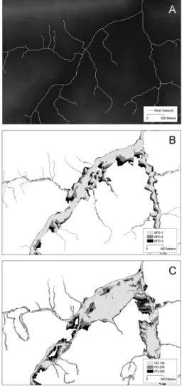
Fig. 4.Illustration of river centre-lines over the digital elevation model at a confluence (A) and bankfull depth floodplain surfaces (B; at 1, 2 and 3 bankfull depth heights) and path distance flood-plain surfaces (C; at 100, 200 and 300 threshold values) at the same location.
This model has been used in other recent applications (Benda et al., 2011), and it was the only one available at the time of pursuing this study for the Cantabrian region. However, it should be noted that BFD estimates might present deviations from observed values (p <0.001; R2=0.12), as BFD is highly sensible to local channel morphology and the present model only includes catchment area and mean annual precip-itation.
3.2.2 BFD approach
The area bordering a stream that will be covered by water at a flood stage of twice the maximum BFD is called the flood-prone area and corresponds on average to that which becomes flooded by the 50-yr flood (Rosgen, 1996). How-ever, flood-prone height ranges from 1.3 times the BFD in rivers of Rosgen’s type E (low-gradient meandering rivers)
to 2.7 times the BFD in rivers of type A (highly entrenched streams), and generally includes the active floodplain and the low terrace (Rosgen, 1996). Based on Rosgen’s empirical data, valley width at a height of approximately 2 times the BFD must coincide with the surface flooded by 50-yr flood. However, this relationship may be different when modelling in a GIS environment. Hence, we derived several geomor-phologic floodplain surfaces using different bankfull depth heights (Fig. 4b) ranging from 0.25 to 3 using steps of 0.25.
To that end we used NetMap tools to transform the DEM (we used a 10-m DEM instead of the 5-m DEM due to com-putational limitations) into a raster where each cell was asso-ciated with the closest river segment (in Euclidean distance) presenting the fewest and smallest intervening high points. Cell values showed then the elevation difference (in terms of BFD) among the cell and its associated channel. Using this raster, it was possible to assess valley width at an elevation equivalent to a given number of BFDs for each river segment, and therefore generate geomorphological floodplain surfaces (polygon shapefile format) using the range of BFDs cited above. Hereafter we will refer to these surfaces as BFD-X, being X the factor multiplying bankfull depth (e.g. BFD-1.25).
3.2.3 PD approach
A PD raster was derived using the PD tool in ArcGIS soft-ware (ESRI, 2011). PD tool required the following inputs: the river network (polyline shapefile) to identify stream cells, a DEM (a 10-m DEM, in order to be comparable with the sur-faces generated by the BFD approach) as a surface raster and a slope raster as a cost layer. Then we used the reclassify tool to derive several surfaces (polygon shapefiles; Fig. 4c) cor-responding with path distance threshold values ranging from 50 to 350 m using steps of 50 m. This range was determined by querying the values of several cells in the PD raster lo-cated at the edge of the 50-yr flood in different valley mor-phologies. Hereafter we will refer to the generated surfaces as PD-Y, beingY the threshold value used to generate that surface (e.g. PD-250).
3.3 Framework for evaluating the adjustment
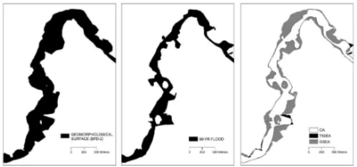
Fig. 5.Delineation of coinciding area (CA), 50-yr flood exceed-ing area (T50EA) and geomorphological surface exceedexceed-ing area (GSEA) to evaluate the adjustment between geomorphological (BFD-2) and hydrological criteria (50-yr flood) derived surfaces.
3.3.1 River types
The geomorphological attributes used to define river types were channel and riverbank slope (considering as river-bank zone a buffer of 200 m from the river channel), val-ley floor width and riverbank geological hardness. These four attributes are related to the flood height at a given location. Thus, channel slope is important to distinguish among high-energy straight rivers and low-energy meander-ing rivers. Both riverbank slope and valley floor width char-acterise cross-section topography for each river reach. And last, riverbank geological hardness differentiates those loca-tions where river flows across alluvial, easily erodible mate-rial from those flowing across hard, difficultly erodible geo-logical substrate. Valley floor width is difficult to define for some valley morphologies, especially in V-shaped valleys. Generally, the edge of the valley floor is located in the first terrace or other major sloping surface, which usually corre-sponds with the 50-yr flood (Ilhardt et al., 2000). At the same time and as cited above, 50-yr flood corresponds on average to a flood stage of twice the maximum BFD (Rosgen, 1996). Hence, we used valley width at a height of two times the BFD as an approximation of the real valley width.
Channel slope and riverbank slope were calculated at the endpoint of each segment from the DEM. Valley floor width was obtained from BFD-2 surface, derived as described in Sect. 3.2.2. Riverbank geological hardness was derived from the Spanish lithostratigraphic map (source: Geological and Mining Institute of Spain; spatial scale: 1 : 200 000). To that end we reclassified original geological classes into broader ones and then we assigned them a numerical value based on geological hardness (see Snelder et al., 2008, for de-tails). This map was then converted into a raster layer. Finally we obtained riverbank hardness for each river reach using NetMap tools.
The four geomorphological attributes were finally used to classify the river network in geomorphological types by us-ing PAM (partition around medoids) clusterus-ing in R soft-ware (R Development Core Team, 2008), previous data
Fig. 6.Boxplots of the four variables involved in the river reach classification for the three geomorphological valley types.
standardization. PAM clustering was performed using differ-ent pre-established numbers of clusters (3, 4 and 5). Then, we analysed the characteristics of each cluster (geomorphologi-cal type) with respect to the four geomorphologi(geomorphologi-cal attributes using boxplots.
3.3.2 River network pruning
The 50-yr flood was not available for headwaters (Strahler order 1 and 2). From the 427 km where this information was available, we discarded those river segments presenting sig-nificant flood restrictions. We considered as sigsig-nificant re-strictions all bank reinforcements or embankments longer than 100 m. We also excluded river reaches located down-stream from dams. The remaining river network comprised 321 km of rivers.
3.4 Adjustment methods
First, each geomorphological surface was divided based on river types and the total area in each type was calculated. Then we evaluated the adjustment of each surface with re-spect to the 50-yr flood using two different methods:
i. Minimum exceeding score (Eq. 2). This method com-bines the two possible exceeding surfaces: geomorpho-logical surface exceeding area (GSEA) and 50-yr flood exceeding area (T50EA; Fig. 5). GSEA is the area of the geomorphological surface exceeding the 50-yr flood, while the T50EA is the area of the 50-yr flood not covered by the geomorphological surface. This latter parameter results from subtracting the coinciding area (CA; Fig. 5) from the 50-yr flood. Both GSEA and T50EA are expressed as a percentage with respect to the area occupied by the 50-yr flood. The optimal geomor-phological surface is that achieving the lowest minimum exceeding score.
Fig. 7.Adjustment parameters when using a 10-m DEM: coinciding area (CA), 50-yr flood exceeding area (T50EA) and geomorpholog-ical surface exceeding area (GSEA) for bankfull depth (1,3and5) and path distance (2,4and6) approaches in open valleys (A), shal-low vee valleys (B) and deep vee valleys (C).
ii. Total area (Eq. 3). This method does not look at coin-ciding or exceeding areas, but only considers the de-viance between the value of the area occupied by the geomorphological surface and the value of the area cov-ered by the 50-yr flood. Total area optimum value is 100, and values above or below are considered as de-viations. This condition may not reflect an “optimum adjustment”, but, as all geomorphological surfaces and the 50-yr flood are supposed to be sensitive to geomor-phology, we considered exploring this possibility.
Total area=geomorphological surface total area
area covered by the 50-yr flood ×100 (3)
3.5 Influence of DEM spatial resolution
As the DEM is the main input in our geomorphological ap-proaches, we wanted to test the influence of DEM spatial resolution in the performance of the present methodology. To that end, we have derived again all the geomorphologic floodplain surfaces under the BFD and PD approaches using a 30-m DEM, and compared their adjustment with the 50-yr flood as described in Sect. 3.4.
Fig. 8.Adjustment parameters when using a 30-m DEM: coinciding area (CA), 50-yr flood exceeding area (T50EA) and geomorpholog-ical surface exceeding area (GSEA) for bankfull depth (1,3and5) and path distance (2,4and6) approaches in open valleys (A), shal-low vee valleys (B) and deep vee valleys (C).
4 Results
Cluster analysis showed that increasing the number of clus-ters (from 3 to 5) did not produce an increase in classification strength (not shown). Hence, we chose three groups (clus-ters) to gain in simplicity and because the resulting groups highly reflect valley morphologies in our study area (see Fig. 1). The first of these groups included 1782 cases and corresponded with open valleys, as it presented the widest valleys (average >200 m), the lowest geological hardness and the lowest channel and stream bank slopes (average of 6 degrees and 13 %, respectively; Fig. 6). The second one encompassed 1953 cases and corresponded with shallow-vee valleys presenting intermediate characteristics between the other two groups. Finally, the third group included 1908 cases and corresponded with deep-vee valleys and gorges, as it showed narrower valley widths (average<50 m), high ge-ological hardness and the steepest channel and stream bank slopes (average of 22 degrees and 50 %, respectively).
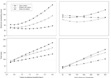
Fig. 9.Values obtained for the two different methods used to evalu-ate the adjustment between geomorphological surfaces and the 50-yr flood when using a 10-m DEM. Arrows indicate optimal thresh-old values (best adjustment) for each geomorphological approach and valley type.
When using the 10-m DEM the adjustment between geo-morphological and hydrological floodplain surfaces, in terms of coinciding and exceeding areas, showed the same general trend for all river types and the two geomorphological ap-proaches (Fig. 7). As it was expected, increasing the geo-morphological surface (by increasing the factor multiplying BFD or increasing the PD threshold value) increased CA, and therefore decreased T50EA. However, increasing the ge-omorphological surface also increased GSEA. Besides, the rate of increase of GSEA was greater than that of CA, except in deep-vee valleys, where they presented almost the same rate. Intersection between T50EA and GSEA showed the op-timal multiplying factor for the geomorphological surface with respect to the 50-yr flood. This intersection occurred at larger geomorphological surfaces when moving from open valleys to more entrenched ones, although there were no dif-ferences between open and shallow vee valleys. Despite the homogeneity in the above cited trends, the BFD approach reaches higher CA values than path distance. Consequently, PD reached higher T50EA values than BFD approach. How-ever, both approaches showed similar values for GSEA. All these general trends cited above also occurred in open and shallow-vee valleys when using a 30-m DEM (Fig. 8). Coin-ciding and exceeding areas were also similar (except for PD approach when using low PD values), although the intersec-tion of T50EA and GSEA occurred at lower threshold values (except for BFD approach in open valleys). Regarding deep-vee valleys, 30-m DEM produced almost the similar surface for all the range of thresholds used in both approaches (so CA, GSEA and T50EA followed a nearly horizontal line in Fig. 8, and intersection between T50EA and GSEA never oc-curred). Besides, for PD approach GSEA was always higher than CA.
Fig. 10.Adjustment between the 50-yr flood and the optimal geo-morphological floodplain surfaces for bankfull depth (1, 3 and 5) and path distance (2, 4 and 6) approaches in open valleys (A), shal-low vee valleys (B) and deep vee valleys (C).
Total area method for evaluating the adjustment between the hydrological and geomorphological floodplain surfaces pointed out the same optimum threshold as the graphical in-tersection of GSEA and T50EA for both BFD and PD ap-proaches (Fig. 9; only 10-m DEM adjustment is presented, as similar patterns are found for open and shallow vee valleys when working with a 30-m DEM). When using minimum ex-ceeding score, only BFD complied with this statement. The total area method showed a positive linear relationship be-tween the value defining the geomorphological surface and its total area. The slope of this relationship became steeper when moving from deep vee to open valleys. The BFD value that best matched the 50-yr flood was BFD-0.5 in open and shallow vee valleys and 1.25 in deep vee valleys. For PD ap-proach, optimal adjustment occurred at PD-200 in open and shallow vee valleys and PD-350 in deep vee valleys. The ad-justment of optimal geomorphological surfaces with respect to the 50-yr flood is shown in Fig. 10.
5 Discussion and conclusion
Fig. 11. Illustration of the flood-prone area at 1.25-BFD over the digital elevation model: at a river confluence deriving in wider flood-prone areas (A), at a river confluence not deriving in wider flood-prone areas (B) and at an unconstrained-constrained-unconstrained valley transition (C).
(i) sensitivity to topography, (ii) few inputs required and (iii) possibility of covering large areas. Hence, they consti-tute a remarkable improvement with respect to fixed buffer approaches and provide useful information for management in areas lacking hydrological data. They are, however, still not suitable for purposes requiring highly accurate data, such as flood damage prevention. Our methodology was strength-ened by taking into account the influence of the following parameters: geomorphological approach, valley type, adjust-ment method and DEM spatial resolution. All of these pa-rameters are discussed below.
Regarding geomorphological approach performance, both BFD and PD showed sensitivity to floodplain morphol-ogy and seemed valid to delineate riparian areas. BFD ap-proach performance is better as the resulting geomorpho-logical floodplain surfaces correspond with higher CA (10– 19 % depending on valley type) and lower GSEA (12–24 %)
and T50EA (10–19 %) than those for PD when using a 10-m DEM (larger differences a10-mong perfor10-mance correspond with deep vee valleys). These differences among both ap-proaches are reduced by two-thirds when using a 30-m DEM, although BFD approach performed better than PD also at this resolution. On the other hand, PD approach does not require BFD values for each river reach in the network and it can be rapidly calculated in GIS. Moreover, the quality of the BFD regional model is important when there are not hydrological surfaces that could be used to match with the BFD estimated surfaces. In our model, BFD values were oversized, so we obtained optimal adjustment with the hydrological floodplain at lower values than those obtained by Rosgen (1996). To sum up, the choice of the proper geomorphological method depends on the resources and accuracy required. Besides, both BFD and PD approaches present the advantage of be-ing suitable to account for the gradients present in riparian zones by assigning “membership to riparian zones” scores to each band defined by a different threshold value (the lesser the threshold value is, the higher must be the membership score as the river influence is also higher).
Despite of differing in characteristics as streamside slope or valley width, there is no need of distinguishing between open and shallow vee valleys (as defined in this study) when using our geomorphologic approaches to delineate riparian areas, as the same optimal geomorphological floodplain sur-face is obtained for both valley types. However, deep vee valley and gorges (constrained river reaches) require higher BFD values than unconstrained rivers to match with the 50-yr flood, as described also by Rosgen (1996). Hence, at least these two categories (constrained-unconstrained) should be taken into account. Besides, the lesser the degree of con-strainment is, the worse is the adjustment in terms of GSEA. Similar results were obtained by Sutula et al. (2006). This may be due to the fact that unconstrained valleys present more complex fluvial landscapes than constrained ones. We have also considered that tributary confluences may also partly explain the disarrangement between geomorphologi-cal surfaces and the 50-yr flood, as they have not been con-sidered in defining river types. In general terms they result in lower channel gradients and wider channel and floodplains (Benda et al., 2004; Fig. 11a). However, topographic con-strains such as steep riverbank slopes or hardly erodible river-bank materials seemed to be more determinant of floodplain width than confluence effects at some large channel conflu-ences in our study area (e.g., Fig. 11b, where the main chan-nel is the Deva River, and Quiviesa and Bull´on are large trib-utaries). Hence, it does not seem appropriate to include a variable accounting for confluence effects when classifying valley type, at least in mountainous study areas such as in here. In addition, we do find larger fluvial landscapes imme-diately above and below valley constrictions (Fig. 11c), as commented in Benda et al. (2011).
close to the optimum. By looking at total area, it can be seen that this is not true, as moving backward or forward the op-timum value significantly causes rapid deviation from 100 % of total area, and this is reflected in exceeding and coinciding area combinations away from the optimum.
Results were dependant on DEM spatial resolution, as suggested in other studies dealing with riparian delineation (Nardi et al., 2006; Sutula et al., 2006; Abood and Maclean, 2011). In our study area, 10-m and 30-m DEM resulted in similar adjustment in open and shallow vee valleys, regard-less of the geomorphological approach used. 30-m DEM, however, proved to be an unsuitable input for delineating ri-parian zones in deep vee valleys, as its resolution was not able to properly detect the valley cross-section morphology. Accordingly, the minimum DEM spatial resolution to be used depends on river and valley dimensions. Based on the differences between 10-m and 30-m DEM performance, sig-nificant improvement is expected when using higher spatial resolutions (e.g. 5 m), especially when using PD-approach.
In conclusion, our results suggest that using GIS to delin-eate sensitive-to-geomorphology, hydrologically meaning-ful, riparian zones is feasible and relatively easy and fast. However, this task requires local calibration in order to find an optimal threshold value for the geomorphological ap-proach which maximizes the coinciding and minimizes the exceeding with respect to the hydrological surface. Our re-sults also suggest that this optimal threshold value depends on valley morphology (constrained valleys require higher values unconstrained ones) and DEM spatial resolution.
Acknowledgements. We would like to thank to Lee Benda and Daniel Miller (Earth Systems Institute, CA, USA) for their col-laboration and support at different stages of this research. We also thank Fernando Nardi, Nicola Clerici and an anonymous referee for their valuable comments to the manuscript. Finally, we thank Ben P. Gouldby for the linguistic revision of the manuscript. This study was partly funded by the Spanish Ministry of Science and Innovation as part of the project MARCE (Ref: CTM-2009-07447) and by the Program of Postdoctoral Fellowships for Research Activities of the University of Cantabria (published by resolution on 17 January 2011).
Edited by: P. Passalacqua
Barqu´ın, J., Ondiviela, B., Recio, M., ´Alvarez-Cabria, M., Pe˜nas, F. J., Fern´andez, D., G´omez, A., ´Alvarez C., and Juanes, J. A.: Assessing the conservation status of alder-ash alluvial forest and Atlantic salmon in the Natura 2000 river network of Cantabria, Northern Spain, in: River Conservation and Management: 20 years on, edited by: Boon, P. J. and Raven, D. P. J., Wiley-Blackwell, Chichester, West Sussex, UK, 2012.
Benda, L., Poff, N. L., Miller, D., Dunne, T., Reeves, G., Pess, G., and Pollock, M.: The network dynamics hypothesis: how channel networks structure riverine habitats, Bioscience, 54, 413–427, 2004.
Benda, L., Miller, D., Andras, K., Bigelow, P., Reeves, G., and Michael, D.: NetMap: a new tool in support of watershed science and resource management, Forest Sci., 53, 206–219, 2007. Benda, L., Miller, D., Lanigan, S., and Reeves, G.: Future of applied
watershed science at regional scales, EOS T. Am. Geophys. Un., 90, p. 156, doi:10.1029/2009EO180005, 2009.
Benda, L., Miller, D., and Barqu´ın, J.: Creating a catchment scale perspective for river restoration, Hydrol. Earth Syst. Sci., 15, 2995–3015, doi:10.5194/hess-15-2995-2011, 2011.
Bhowmik, N. G.: Hydraulic geometry of floodplains, J. Hydrol., 68, 369–374, 1984.
Clarke, S. E., Burnett, K. M., and Miller, D. J.: Modeling streams and hydrogeomorphic attributes in Oregon from digital and field data, J. Am. Water Resour. As., 44, 459–477, 2008.
Clerici, N., Weissteiner, C. J., Paracchini, M. L., and Strobl, P.: Riparian zones: where green and blue networks meet. Pan-European zonation modelling based on remote sensing and GIS, Joint Research Centre of the European Comission, Luxembourg, Technical Report, 60 pp., 2011.
Clerici, N., Weissteiner, C. J., Paracchini, M. L., Boschetti, L., Baraldi, A., and Strobl, P.: Pan-European distribution modelling of stream riparian zones based on multi-source Earth Observa-tion data, Ecol. Indic., 24, 211–223, 2013.
Dodov, B. and Foufoula-Georgiou, E.: Generalized hydraulic geom-etry: Derivation based on multiscaling formalism, Water Resour. Res., 40, W06302, doi:10.1029/2003WR002082, 2004. Dodov, B. and Foufoula-Georgiou, E.: Floodplain Morphometry
Extraction From a High-Resolution Digital Elevation Model: A Simple Algorithm for Regional Analysis Studies, IEEE Geosci. Remote S., 3, 410–413, doi:10.1109/LGRS.2006.874161, 2006. Environmental Systems Research Institute (ESRI): ArcGIS Desk-top: Release 10, Environmental Systems Research Institute, Red-lands, CA, USA, 2011.
Gregory, S. V., Swanson, F. J., McKee, W. A., and Cummins, K. W.: An ecosystem perspective of riparian zones, Bioscience, 41, 540–551, 1991.
Hruby, T.: Developing rapid methods for analyzing upland riparian functions and values, Environ. Manage., 43, 1219–1243, 2009. Hupp, C. R. and Osterkamp, W. R.: Riparian vegetation and fluvial
geomorphic processes, Geomorphology, 14, 277–295, 1996. IH Cantabria: Desarrollo de la documentaci´on t´ecnica y cartogr´afica
para la redacci´on del plan de protecci´on civil ante el riesgo de in-undaciones de la Comunidad Aut´onoma de Cantabria, Direcci´on General de Protecci´on Civil, Consejer´ıa de Presidencia, Gob-ierno de Cantabria, Santander, Spain, Technical Report, 12 pp., 2008.
Ilhardt, B. L., Verry, E. S., and Palik, P. J.: Defining riparian ar-eas, in: Riparian Management in Forests of the Continental East-ern United States, edited by: Verry, E. S., Hornbeck, J. W., and Dollof, C. A., Lewis Publishers, Boca Raton, Florida, USA, 2000.
Lara, F., Garilleti, R., and Calleja, J. A.: La vegetaci´on de ribera de la mitad norte Espa˜nola, Monografias, 81, p. 536, 2004. Lindsay, J. B. and Creed, I. F.: Removal of artefact depressions from
digital elevation models: towards a minimum impact approach, Hydrol. Process., 19, 3113–3126, 2005.
Mac Nally, R., Molyneux, G., Thomson, J. R., Lake, P. S., and Read, J.: Variation in widths of riparian-zone vegetation of higher-elevation streams and implications for conservation manage-ment, Plant Ecol., 198, 89–100, 2008.
Martz, L. W. and Garbrecht, J.: The treatment of flat areas and de-pressions in automated drainage analysis of raster digital eleva-tion models, Hydrol. Process., 12, 843–855, 1998.
McGlynn, B. L. and Seibert, J.: Distributed assessment of contribut-ing area and riparian buffercontribut-ing along stream networks, Water Re-sour. Res., 39, 1082, doi:10.1029/2002WR001521, 2003. Merritt, D. M., Scott, M. L., Poff, N. L., Auble, G. T., and Lytle,
D. A.: Theory, methods and tools for determining environmental flows for riparian vegetation: riparian vegetation-flow response guilds, Freshwater Biol., 55, 206–225, 2009.
Naiman, R. J., D´ecamps, H., and Pollock, M.: The role of ripar-ian corridors in maintaining regional biodiversity, Ecol. Appl., 3, 209–212, 1993.
Naiman, R. J., D´ecamps, H., and McClain, M.: Riparia: Ecology, Conservation, and Management of Streamside Communities, El-sevier Academic Press, 448 pp., San Diego, California, USA, 2005.
Nardi, F., Vivoni, E. R., and Grimaldi, S.: Investigating a floodplain scaling relation using a hydrogeomorphic delineation method, Water Resour. Res., 42, W09409, doi:10.1029/2005WR004155, 2006.
Nardi, F., Grimaldi, S., Petroselli, A., Santini, M., and Uber-tini, L.: Hydrogeomorphic properties of simulated drainage pat-terns using DEMs: the flat area issue, Hydrolog. Sci. J., 53, doi:10.1623/hysj.53.6.1176, 2008.
National Research Council (NRC), Committee on Riparian Zone Functioning and Strategies for Management: Riparian areas: functions and strategies for management, National Academy Press, Washington, DC, USA, 444 pp., 2002.
Naura, M., Sear, D., ´Alvarez-Cabria, M., Pe˜nas, F. J., Fern´andez, D., and Barqu´ın, J.: Integrating monitoring, expert knowledge and habitat management within conservation organisations for the delivery of the water framework directive: a proposed ap-proach, Limnetica, 30, 427–446, 2011.
Noman, N. S., Nelson, E. J., and Zundel, A. K.: Review of auto-mated floodplain delineation from digital terrain models, J. Water Res. Pl.-ASCE, 127, 394–402, 2001.
Osterkamp, W. R. and Hupp, C. R.: Fluvial processes and vegeta-tion – glimpses of the past, the present, and perhaps the future, Geomorphology, 116, 274–285, 2010.
Palik, B. J., Tang, S. M., and Chavez, Q.: Estimating riparian area extent and land use in the Midwest, Gen. Tech. Rep. NC-248., Department of Agriculture, Forest Service, North Central Re-search Station, St. Paul, MN, 28 pp., 2004.
Perkins, D. W. and Hunter, M. L.: Use of amphibians to define ri-parian zones along headwater streams in Maine, Can. J. Forest Res., 36, 2124–2130, 2006.
Poff, B., Koestner, K. A., Neary, D. G., and Henderson, V.: Threats to riparian ecosystems in Western North America: an analysis of existing literature, J. Am. Water Resour. As., 47, 1241–1254, 2011.
Poole, G. C.: Fluvial landscape ecology: addressing uniqueness within the river discontinuum, Freshwater Biol., 47, 641–660, 2002.
R Development Core Team: A language and environment for statis-tical computing, Vienna, Austria, software 3-900051-07-0, 2008. Rivas-Mart´ınez, S., Penas, A., and D´ıaz, T. E.: Bioclimatic Map of Europe, in: Bioclimates, Le´on University, Cartographic Service, Le´on, Spain, 2004.
Rosgen, D. L.: Applied river morphology, Wildland Hydrology, Pagosa Springs, CO, USA, 1996.
Snelder, T., Pella, H., Wasson, J.-G., and Lamouroux, N.: Defini-tion procedures have little effect on performance of environmen-tal classifications of streams and rivers, Environ. Manage., 42, 771–788, 2008.
Staats, J. and Holtzman, S.: Keeping water on the land longer – Healthy streams through bringing people together, University of California Water Resources Center, Stevenson, WA, USA, 2002. Sutula, M., Stein, E. D., and Inlander, E.: Evaluation of a method to cost-effectively map riparian areas in Southern California coastal watersheds, Technical Report 480, Southern California Coastal Water Research Project (SCCWRP), 2006.
Tabacchi, E., Correll, D. L., Hauer, R., Pinay, G., Planty-Tabacchi, A. M., and Wissmar, R. C.: Development, maintenance and role of riparian vegetation in the river landscape, Freshwater Biol., 40, 497–516, 1998.
Thorp, J. H., Thoms, M. C., and Delong, M. D.: The riverine ecosys-tem synthesis: biocomplexity in river networks across space and time, River Res. Appl., 22, 123–147, 2006.
US Army Corps of Engineers: Hydrologic Modeling System HEC-HMS, Technical Reference Manual, Hydrologic Engineering Center, Davis, CA, USA, 155 pp., 2000.
US Army Corps of Engineers: HEC-RAS river analysis system, Hy-draulic Reference Manual ver. 3.1.3, 262 pp., Hydrologic Engi-neering Center, Davis, CA, USA, 2005.
US Department of Agriculture Forest Service (USDA FS): Water-shed Protection and Management, Forest Service Manual Chap-ter 2520, 26 pp., 1994.