Res. Biomed. Eng. vol.32 número3

DOI: http://dx.doi.org/10.1590/2446-4740.04915

*e-mail: cffcilho@gmail.com

Received: 09 December 2013 / Accepted: 13 September 2016

Breast tumor classiication in ultrasound images using support

vector machines and neural networks

Carmina Dessana Lima Nascimento, Sérgio Deodoro de Souza Silva, Thales Araújo da Silva, Wagner Coelho de Albuquerque Pereira, Marly Guimarães Fernandes Costa, Cicero Ferreira Fernandes Costa Filho*

AbstractIntroduction: The use of tools for computer-aided diagnosis (CAD) has been proposed for detection and classiication of breast cancer. Concerning breast cancer image diagnosing with ultrasound, some results found in literature show that morphological features perform better than texture features for lesions differentiation, and indicate that a reduced set of features performs better than a larger one. Methods: This study evaluated the performance of support vector machines (SVM) with different kernels combinations, and neural networks with different stop criteria, for classifying breast cancer nodules. Twenty-two morphological features from the contour of 100 BUS images were used as input for classiiers and then a scalar feature selection technique with correlation was used to reduce the features dataset. Results: The best results obtained for accuracy and area under ROC curve were 96.98% and 0.980, respectively, both with neural networks using the whole set of features. Conclusion: The performance obtained with neural networks with the selected stop criterion was better than the ones obtained with SVM. Whilst using neural networks the results were better with all 22 features, SVM classiiers performed better with a reduced set of 6 features.

Keywords: Breast tumors, Breast ultrasound images, Neural network, Support vector machine.

Introduction

Breast cancer remains the leading cause of death among women in developed and developing countries. It is the most common cancer in women worldwide representing about 12% of all new cases and 25% of all cancers in women (World…, 2014). In Brazil, it ranks irst in incidence in the Northeast, South and Southwest, in proportion 22.84%, 24.14% and 23.83% respectively. In North and Midwest, this incidence is second only to cervical cancer (Sociedade…, 2015).

In the world population, survival rate ive years after diagnosis is 61%, however in Brazil breast cancer mortality rate remains high, mainly because in most cases the disease is diagnosed in advanced stages (Instituto…, 2015).

Early detection is the main strategy for breast cancer prevention and control. However, early detection requires an accurate and reliable diagnosis. A good detection approach should produce both low false positive (FP) rate and false negative (FN) rate (Cheng et al., 2010).

Due to its high resolution that enables nodule detection, a mammographic exam is one of the most important tools used for breast cancer screening. Typically, breast cancer appears in mammographic

images as microcalciication clusters with irregular shapes. Microcalciications are small calcium deposits inside breast tissue that sometimes are associated with active processes of tumor cells (Kramer and

Aghdasi, 1999).

Mammography remains the procedure of choice in screening asymptomatic women for breast cancer, and has a major impact on the effectiveness of therapy. However, a large number of doubtful solid masses are usually forwarded to surgical biopsy, an invasive and painful procedure, although only 10-30% of them are malignant. This restriction increases the cost and stress imposed on the patient (Dennis et al., 2001).

With the aim to increase speciicity of breast cancer image diagnostics, breast ultrasound (BUS) emerged as an important complement to mammography. Ultrasound is more sensitive for detecting invasive cancer in dense breasts (Skaane, 1999). However, it is an operator-dependent modality, and the interpretation of its images requires expertise from the radiologist.

To minimize operator dependency and improve the diagnostic accuracy, computer-aided diagnosis (CAD) systems has been proposed to detect and classify breast cancer nodules (Uniyal et al., 2013).

CAD systems provide important information based on computer analysis of the BUS images assisting health professionals to locate lesions and classify them as benign or malignant.

Regarding lesions in BUS images, literature shows that features related to morphology and texture are used for differentiating between malignant and benign lesions. Flores et al. (2015), in a literature review, listed 26 morphological features and 1465 texture features used for this task.

Some results found in the literature show a better performance of morphological features in breast cancer lesion differentiating. Alvarenga et al. (2007) obtained a poorer performance with texture features than with a morphological feature set (Alvarenga et al., 2010), using a Fisher linear discriminant ratio classiier. With a combined set of features, the same authors did not surpass the previous results obtained with the morphological feature set.

With the purpose of inding the smallest set of morphological features producing an effective improvement in classiication performance, Flores et al. (2015) evaluated a set of morphological and textural features proposed in the literature. As a result, the

authors suggest using only ive morphological features to classify breast lesions.

The most commonly used pattern recognition classiiers employed for breast cancer detection in BUS images are: neural networks (Alvarenga et al., 2005; Chen et al., 1999; 2003), stepwise logical regression (Chiang et al., 2001), support vector machines (Huang et al., 2008;

Renjie et al., 2011; Wu and Moon, 2008), Fisher linear

discriminant ratio (Alvarenga et al., 2012; Flores et al.,

2015), and decisions trees (Kuo et al., 2001). In this paper, we aim to investigate the results of new methods for improving neural network generalization and the results of SVM classiiers with different kernels over the classiication performance of breast cancer lesions in ultrasound images. Using the set of features compiled by Flores et al. (2015), we also tested the effect of dimensionality reduction of the input data on both neural network and SVM performance, using scalar feature ranking with a correlation technique. For training and testing the classiiers, the 4-fold-cross-validation method was used (Leisch et al., 1998).

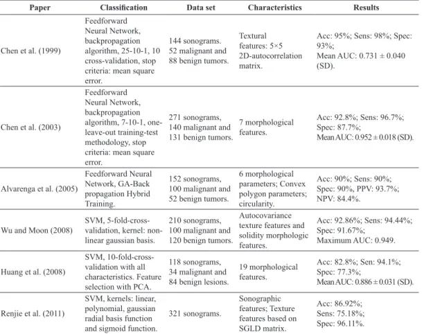
Table 1 shows characteristics of three published studies using a neural network and three published studies using SVM for breast cancer classiication.

Table 1. A brief review of breast cancer classiication using neural network and SVM.

Paper Classiication Data set Characteristics Results

Chen et al. (1999)

Feedforward Neural Network, backpropagation algorithm, 25-10-1, 10 cross-validation, stop criteria: mean square error.

144 sonograms. 52 malignant and 88 benign tumors.

Textural features: 5×5 2D-autocorrelation matrix.

Acc: 95%; Sens: 98%; Spec: 93%;

Mean AUC: 0.731 ± 0.040 (SD).

Chen et al. (2003)

Feedforward Neural Network, backpropagation algorithm, 7-10-1, one-leave-out training-test methodology, stop criteria: mean square error.

271 sonograms, 140 malignant and 131 benign tumors.

7 morphological features.

Acc: 92.8%; Sens: 96.7%; Spec: 87.7%;

Mean AUC: 0.952 ± 0.018 (SD).

Alvarenga et al. (2005)

Feedforward Neural Network, GA-Back propagation Hybrid Training.

152 sonograms, 100 malignant and 52 benign tumors.

6 morphological parameters; Convex polygon parameters; circularity.

Acc: 90%; Sens: 90%; Spec: 90%, PPV: 93.7%; NPV: 84.4%.

Wu and Moon (2008) SVM, 5-fold-cross-validation, kernel: non-linear gaussian basis.

210 sonograms, 100 malignant and 120 benign tumors.

Autocovariance texture features and solidity morphologic features.

Acc: 92.86%; Sens: 94.44%; Spec: 91.67%;

Maximum AUC: 0.949.

Huang et al. (2008)

SVM, 10-fold-cross-validation with all characteristics. Feature selection with PCA.

118 sonograms, 34 malignant and 84 benign lesions.

19 morphological features.

Acc: 82.8%; Sen: 94.1%; Spec: 77.3%;

Mean AUC: 0.886 ± 0.031 (SD).

Renjie et al. (2011)

SVM, kernels: linear, polynomial, gaussian radial basis function and sigmoid function.

321 sonograms.

Sonographic features; Texture features based on SGLD matrix.

As shown, the accuracy in irst three studies varies between 90% and 95% and in the three last studies varies between 82% and 92%, suggesting a better performance of neural network classiiers over SVM classiiers.

Methods

The methodology for breast tumor classiication is comprised of the following steps: dataset acquisition, feature selection, dataset division and classiication. In the classiication step, two techniques were investigated: SVM and neural network classiiers. The scalar feature selection technique was used to identify the best characteristics. The methodological topics mentioned will be presented below.

Dataset acquisition

In this retrospective study, using a 7.5-MHz linear array B mode 40-mm ultrasound probe (Siemens Sonoline Sienna_{) with axial resolutions}

of 0.45 and 0.49mm respectively, 100 US breast tumor images were acquired from 100 patients of the National Cancer Institute (INCa, Rio de Janeiro, Brazil). It is worth clarifying that this study was carried out according to INCa’s diagnosis routine. Hence, the US images were obtained after patients’ clinical examination and mammography, and then it was decided whether the patient should be submitted to biopsy.

Only BUS images from patients with histopathological diagnosis were selected, resulting in an image set of 50 malignant and 50 benign tumors.

Figure 1 shows BUS image examples available on the dataset.

For each image, a rectangular ROI, including the tumor and its neighboring area was determined by a radiologist (a medical doctor with 30 years of experience in mammography and breast ultrasound interpretation). The radiologist was requested to select the portion of the image background surrounding the lesion that includes essential information for the routine sonographic diagnosis. Besides, each ROI was segmented using the semiautomatic contour (SAC) procedure, based on morphological operators (Alvarenga et al., 2012).

A set of 22 features, from each lesion was extracted. These features are divided into ive classes: one class related to morphological skeleton; one class related to radial normalized length; one class related to a lesion convex polygon; one class related to circularity and one class related to equivalent ellipse.

Two of them are related to morphological skeleton: elliptic normalized skeleton (ENS) and skeleton end (S#). Six of them are related to radial normalized

length (NRL): NRL area ratio (dA), NRL mean (dμ),

NRL standard deviation (dσ) , NRL entropy (dE),

NRL roughness (dR) and NRL crossing (dZ). Nine

of them are related to the lesion convex polygon: Overlap ratio (RS), Number of protuberances and depressions (NSPD), Lobulation index (LI), Normalized residual value (NRV), Proportional distance (PD), Convexity (Cnvx), Elliptic normalized circumference (ENC), Hausdorff distance (HD) and Average distance (MD). Four of them are related

to circularity: orientation (OE), Circularity A (Ca),

Circularity B (Cb) and Circularity C (Cc). One of them

is related to equivalent ellipse: Depth-to-width ratio (DWR). All of them are described in (Flores, 2009).

Feature selection

To identify the most important features to reduce the feature vector dimensionality while retaining as much as possible of their class discriminatory information and with the aim of evaluating the effect of a reduced set of variables on the classiication performance, the scalar selection technique with correlation was used (Theodoridis and Koutroumbas, 2008).

With the aim to select features leading to large between-class distance and small within-class variance in the feature vector space, the class separation measurement used in this study was Fisher’s Discriminant Ratio (FDR) described in Equation 1:

( )2

1 2

2 2

1 2

k k k

k k

FDR = µ − µ

σ + σ (1)

where, μk1, σk1, μk2, σk2 are mean values and standard

deviations of characteristic x_k in classes w₁ and w₂

respectively. Classes w₁ and w₂ represent malignant

and benign tumors.

The value of FDR_k is calculated for each feature x_k, k = 1, ..., m. The characteristic x_k with higher FDR_k

is selected. This is the x_S1 characteristic. To select the

second characteristic, x_S2, the cross correlation coeficient

is used between two characteristics, x_i and x_jdeined

in Equation 2.

1

2 2

1 1

N n ni nj

ij _{N N}

n ni n nj

x x

x x

=

= =

∑ ρ =

∑ ∑ (2)

where N is the total number of patterns, x_ni and x_nj

are values of ith and jth characteristic of pattern n. i, j = 1,…, m.

The second characteristic is named x_S2 and is the

one that maximizes Equation 3:

1FDRs2 2 s s1 2, for all s 2 s1

α − α ρ ≠ (3)

α1 and α2 express the importance of the irst and

second terms, respectively, in choosing the second best characteristic. In this work α1 = α2 = 0.5.

Other selected characteristics, x_Sk, k = 3, …, m,

are those that maximize the Equation 4:

1 2 1

1 1

k

sk srsk

r

FDR k

−

= α

α − ₋ ∑ρ (4)

Sets with 2, 3, 4, 5, 6, 7, 8, 9, 10, 11 and 12 features were produced as a result.

Classiication

K-fold Cross Validation

In k-fold cross-validation, the dataset is randomly split into k mutually exclusive subsets, the folds, of approximately equal size. One fold is excluded and the classiier is trained with the k-1 remaining folders, then the classiier is tested with the previously excluded folder. This process is repeated k times, until all the folders have been used to test the classiier. The cross-validation estimate of accuracy is the overall number of correct classiications, dived by the number of instances in the dataset (Kohavi, 1995).

In this study, the dataset was divided into four folders, each one with twenty-ive patients. Each one of the irst and second groups contains images of 12 malignant and 13 benign tumors. Each one of the third and fourth groups contains images of 13 malignant and 12 benign tumors. These folders were used to train and test the SVM classiier and neural networking with mean square error and regularization.

Support vector machines

SVM separates patterns belonging to two classes deining one hyperplane that maximizes the separating margin between these two classes (Haykin, 2009). According to Theodoridis and Koutroumbas (2008), the hyperplane parameters that maximize the separating margin are the weight vector w and polarization w₀

that minimizes Equation 5 and satisies Equation 6:

( ) 2

0 1 ,

2

J w w = w (5)

(

)

i i

y w x+w ≥ i= …N (6)

where N is the number of patterns to be classiied. For non-separating classes, the same parameters could be determined, minimizing the Equation 7, where new variables, ξ_i, known as slack variables are introduced. The optimizing task becomes more complex. The goal now is to make the margin as large as possible, but at the same time keep the number of points with ξ > 0 as small as possible.

( ) 2

0

1 1 , ,

2

N i i

J w w w C

=

ξ = + ∑ξ (7)

The C parameter in Equation 7 is a positive constant that controls the relative inluence of the two competing terms.

Simulations were carried out with each subset of features obtained in the feature selection step and with the original set, which includes all features, using the kernels mentioned above varying their degrees from 1 to 5. The values of C used to aid selecting the best classiier vary from 0.03 to 8.

Neural networks

Single layer neural networks are not able to learn and generalize complex problems. Multilayers neural networks with nonlinear transfer functions, in contrast, allow the network to learn nonlinear relationships between input and output vectors increasing the space of hypotheses that it can represent and providing great computing power (Duda et al., 2000).

The number of artiicial neurons per layer, as well as the number of layers, greatly inluences the prediction abilities of the neural network. Too few of them hinder the learning process, and too many of them can depress the generalizing abilities of the neural network through over itting or memorization of the training data set. In this work, four-layer neural networks with i-n-n-1 architecture, n = 5, 8 and 10 and i = number of input variables, were employed in

breast lesion classiication.

There are many different learning algorithms to train the neural networks. The neural network training algorithm used in this work was the Levenberg Marquardt (Moré, 1978). This algorithm approximates the error of the network with a second order expression, which contrasts to the former category that follows a irst order expression.

The prediction error is minimized across many training cycles, known as epochs until the network reaches speciied level of accuracy. If a network is left to train for too long, however, it will be over trained and will lose the ability to generalize. Three stop training criteria were employed for neural network training: mean square error, regularization (Doan and Liong, 2004) and early stop (Hagan et al., 2016).

With mean square error criterion, the training was inished when its value reached 10-6 or 1000 epochs.

With regularization criterion, aiming to work with more stable neural networks, a new term, proportional to the sum of the squared network weights, is added to the mean square errors, according to Expression 8:

( )

1

msereg= γmse+ − γ msw (8)

where γ is the performance factor, a number between

0 and 1 and mse is the mean square error. In this work

γ = 0.5, and msw is described in Equation 9:

2

1

1 n

j j

msw w

n =

= ∑ (9)

The regularization criterion in Expression 9 causes lower neural network weights, enforcing a smooth network response and improving the generalization power of the neural network.

With the early stop training criterion the data set is divided into three groups: training, validation and testing. In this study, each of these groups consisted of 33 patients. The main characteristic of this method is that, during the training, although the validation group is not used for training, the mean square error is evaluated in it. When the mean square error grows in this data group, the neural network training is stopped. The neural network performance is calculated as a mean performance of the validation and test groups.

Results

Reduced set of features

Using the feature selection technique previously described, sets with the best 2, 3, 4, 5, 6, 7, 8, 9, 10, 11 and 12 characteristics were generated. Table 2 shows the selected features for each of these subsets.

It is noticed a major difference between the subset of ive features obtained in this paper, namely

{Cnvx, LI, ENS, PD, ENC}, and with the one obtained by

Flores et al. (2015), namely {ENS, NSPD, DWR, RS, O_E}.

Comparing these two sets, we notice that there is an overlap of only one feature: elliptic normalized skeleton.

Classiication

Support vector machines

For each simulation using SVM classiiers, a different combination of feature set, kernel, kernel order and C was employed and the accuracy, sensitivity, speciicity and area under ROC curve (AUC) were

Table 2. Features subsets resulting of scalar feature selection technique application.

#Features Subset

2 Cnvx, LI. 3 Cnvx, LI, ENS. 4 Cnvx, LI, ENS, PD. 5 Cnvx, LI, ENS, PD, ENC. 6 Cnvx, LI, ENS, PD, ENC, DW. 7 Cnvx, LI, ENS, PD, ENC, DWR, MD. 8 Cnvx, LI, ENS, PD, ENC, DWR, MD, NRV. 9 Cnvx, LI, ENS, PD, ENC, DWR, MD, NRV,

NSPD.

10 Cnvx, LI, ENS, PD, ENC, DWR, MD, NRV, NSPD, S#.

11 Cnvx, LI, ENS, PD, ENC, DWR, MD, NRV, NSPD, S#, HD.

calculated. As SVM classiiers output values are 0 or 1, the ROC is constituted of just one point and not a curve, due to this fact, its value is similar to the accuracy.

Table 3 shows the best results obtained using SVM classiiers with two different kernels, GRBF and polynomial, varying its orders from one to ive and varying C from 0.03 to 8. All the 22 features were used as input variables. The best accuracy value obtained is 90% when the Polynomial kernel is used.

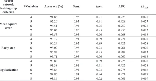
Table 4 shows the best classiication results obtained using SVM classiiers with GRBF and Polynomial kernels respectively and using the best 4, 5, 6, 7 and 8 features as input variables, varying the kernels’ orders from one to ive. All subsets shown

in Table 3 were used as input to the SVM classiiers

but, as seen in Table 5, the classiier performance does not vary signiicantly by inserting new features.

Neural networks

The performance of the three stop training criteria mentioned, mean square error, regularization and early stop with all 22 features used as input variables and different architectures, 22-5-5-1, 22-8-8-1 and 22-10-10-1 are shown in Table 5, where one can ind the accuracy, sensitivity, speciicity and AUC for each of these combinations.

Table 6 shows the accuracy, sensitivity, speciicity and AUC for the best 4, 5, 6, 7 and 8 input variables selected with scalar selection technique with correlation, with mean square error, early stop and regularization

Table 3. Best values of accuracy, sensitivity, speciicity and AUC obtained with SVM classiiers using two different kernels, GRBF and polynomial, varying their orders from one to ive and the C parameter from 0.03 to 8. All the 22 features were used as input variables.

Kernel Order C Accuracy

(%) Sens. Spec. AUC SEAUC

RBF

1 1.4 83 0.70 0.95 0.831 0.041

2 2.8 89 0.90 0.88 0.891 0.034

3 0.125 89 0.88 0.90 0.891 0.034

4 1.2 88 0.90 0.86 0.881 0.035

5 1.2 88 0.92 0.84 0.882 0.035

Mean value 87.40 0.86 0.86 0.875 0.036

Polynomial

1 0.125 90 0.92 0.88 0.900 0.032

2 0.031 84 0.90 0.78 0.839 0.040

3 1 85 0.83 0.81 0.828 0.042

4 1 80 0.81 0.78 0.762 0.048

5 1 80 0.79 0.81 0.759 0.048

Mean value 83.80 0.87 0.81 0.817 0.042

Table 4. Best accuracy, sensitivity, speciicity and AUC of the selected 4, 5, 6, 7 and 8 variables using SVM classiiers with GRBF and polynomial kernel. The pair (order, C) used is the one that achieved best results using the whole set of features.

Neural network training stop

criterion

#Variables Accuracy (%) Sens. Spec. AUC SE_AUC

Mean square error

4 91.83 0.93 0.91 0.928 0.027

5 92.20 0.93 0.91 0.928 0.027

6 94.51 0.94 0.95 0.957 0.021

7 95.03 0.95 0.95 0.953 0.022

8 95.55 0.95 0.96 0.968 0.018

Early stop

4 90.19 0.91 0.89 0.924 0.028

5 90.24 0.92 0.89 0.923 0.028

6 93.02 0.93 0.93 0.961 0.020

7 95.92 0.96 0.95 0.984 0.013

8 95.71 0.95 0.96 0.969 0.018

Regularization

4 90.88 0.92 0.89 0.926 0.028

5 91.38 0.91 0.91 0.922 0.028

6 93.86 0.94 0.93 0.975 0.016

7 94.86 0.94 0.94 0.971 0.017

training stop criteria, and 4-5-5-1, 5-5-5-1, 6-5-5-1, 7-5-5-1 and 8-5-5-1 architectures.

Table 7, adapted from the study of Flores et al. (2015), shows the performance of some previous studies published for breast cancer classiication. In this Table are shown: the category of the study - M, T or C (M – studies that use morphological characteristics, T – studies that use texture features and C – studies that use both types of features), the Mean value of Area Under ROC Curve - AUC, the standard deviation or AUC – SD and the coeficient of variation CV (SD/AUC).

Discussion

Analyzing the results shown in Table 3, when using the whole features dataset as input, the best mean accuracy value of the SVM classiier, 87.40%, was

obtained with RBF kernel. The mean AUC of RBF kernel was 0.875, while the mean AUC of Polynomial kernel was 0.817. Assessing the signiicance of the difference between the areas that lie under these two ROC curves (Hanley and McNeil, 1982), we found that P = 0.149 > 0.05, the null hypothesis should not be rejected (i.e., the SVM classiier with RBF kernel was not superior to the SVM classiier with polynomial kernel, at the 5% signiicance level).

As shown in Table 4, one can observe that concerning SVM classiiers with polynomial kernel, the scalar feature selection technique with correlation does not improve the value of AUC performance regarding the use of the 22 features. Using the RBF kernel, the same technique slightly improves the values of AUC, when using 6 and 7 characteristics, regarding the 22 features.

Table 5. Accuracy, sensitivity, speciicity and AUC of three neural network architectures, for mean square error, early stop and regularization training stop criteria. All the 22 features were used as input.

Neural network training

stop criterion Architecture Accuracy (%) Sens. Spec. AUC SEAUC

Mean square error

22-5-5-1 95.55 0.96 0.95 0.975 0.016

22-8-8-1 95.03 0.96 0.94 0.974 0.016

10-10-1 95.52 0.97 0.94 0.947 0.023

Mean value 95.37 0.96 0.94 0.965 0.018

Early stop

22-5-5-1 96.98 0.97 0.96 0.984 0.012

22-8-8-1 93.88 0.94 0.94 0.978 0.015

22-10-10-1 94.87 0.94 0.93 0.979 0.015

Mean value 95.24 0.95 0.94 0.980 0.014

Regularization

22-5-5-1 96.47 0.98 0.95 0.978 0.015

22-8-8-1 95.55 0.97 0.94 0.968 0.018

22-10-10-1 96.17 0.98 0.95 0.973 0.017

Mean value 96.06 0.97 0.94 0.973 0.017

Table 6. Accuracy, sensitivity, speciicity and AUC of a neural network with the best 4, 5, 6, 7 and 8 input variables, for mean square error, early stop and regularization training stop criteria, with 4-5-5-1, 5-5-5-1, 6-5-5-1, 7-5-5-1 and 8-5-5-1 architectures.

Neural network training

stop criterion #Variables Accuracy (%) Sens. Spec. AUC SEAUC

Mean square error

4 91.83 0.93 0.91 0.928 0.027

5 92.20 0.93 0.91 0.928 0.027

6 94.51 0.94 0.95 0.957 0.021

7 95.03 0.95 0.95 0.953 0.022

8 95.55 0.95 0.96 0.968 0.018

Early stop

4 90.19 0.91 0.89 0.924 0.028

5 90.24 0.92 0.89 0.923 0.028

6 93.02 0.93 0.93 0.961 0.020

7 95.92 0.96 0.95 0.984 0.013

8 95.71 0.95 0.96 0.969 0.018

Regularization

4 90.88 0.92 0.89 0.926 0.028

5 91.38 0.91 0.91 0.922 0.028

6 93.86 0.94 0.93 0.975 0.016

7 94.86 0.94 0.94 0.971 0.017

The best accuracy value obtained with SVM classiiers, 91%, was achieved using a RBF kernel and the best 6 features. It corresponds to an AUC of 0.911. With the whole set of features a mean AUC of 0.875 was obtained. Assessing the signiicance of the difference between the areas that lie under these two ROC curves (Hanley and McNeil, 1982), we found that P = 0.221 > 0.05, the null hypothesis should be rejected (i.e., the SVM classiier with 6 features was not superior to the classiier with whole features, at the 5% signiicance level).

Although we tested many different values of C in order to improve the classiication performance, Tables 3 shows that the best results were obtained varying C from 0.031 to 2.8.

Regarding neural networks performance in terms of AUC, Table 4 shows that, when using the 22 characteristics, regularization and early stop neural network criteria performed better than mean square error criterion. This behavior is due the fact that the irst two criteria are used to improve neural network generalization. The best mean value of AUC, 0.980, was obtained when using the architecture 22-5-5-1 and the early stop criterion.

Comparing the results in Tables 5 and 6, the following can be seen: for the mean square error, both AUC and accuracy obtained with 8 features are equal to the ones obtained with 22 features, for early stop criterion, the best performance is obtained with the best 7 selected features. The AUC value is equal to the one obtained with 22 features. The best mean value of AUC obtained with neural networks, 0.980, is superior to the best mean value obtained with the SVM classiier, 0.875. Assessing the signiicance of

the difference between the areas that lie under these two ROC curves, we found that P = 0.003 < 0.05, the null hypothesis should be rejected (i.e., the neural network classiier with early stop criterion is superior to SVM classiier, at the 5% signiicance level).

Although, in terms of AUC, there are no statistical differences in the results obtained with a lower number of features and with the whole set of features, we understand that feature selection is an important stage of the classiication process as it reduces the features vector dimensionality removing possible redundancy, iltering noises and therefore helping improving the classiiers and reducing computational efforts, as can be noticed with the SVM classiier.

Using the minimal-redundancy maximal-relevance (mrMR) criterion, based on mutual information (MI) technique, Flores et al. (2015) proposed the use of a reduced set with 5 morphological features for malignant lesion detection in BUS images, namely elliptic normalized skeleton, orientation, number protuberances and depressions, depth-to-width ratio and overlap ratio. In this study however, the best results obtained with a reduced set of 7 features: convexity, lobulation index, elliptic normalized skeleton, proportional distance, elliptic normalized circumference, depth-to-width ratio average distance and normalized residual value. Comparing these two subsets, we notice that they have a different number of features, and there is an overlap of only two variables: elliptical normalized skeleton and depth-to-width ratio. This difference suggests that the classiications results depends both on the feature selection method and on classiiers used.

Table 7. Statistical results of distinct feature sets in terms of AUC value, where SD, and CV are the standard deviation and coeficient of variation attained by each set. The sets are ordered from the best to the worst classiication performance (adapted from Flores et al., 2015).

Study Category Mean SD CV

This study (neural network with

regularization) M 0.984 0.012 0.012

Chen et al. (2003) M 0.952 0.018 0.008

Flores et al. (2015) M 0.942 0.009 0.008

Alvarenga et al. (2010) M 0.916 0.013 0.010

Horsch et al. (2002) C 0.915 0.009 0.008

Shen et al. (2007) C 0.904 0.011 0.010

Flores et al. (2015) T 0.897 0.009 0.010

Huang et al. (2008) M 0.886 0.031 0.034

Chen et al. (2005) T 0.818 0.022 0.019

Chang et al. (2003) T 0.801 0.020 0.021

Huang et al. (2006) T 0.797 0.018 0.023

Alvarenga et al. (2012) C 0.635 0.129 0.015

Yang et al. (2013) T 0.581 0.105 0.019

Alvarenga et al. (2007) T 0.565 0.036 0.018

The results presented in Table 7 show that the improvement in accuracy and AUC over time is incrementally. A direct comparison of the values is not possible, because the image databases used in these studies were extracted from different populations and the image quality is different, inducing a different behavior of the classiiers. The studies of Alvarenga et al. (2007, 2010, 2012), Flores et al.

(2015), and this study, nevertheless, used different samples of a same population and the image database has the same quality. In the sequence, we compare the best results of these studies, the one reported by study of Flores et al. (2015), with the result obtained in this study.

The best mean value of AUC obtained is this study, 0.980, is better than the value of 0.942, obtained by Flores et al. (2015) (see Table 7) using a different sample of a same population (413 benign and 228 malignant lesions). Assessing the signiicance of the difference between the areas that lie under these two ROC curves, we found that P = 0.011 < 0.05, the null hypothesis should be rejected (ie, the AUC obtained in this work is superior to the value of AUC obtained in the work of Flores et al. (2015), at the 5% signiicance level).

Acknowledgements

We would like to thanks CAPES for granting scholarships for one of the authors.

References

Alvarenga AV, Infantosi AFC, Pereira WCA, Azevedo CM. Complexity curve and grey level co-occurrence matrix in the texture evaluation of breast tumor on ultrasound images. Medical Physics. 2007; 34(2):379-87. PMid:17388154. http://dx.doi.org/10.1118/1.2401039.

Alvarenga AV, Infantosi AFC, Pereira WCA, Azevedo CM. Assessing the performance of morphological parameters in distinguishing breast tumors on ultrasound images. Medical Engineering & Physics. 2010; 32(1):49-56. PMid:19926514. http://dx.doi.org/10.1016/j.medengphy.2009.10.007. Alvarenga AV, Infantosi AFC, Pereira WCA, Azevedo CM. Assessineg the combined performance of texture and morphological parameters in distinguishing breast tumors in ultrasound images. Medical Physics. 2012; 39(12):7350-8. PMid:23231284.http://dx.doi.org/10.1118/1.4766268. Alvarenga AV, Pereira WCA, Infantosi AFC, Azevedo CM. Classification of breast tumours on ultrasound images using morphometric parameters. In: Ruano MG, Ruano AE, editors. Proceedings of the International Workshop on Intelligent Signal Processing; 2005 Sept 1-3; Algarve, Portugal. Piscataway: IEEE; 2005. p. 206-10.

Chang RF, Wu W-J, Moon WK, Chen D-R. Improvement in breast tumor discrimination by support vector machines and speckle-emphasis texture analysis. Ultrasound in Medicine

& Biology. 2003; 29(5):679-86. PMid:12754067.http:// dx.doi.org/10.1016/S0301-5629(02)00788-3.

Chen C-M, Chou Y-H, Han K-C, Hung G-S, Tiu C-M, Chiou H-J, Chiou SY. Breast lesions on sonograms: computer-aided diagnosis with nearly setting-independent features and artificial neural networks. Radiology. 2003; 226(2):504-14. PMid:12563146.http://dx.doi.org/10.1148/ radiol.2262011843.

Chen D-R, Chang R-F, Chen C-J, Ho M-F, Kuo S-J, Chen S-T, Hung S-J and Moon W-K. Classification of breast ultrasound images using fractal feature. Clinical Imaging. 2005; 29(4):235-45.

Chen D-R, Chang R-F, Huang Y-L. Computer-aided diagnosis applied to us of solid breast nodules by using neural networks. Radiology. 1999; 213(2):407-12. PMid:10551220.http:// dx.doi.org/10.1148/radiology.213.2.r99nv13407. Cheng HD, Shan J, Ju W, Guo Y, Zhang L. Automated breast cancer detection and classification using ultrasound images: a survey. Pattern Recognition. 2010; 43(1):299-317. http:// dx.doi.org/10.1016/j.patcog.2009.05.012.

Chiang HK, Tiu C-M, Hung G-S, Wu S-C, Chang TY, Chou Y-H. Stepwise logistic regression analysis of tumor contour features for breast ultrasound diagnosis. In: IEEE International Ultrasonics Symposium (IUS); 2001; Atlanta, USA. New York: IEEE; 2001. v. 2, p. 1303-6.

Dennis MA, Parker SH, Klaus AJ, Stavros AT, Kaske TI, Clark SB. Breast biopsy avoidance: The value of normal mammograms and normal sonograms in the setting of a palpable lump. Radiology. 2001; 219(1):186-91. PMid:11274555. http://dx.doi.org/10.1148/radiology.219.1.r01ap35186. Doan CD, Liong S-Y, editors. Generalization for multilayer neural network: Bayesian regularization or early stopping. In: Proceedings of the 2nd Conference of the Asia Pacific Association of Hydrology and Water Resources (APHW 2004); 2004 Jun 5-9; Singapore. Hanoi: Labor and Social Publisher; 2004. p. 5-8.

Duda RO, Hart PE, Stork DG. Pattern classification. 2nd ed. New York: Wiley-Interscience; 2000.

Flores WG, Pereira WCA, Infantosi AFC. Improving classification performance of breast lesions on ultrasonography. Pattern Recognition. 2015; 48(4):1125-36. http://dx.doi. org/10.1016/j.patcog.2014.06.006.

Flores WG. Desarrollo de una metodología computacional para la clasificación de lesiones de mama en imágenes ultrasónicas [thesis]. México: Instituto Politécnico Nacional; 2009. Hagan MT, Demuth HB, Beale MH, De Jesus O. Neural network design [internet] 2nd ed. 2016 [cited 2013 Dec 09]. Available from: http://www.mathworks.com/products/ neural-network/description6.html

Hanley JA, McNeil BJ. The meaning and use of the area under a Receiver Operating Characteristic (ROC) curve. Radiology. 1982; 143(1):29-36. PMid:7063747.http:// dx.doi.org/10.1148/radiology.143.1.7063747.

Horsch K, Giger ML, Venta LA, Vyborny CJ. Computerized diagnosis of breast lesions on ultrasound. Medical Physics. 2002; 29(2):157-64. PMid:11865987. http://dx.doi. org/10.1118/1.1429239.

Huang YL, Chen DR, Jiang YR, Kuo SJ, Wu HK, Moon WK. Computer-aided diagnosis using morphological features for classifying breast lesions on ultrasound. Ultrasound in Obstetrics & Gynecology. 2008; 32(4):565-72. PMid:18383556.http://dx.doi.org/10.1002/uog.5205. Huang YL, Wang KL, Chen D-R. Diagnosis of breast tumors with ultrasonic texture analysis using support vector machines. Neural Computing & Applications. 2006; 15(2):164-9. http://dx.doi.org/10.1007/s00521-005-0019-5. Instituto Nacional do Câncer – INCA. Ministério da Saúde. [internet]. Rio de Janeiro: INCA; 2015 [cited 2015 Oct 02] Available from: http://www2.inca.gov.br/wps/wcm/connect/ tiposdecancer/site/home/mama/deteccao_precoce Kohavi R. A study of cross-validation and bootstrap for accuracy estimation and model selection. In: Proceedings of the 14th International Joint Conference on Artificial Intelligence; 1995. Montreal, Canada. San Francisco: Morgan Kaufmann Publishers; 1995. p. 1137-43. Kramer D, Aghdasi F. Texture analysis techniques for the classification of microcalcifications in digitised mammograms. In: Proceedings of the IEEE AFRICON’99 Conference; 1999 Sept 28-Oct 1; Cape Town, South Africa. New York: IEEE; 1999. v. 1, p. 395-400.

Kuo W-J, Chang R-F, Chen D-R, Lee C. Data mining with decision trees for diagnosis of breast tumor in medical ultrasonic images. Breast Cancer Research and Treatment. 2001; 66(1):51-7. PMid:11368410.http://dx.doi. org/10.1023/A:1010676701382.

Leisch F, Jain LC, Hornik K. Cross-validation with active pattern selection for neural-network classifiers. IEEE Transactions on Neural Networks. 1998; 9(1):35-41. PMid:18252427.http://dx.doi.org/10.1109/72.655027. Moré J. The levenberg-marquardt algorithm: implementation and theory. In: Watson GA, editor. Numerical analysis. Heidelberg: Springer; 1978. p. 105-16. Lecture Notes in Mathematics, 630.

Piliouras N, Kalatzis I, Dimitropoulos N, Cavouras D. Development of the cubic least squares mapping linear-kernel support vector machine classifier for improving the characterization of breast lesions on ultrasound.

Computerized Medical Imaging and Graphics. 2004; 28(5):247-55. PMid:15249070.http://dx.doi.org/10.1016/j. compmedimag.2004.04.003.

Renjie L, Tao W, Zengchang Q. Classification of benign and malignant breast tumors in ultrasound images based on multiple sonographic and textural features. In: International Conference on Intelligent Human-Machine Systems and Cybernetics (IHMSC 2011); 2011 Aug 26-27; Hangzhou, China. Los Alamitos: IEEE Computer Society; 2011. p. 71-4. Shen WC, Chang RF, Moon WK, Chou YH, Huang CS. Breast ultrasound computer-aided diagnosis using bi-rads features. Academic Radiology. 2007; 14(8):928-39. PMid:17659238. http://dx.doi.org/10.1016/j.acra.2007.04.016.

Skaane P. Ultrasonography as adjunct to mammography in the evaluation of breast tumors. Acta Radiologica. Supplementum. 1999; 420:1-47. PMid:10693544. Sociedade Brasileira de Cancerologia. [internet]. Salvador: Sociedade Brasileira de Cancerologia; 2015 [cited 2015 Oct 02] Available from: http://www.sbcancer.org.br/home2/site/ index.php?option=com_content&view=article&id=110:ca ncer-de-mama&catid=29&Itemid=123

Theodoridis S, Koutroumbas K. Pattern recognition. 4th ed. Cambridge: Academic Press; 2008.

Uniyal N, Eskandari H, Abolmaesumi P, Sojoudi S, Gordon P, Warren L, Rohling RN, Salcudean SE, Moradi M. A new approach to ultrasonic detection of malignant breast tumors. In: IEEE International Ultrasonics Symposium (IUS); 2013 July; Prague, Czech Republic. New York: IEEE; 2013. p. 96-9.

World Health Organization – WHO. Breast cancer: prevention and control [internet]. Geneva: WHO; 2014 [cited 2015 Oct 02] Available from: http://www.who.int/cancer/detection/ breastcancer/en/

Wu W-J, Moon WK. Ultrasound breast tumor image computer-aided diagnosis with texture and morphological features. Academic Radiology. 2008; 15(7):873-80. PMid:18572123. http://dx.doi.org/10.1016/j.acra.2008.01.010.

Yang MC, Moon WK, Wang YCF, Bae MS, Huang CS, Chen JH, Chang RF. Robust texture analysis using multi-resolution gray-scale invariant features for breast sonographic tumor diagnosis. IEEE Transactions on Medical Imaging. 2013; 32(12):2262-73. PMid:24001985.http://dx.doi.org/10.1109/ TMI.2013.2279938.

Authors

Carmina Dessana Lima Nascimento1, Sérgio Deodoro de Souza Silva1, Thales Araújo da Silva1, Wagner Coelho de

Albuquerque Pereira2, Marly Guimarães Fernandes Costa1, Cicero Ferreira Fernandes Costa Filho1_*

1 Centro de Tecnologia Eletrônica e da Informação, Universidade Federal do Amazonas – UFAM, Avenida General

Rodrigo Otávio Jordão Ramos, 3000, Aleixo, Campus Universitário - Setor Norte, Pavilhão Ceteli, CEP 69077-000, Manaus, AM, Brazil.

2 Programa de Engenharia Biomédica, Instituto Alberto Luiz Coimbra de Pós-Graduação e Pesquisa em Engenharia –