Measurement of turbulence in the oceanic mixed layer using Synthetic Aperture Radar (SAR)

(1)

OSD

9, 2851–2883, 2012

Measurement of turbulence using

SAR

S. G. George and A. R. L. Tatnall

Title Page

Abstract Introduction

Conclusions References

Tables Figures

◭ ◮

Back Close

Full Screen / Esc

Printer-friendly Version Interactive Discussion

Discussion

P

a

per

|

Dis

cussion

P

a

per

|

Discussion

P

a

per

|

Discussio

n

P

a

per

|

Ocean Sci. Discuss., 9, 2851–2883, 2012 www.ocean-sci-discuss.net/9/2851/2012/ doi:10.5194/osd-9-2851-2012

Ocean Science Discussions

This discussion paper is/has been under review for the journal Ocean Science (OS). Please refer to the corresponding final paper in OS if available.

Measurement of turbulence in the oceanic

mixed layer using Synthetic Aperture

Radar (SAR)

S. G. George and A. R. L. Tatnall

Astronautics Research Group, Faculty of Engineering & the Environment, University of Southampton, Southampton, UK

Received: 25 June 2012 – Accepted: 26 August 2012 – Published: 13 September 2012 Correspondence to: S. G. George (sgg303@soton.ac.uk)

(2)

OSD

9, 2851–2883, 2012

SAR

Title Page

Tables Figures

◭ ◮

Back Close

Full Screen / Esc

Discussion

P

a

per

|

Dis

cussion

P

a

per

|

Discussion

P

a

per

|

Discussio

n

P

a

per

|

Abstract

Turbulence in the surface layer of the ocean contributes to the transfer of heat, gas and momentum across the air-sea boundary. As such, study of turbulence in the ocean sur-face layer is becoming increasingly important for understanding its effects on climate change. Direct Numerical Simulation (DNS) techniques were implemented to examine

5

the interaction of small-scale wake turbulence in the upper ocean layer with incident electromagnetic radar waves. Hydrodynamic-electromagnetic wave interaction models were invoked to demonstrate the ability of Synthetic Aperture Radar (SAR) to observe and characterise surface turbulent wake flows. A range of simulated radar images are presented for a turbulent surface current field behind a moving surface vessel, and

10

compared with the surface flow fields to investigate the impact of turbulent currents on simulated radar backscatter. This has yielded insights into the feasibility of resolv-ing small-scale turbulence with remote-sensresolv-ing radar and highlights the potential for extracting details of the flow structure and characteristics of turbulence using SAR.

1 Introduction 15

The boundary between the air and the sea plays a crucial role in regulating the thermal and gaseous balance between ocean and atmosphere. Turbulence and mixing in the near-surface layer of the ocean have considerable impact on the transfer of properties such as heat and momentum across this boundary. There is currently increasing inter-est in the e_ffect of the upper ocean layer on climate change studies, particularly in the

20

role of ocean turbulence in the exchange of carbon dioxide between air and sea: it is estimated that 25–50 % of anthropogenic CO2delivered into the air across the globe is

absorbed by the sea (Sabine et al., 2004; Khatiwala et al., 2009) and that upper ocean turbulence may play a key role in this exchange (Soloviev et al., 2007). The rates of exchange of such properties are governed by the characteristics and dynamics of the

25

(3)

OSD

9, 2851–2883, 2012

SAR

Title Page

Tables Figures

◭ ◮

Back Close

Full Screen / Esc

Discussion

P

a

per

|

Dis

cussion

P

a

per

|

Discussion

P

a

per

|

Discussio

n

P

a

per

|

Such conditions are dependent on the surface wave system and fluid mixing, and there-fore near-surface turbulence is therethere-fore a critical element in the exchange processes of gas, heat and momentum between the ocean and atmosphere (McKenna, 2000; McKenna and McGillis, 2004; Soloviev et al., 2007; Zappa et al., 2009; Veron et al., 2011). Identifying methods by which turbulent phenomena can be observed and levels

5

of small-scale turbulence in the oceanic mixed layer may be identified through remote-sensing techniques could be of benefit in quantifying the impact of the ocean mixed layer on climate change, and improving understanding of this complex system.

Turbulence is present in the ocean over a broad spectrum of spatial scales, from mesoscale and geostrophic eddies formed by global currents to small-scale turbulence

10

generated by breaking surface- or internal waves. Synthetic Aperture Radar (SAR) has shown considerable ability to remotely observe a wide range of such phenomena as shown by, for example, Chubb et al. (1999), Ivanov and Ginzburg (2002), Alpers et al. (2004) and Johannessen et al. (2005). Turbulent processes in the upper ocean layer predominantly affect SAR signatures in two ways: firstly, the primary flow

struc-15

ture and currents propagating to the surface produce wave-current interactions which cause straining of the surface distribution of short wind waves. Hence, features such as internal waves can be resolved due to their surface currents modifying the distri-bution of Bragg waves (Thompson, 1985), as well as other oceanic phenomena. Sec-ondly, fine-scale turbulence, velocity fluctuations and viscosity near the surface layer

20

act to redistribute surface wave energy at scales on the order of the radar wavelength, through the processes of viscous dissipation and downward convection of wave energy (Kitaigorodskii and Lumley, 1983; Kitaigorodskii et al., 1983; Reed et al., 1990; ¨Olmez and Milgram, 1992; True et al., 1993). Turbulence and mixing at, and near, the sea surface is therefore typically observed as a region of reduced radar backscatter, with

25

(4)

OSD

9, 2851–2883, 2012

SAR

Title Page

Tables Figures

◭ ◮

Back Close

Full Screen / Esc

Discussion

P

a

per

|

Dis

cussion

P

a

per

|

Discussion

P

a

per

|

Discussio

n

P

a

per

|

dampening of short waves. The result is reduced backscattering and increased levels of specular reflection in regions of turbulence, leading to dark patches in Normalised Radar Cross-Section (NRCS) and SAR imagery. Interaction of the surface flow with the incident wind and wave systems also produces short-wave interaction, creating a complex pattern of bright and dark regions of NRCS. The importance of near-surface

5

fluid motions on air-sea exchange processes and the ability of such motions to mod-ify the response of remote-sensing radar lead to encouraging potential for improving understanding of the oceanic mixed layer from remote measurements.

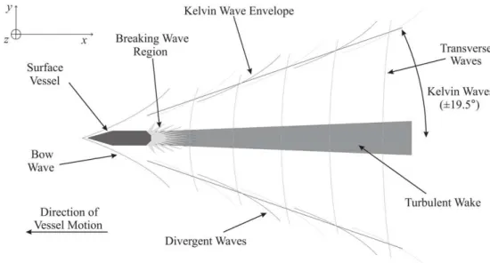
Moving surface vessels such as ships typically produce wakes which are highly vis-ible in ocean SAR images, where the region behind the vessel displays a region of

10

wake turbulence and surface currents which produce a visible backscattering response. A schematic of a typical ship wake is presented in Fig. 1, and examples of turbulent wake features in operational SAR images can be found extensively in the literature (Munk et al., 1987; Lyden et al., 1988; Milgram et al., 1993; Hennings et al., 1999; Toporkov et al., 2011). Simulation of ship-wake turbulence and the NRCS response

15

has previously been studied by, for example, Reed et al. (1990), True et al. (1993) and Fujimura et al. (2011). There has, however, been limited investigation on the impact of turbulence on short surface waves. A further challenge is that the presence of surfac-tants and oil films floating on the sea surface can often disguise the effect of turbulence due to their greater dampening impact on radar-scattering waves. The development

20

of high-resolution SARs such as TerraSAR-X has reinvigorated the interest in identify-ing small-scale ocean processes from remote observations, leadidentify-ing to recent studies of turbulent ship wakes such as Soloviev et al. (2010), Fujimura et al. (2011) and Toporkov et al. (2011). These investigations indicate that with improvement in signal-to-noise capability and spatial resolution of future SAR instrumentation, increased

discrimina-25

(5)

OSD

9, 2851–2883, 2012

SAR

Title Page

Tables Figures

◭ ◮

Back Close

Full Screen / Esc

Discussion

P

a

per

|

Dis

cussion

P

a

per

|

Discussion

P

a

per

|

Discussio

n

P

a

per

|

2 Simulation of wake turbulence and remote-sensing signatures

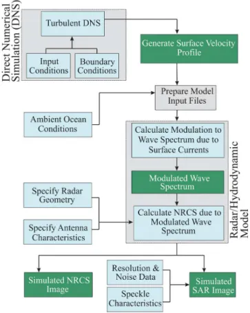
In order to examine the effect of upper ocean turbulence on radar images, a simulation procedure was constructed using a case study of a simple moving surface vessel acting as an initiator for turbulence near the fluid surface. The region aft of such a body dis-plays a rearward wake containing regions of intense turbulence and vortical flow, and

5

Direct Numerical Simulation (DNS) techniques were integrated with an ocean radar imaging model to numerically simulate turbulence near a fluid surface and derive the-oretical remote-sensing signatures. The process of translating results from turbulent simulation by DNS to simulated surface signatures in NRCS arising from the turbulent flow is presented in Fig. 2.

10

The DNS process was performed using a C/C++ numerical code solving the in-compressible Navier-Stokes equations for fluid velocity, u_i, given in Cartesian tensor notation by

∂u_i ∂t +uj

∂u_i ∂x_j =−

1

ρ ∂p ∂x_i +ν

∂2u_i

∂x_j∂x_j +Fi (1)

where i ₌ (1, 2, 3), ρ is the fluid density, ν is the kinematic viscosity, t represents

15

time,F_i represent external forcing terms,p is the fluid pressure andu_i₌(u, v, w) rep-resents velocity in the coordinate system x_i₌(x, y, z). Simulations were performed using the IRIDIS3 high-performance computing facility at the University of Southamp-ton. The algorithm solves with su_fficient numerical accuracy to represent all turbulence scales (Thomas and Williams, 1997; Archer, 2008). Modelling of a representative

sur-20

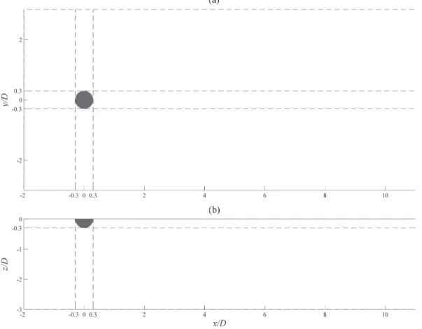
face body was applied through body-force parameterisation using an immersed bound-ary method, and a non-dimensional freestream velocity, U, applied in the x-direction to mimic the body moving in a fixed reference frame. The vessel was characterised by a submerged half-sphere, where F_i are the external body forces due to the vir-tual body surface B ₌ (B_x,B_y,B_z). The submerged half-sphere was modelled using

25

(6)

OSD

9, 2851–2883, 2012

SAR

Title Page

Tables Figures

◭ ◮

Back Close

Full Screen / Esc

Discussion

P

a

per

|

Dis

cussion

P

a

per

|

Discussion

P

a

per

|

Discussio

n

P

a

per

|

representation of a towed surface vessel. The no-slip boundary condition was applied to the embedded surface. A schematic of the DNS domain and parameterisation of the body is shown in Fig. 3. No efforts to replicate the profile of any existing surface vessel were made, and the simulation also neglects other features of the wake presented in Fig. 1, such as the Kelvin and transverse wave systems and the occurrence of

break-5

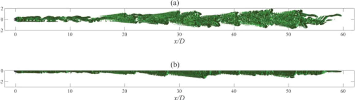
ing waves. The wake is hence simulated as a region of drag behind the body which causes the flow to decelerate and generate a region of mixing and vorticity, and a tur-bulent wake analogous to that of a surface moving vessel. A representative output from the DNS process is shown in Fig. 4, showing an isosurface of the second invariant of the velocity gradient tensor (Π), which is a useful visual marker for turbulent structure

10

and vorticity.

The three-dimensional domain was formed of approximately 70 million grid points: 2112 in thex-direction (direction of vessel motion), 256 in they-direction (perpendic-ular to vessel motion in surface plane), and 128 in thez-direction (vertical direction); a schematic of this domain is presented in Fig. 3. A fixed boundary (under the

rigid-15

lid approximation) was applied to the upper surface and periodic boundary conditions applied to the edges of the domain. The numerical flow was processed until the on-set of fully-developed turbulence; at desired time steps, pausing the simulation to write to disk the velocity (u_i) and pressure (p) data at each grid point in the domain. The three-dimensional velocity data was then retrieved, returned to dimensional form and

20

exported to the radar image model to simulate modulation of the surface wave spec-trum due to turbulent currents, and subsequently to derive simulated NRCS imagery. The reference frame was adjusted to remain fixed with respect to the fluid, creating a turbulent wake equivalent to a simulated vessel moving over a stationary water sur-face.

25

(7)

OSD

9, 2851–2883, 2012

SAR

Title Page

Tables Figures

◭ ◮

Back Close

Full Screen / Esc

Discussion

P

a

per

|

Dis

cussion

P

a

per

|

Discussion

P

a

per

|

Discussio

n

P

a

per

|

spectrum. The radar ocean imaging model employed in the study was the M4S Toolkit v3.2.0 (hereby referred to as “M4S”). A complete theory of the model may be found in Romeiser et al. (1997) and Romeiser and Alpers (1997); its operation is summarised here. Since it is a quantity conserved by an ocean wave system in the presence of the surface currents, wave action spectral density is commonly computed in wave-current

5

interaction models to examine the distribution of surface backscattering waves (Phillips, 1966). The M4Sw320 algorithm of M4S approximates modulation of the wave spectrum due to the surface wake profile and specification of a characteristic wind field present at reference height 10 m above the simulated ocean surface. In all cases, a uniform wind field was applied to the domain with varying magnitude and direction applied in

10

di_fferent tests. The wave spectral data is then exchanged with the radar simulation module M4Sr320 of M4S to approximate the radar backscattering response based on the modulated surface, specified radar instrument parameters and the desired obser-vation geometry. Specification of the radar operating frequency f₀ (GHz), incidence angle θ₀ (degrees), instrument polarisation (HH/HV/VH/VV), and look direction with

15

respect to thex-axis (defined in degrees) are required in the M4S batch file to com-pute the NRCS backscatter response. The algorithm is described by the Two-Scale Model formulation of Wright (1968), upon which the Bragg NRCS contribution to radar backscatter,σ_0,Bragg, is proportional to the wave height spectral densityψ(k) of waves travelling toward/away from the radar look direction at wavenumberkB, given by

20

kB=2k0sinθ0 (2)

k0=2πf_c0 (3)

where k0 denotes the radar wavenumber vector and c is the speed of light. Addi-tional contribution to the NRCS is provided by the orientation of the backscattering

25

(8)

OSD

9, 2851–2883, 2012

SAR

Title Page

Tables Figures

◭ ◮

Back Close

Full Screen / Esc

Discussion

P

a

per

|

Dis

cussion

P

a

per

|

Discussion

P

a

per

|

Discussio

n

P

a

per

|

backscattering response of Bragg waves only is referred to here as the Bragg NRCS

σ_0,Bragg, whereas the two-scale response is the composite spectrum NRCS,σ₀.

Comments

There remain some comments regarding the consistency of the modelling and simula-tion techniques used in this research and the characteristics of small-scale turbulence,

5

which are raised here.

Turbulence of a fluid, particularly at small scales near the ocean surface, implies a rapid fluctuation of quantities over small spatial distances. Turbulence is thus by a highly-energetic state of mixing, and one which may be characterised by changes of high gradients of velocity at small scales. Typical radar ocean imaging algorithms

10

use the theory of weak hydrodynamic interactions in order to process modulated wave spectra using the conservation of wave action spectral density (LeBlond and Mysak, 1978). This theory, within the framework of Geometrical Optics under the WKB approx-imation assumes that disturbances in surface current are small when compared to the primary ocean wavelengths, and that the current field can be assumed to stationary

15

as waves propagate through it. Hence, these assumptions are an oversimplification in cases where there are very strong gradients in the surface current, and therefore there may be substantial modulation of some waves that nonlinearities occur that are not represented correctly in the specified wave energy balance. Time scales of current variation must not be so rapid that many wave components feel current changes and

20

acceleration as they navigate the current field: in this turbulent case, there may be, lo-cally, rapid fluctuation of velocity at small scales even though the mean surface current (at the longer length scales) may be assumed to be slowly-varying in time in compar-ison with the wave’s journey across the domain. The mean current may therefore be considered stationary or “frozen” as wave propagation is calculated, and application of

25

hydrodynamic wave interaction techniques may be justified.

(9)

OSD

9, 2851–2883, 2012

SAR

Title Page

Tables Figures

◭ ◮

Back Close

Full Screen / Esc

Discussion

P

a

per

|

Dis

cussion

P

a

per

|

Discussion

P

a

per

|

Discussio

n

P

a

per

|

presence of a moving surface vessel. The interaction of turbulence and waves may be considered weak if the energy gained by the turbulence through interaction with waves is small when compared with the energy transfer due to internal turbulence interactions. Hence, the accuracy of the simulation may be improved by including in the wave action conservation calculation the e_ffects of exchange of energy between the turbulence and

5

the wave system: some authors have operated models which directly represent turbu-lent energy dissipation (spectral modification caused by turbuturbu-lent fluctuations within the wake), such as Milgram et al. (1993) and True et al. (1993). In the discussion presented in this paper, the effects of turbulent dissipation of short-wave energy have not been accounted for in the calculation of the modulated wave spectrum. Results presented

10

by ¨Olmez and Milgram (1992) indicate that energy dissipation due to turbulent fluc-tuations may be significant for regions of intense small-scale mixing (particularly ship wakes), and thus examination of the effect of dissipation of wave energy by subsurface turbulence on SAR remote-sensing signatures should be applied in future numerical work.

15

Simulation of turbulent ship wakes has been studied extensively in the literature by a range of authors using radar/hydrodynamic interaction theory (Lyden et al., 1985; True et al., 1993; Reed and Milgram, 2002). There is limited discussion of the im-pact of the turbulent wake flow on the applicability of the governing equations oper-ated by radar ocean imaging models, however many researchers have successfully

20

applied such methods to wake turbulence, including turbulence at small scales in the far wake of a ship (Fujimura et al., 2011). Since the large-scale turbulent motions may be considered as “slowly-varying” when compared to the surface wave field, and the small-scale turbulent motions (when averaged) do not affect the larger picture, it may be assumed that the wave action computation provides a reasonable approximation

25

(10)

OSD

9, 2851–2883, 2012

SAR

Title Page

Tables Figures

◭ ◮

Back Close

Full Screen / Esc

Discussion

P

a

per

|

Dis

cussion

P

a

per

|

Discussion

P

a

per

|

Discussio

n

P

a

per

|

3 Results and discussion

The full simulation strategy integrating DNS and hydrodynamic/electromagnetic wave modelling to simulate backscatter responses of surface wake turbulence was per-formed to examine radar signatures under a range of conditions. A selection of the obtained results are presented here. A key focus of the study was to examine the

fea-5

sibility for extracting information on the structure of near-surface fluid turbulence using remote-sensing instrumentation. Therefore, experiments primarily focussed on the vis-ibility of such structure from simulated Bragg NRCS and composite spectrum NRCS backscatter imagery.

3.1 Observation of turbulent surface structure 10

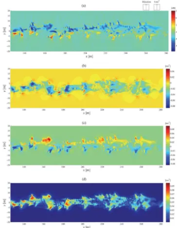
A representative plot of a region of the wake commencing approximately 130 m aft of the vessel, rendered in 5.3 GHz (C-band) composite spectrum NRCS at 23◦_incidence

and HH-polarisation, is presented in Fig. 5a. The surface u- and v-velocity profiles for this region of the wake are shown in Fig. 5b, c, respectively. The wake profile is formed of a domain 1000 grid points long in the x-direction, and 250 points in the

15

y-direction. Peak currents in the turbulent region are observed to be in the region of 0–0.1 m s−1_{in magnitude, as shown by Fig. 5d. Qualitative comparisons may be drawn}

between the surface velocity profiles and the modulated NRCS response; in particular, the influence of velocity gradients and fluctuations on the observed NRCS distribution, and how details of the flow structure present in the surface velocity profiles can be

20

resolved by the simulated radar. The NRCS modulation responds to current patterns within the wake arising from fluctuations of the turbulent flow (due to wave-current interaction), hence permitting the surface flow structure of the wake to be observed and identified. Such structure is illustrated by the distribution of flow currents and hence the network of eddies which define the turbulent flow. The content and character of the

25

(11)

OSD

9, 2851–2883, 2012

SAR

Title Page

Tables Figures

◭ ◮

Back Close

Full Screen / Esc

Discussion

P

a

per

|

Dis

cussion

P

a

per

|

Discussion

P

a

per

|

Discussio

n

P

a

per

|

Fujimura et al. (2011), showing similar instances of the velocity structure of turbulence propagating through the simulated radar imaging process into modulated NRCS.

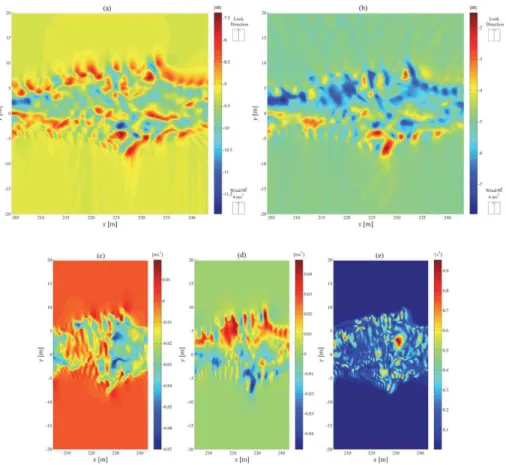
A portion of the wake approximately 205–245 m aft of the surface vessel for a simu-lated 5.3 GHz (C-band) radar is depicted in Fig. 6, where 6a displays the Bragg NRCS response, 6b the composite spectrum NRCS response, and 6c, d, e represent the

sur-5

faceu-velocity,v-velocity and vorticity, respectively. Details of the flow structure present in the velocity data can be resolved in the NRCS responses, particularly the relation-ship between the composite spectrum NRCS and the spanwisev-velocity highlighting interaction with wind in they-direction: this can be observed on the upper and lower edges of the wake where there is interaction between the wake velocity, the ambient

10

wind and the quiescent fluid outside the wake. It is also encouraging that characteris-tics of the internal flow structure, i.e. the velocity fluctuations along the centre line of the wake axis, produce modulation of the surface wave spectrum and are resolved in the NRCS response. Kelvin-Helmholtz billows arising from shear instability within the wake flow can also be observed in the DNS velocity and vorticity data, visible as unstable

15

fluctuations in the surface flow characteristics at the edges of the wake region in Figs. 6c–e. These effects propagate through the integrated hydrodynamic-electromagnetic modelling process, and can be observed in the in simulated Bragg and composite spectrum NRCS images, such as in Figs. 6a–b.

The results obtained here indicate that, where present, characteristics of the

small-20

scale turbulent flow structure in a surface wake propagates through the process of cal-culating wave-current interaction, and are thus rendered visible in NRCS. This demon-strates that the wake flow has measurable influence the NRCS response, and this may be developed further to understand more about the relationship between near-surface turbulence and radar backscatter.

25

3.2 Instrument frequency

(12)

OSD

9, 2851–2883, 2012

SAR

Title Page

Tables Figures

◭ ◮

Back Close

Full Screen / Esc

Discussion

P

a

per

|

Dis

cussion

P

a

per

|

Discussion

P

a

per

|

Discussio

n

P

a

per

|

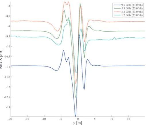
on wave height spectral density is not constant across the spectrum, the backscatter-ing response may display significant variation of NRCS withkB. Changes in kB are applied here by altering the operating frequency according to Eqs. (2)–(3), while keep-ing fixed the incidence angle of the instrument. Perturbkeep-ing the operatkeep-ing frequency of the simulated instrument used to generate the NRCS response therefore has the

5

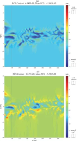
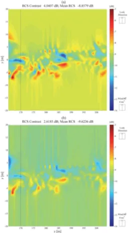
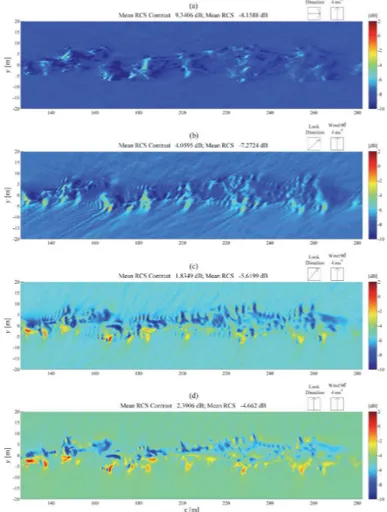
ability to alter the distribution of the Bragg-scale waves primarily responsible for radar backscatter and hence the composition of turbulent flow structure that is translated to NRCS. Figures 7, 8 depict a portion of the wake approximately 165–205 m aft of the surface vessel rendered in Bragg NRCS at X-, C-, S- and L-band plotted on the same colour axis. These simulations assume constant parameters for HH-polarisation, 23◦

10

angle of incidence and a look direction in the positivey-direction. A line is drawn at a position approximately 170 m to depict the location of transects taken of the Bragg NRCS across the wake: varying the operating frequency reveals differing effects of the flow structure at different regions of the surface wave spectrum, highlighting different areas of primary modulation. Presented in Fig. 9 is a composite plot of transects of

15

Bragg NRCS at the frequencies applied in Figs. 7, 8. These results prove that modu-lation of the surface wave spectrum is dependent on the operating radar wavenumber and that the visibility of small-scale features on the surface may vary considerably with operating frequency. There is also variation in the resolved modulation depth (variation between maximum and minimum NRCS values), and mean NRCS (average across the

20

image) value, both of which may influence the desired operating frequency to maximise the ability to resolve small-scale turbulent features. While the S-band plot of Fig. 8a displays the largest average NRCS across the image (which may be important in pres-ence of signal-to-noise losses), the C-band simulation displayed in Fig. 7b displays the largest range of NRCS across the applied transect, allowing the potential to extract

25

(13)

OSD

9, 2851–2883, 2012

SAR

Title Page

Tables Figures

◭ ◮

Back Close

Full Screen / Esc

Discussion

P

a

per

|

Dis

cussion

P

a

per

|

Discussion

P

a

per

|

Discussio

n

P

a

per

|

3.3 Viewing orientation

Since the backscattering response primarily captures Bragg-scale waves travelling to-ward/away from the instrument look direction, there is an associated directionality of the modulated wave spectrum which can be observed by rotating the instrument orien-tation with respect to both the centre axis of the wake and the direction of the applied

5

wind field. This has the potential to reveal further information about the character of the turbulent flow from NRCS images viewed from varying perspectives; observed in Fig. 10, where the impact of varying the instrument look direction from 10a 0◦_(aligned

with thex-direction) to 10d 90◦ _{(aligned with the}_x_{-direction) on the resolved structure}

of the wake is displayed. The wind is aligned in they-direction, therefore the distribution

10

of short waves is predominantly aligned in the spanwise direction; hence the primary wave-current interaction occurs along this axis where Bragg-scattering waves interact with the spanwise flow.

For a simulated image with look direction perpendicular to the applied wind, as in Fig. 10a, the structure and flow features as less easily resolved through their contrast

15

with the background NRCS: such details are more visible when the radar look is aligned in a direction with sufficient presence of short waves, e.g. Figure 10d. In the real ocean, the directionality of short wind waves is likely to be much broader than in this simple case of a uniform wind direction due to spatial variation of both wind speed and direc-tion. Therefore, these results present a “worst-case” state of conditions pertaining to

20

the variation of wake visibility with the instrument look aspect, however it is clear that maximum resolution of the turbulent currents is attainable in cases where strongest interaction with the background wave spectrum occurs.

3.4 Effect of wind speed

The simulation results obtained thus far represent an idealised case of a turbulent

25

(14)

OSD

9, 2851–2883, 2012

SAR

Title Page

Tables Figures

◭ ◮

Back Close

Full Screen / Esc

Discussion

P

a

per

|

Dis

cussion

P

a

per

|

Discussion

P

a

per

|

Discussio

n

P

a

per

|

field) has been propagated to consider the effects of wave-current interaction on radar backscatter. The dynamics of such a flow in the real ocean will be superposed onto, and interact with, multiple other fluid motions including large-scale currents, orbital wave motions and wave-breaking processes. Furthermore, the ability for SAR to resolve sur-face features is strongly dependent on the ambient spectrum of backscattering waves

5

(both capillary waves in the Bragg scattering regime and gravity waves causing surface tilting) driven by the characteristics of wind forcing. In the simulations pursued here, the characteristics of the wave spectrum propagated over the simulated wake velocity pro-file are applied by definition of a simple wind field which is uniform across the domain. In reality, there is likely to be significant spatial variation in wind speed and direction,

10

leading to spatial variation of the waves responsible for backscatter and a departure from the idealised wave-current interaction statistics computed here.

The dependence of wind speed on NRCS is illustrated by the series of plots depicted in Fig. 11, for a region of the turbulent wake beginning approximately 205 m aft of the location of the simulated surface body and for a uniform wind field aligned in the y

-15

direction. Below wind speeds of 2 m s−1_{, the mean NRCS over the image is typically}

very low since the weak forcing from the wind typically generates only a meagre dis-tribution of Bragg-scattering waves over the surface. Under such conditions, the low radar response is unlikely to permit the signature to be resolved in a true SAR image. Increasing the simulated wind speed through to medium-level winds (2 to 10 m s−1₎

dis-20

plays a rise in mean image NRCS to levels greater than−12 dB, and also an increase in

mean image contrast (taken as the average contrast across all range lines). At 2 m s−1_,

there is a mean contrast of approximately 3 dB, while levels this falls below 1 dB in wind speeds stronger than 8 m s−1_{, which may lead to insu}

fficient contrast to resolve the signature against the background. A comparison of relative contrast with

back-25

ground NRCS levels (taken in the quiescent fluid outside the wake) at different wind speeds is presented in Fig. 12b for a region of the wake approximately 85–125 m aft of the body. A representative Bragg NRCS image for wind speed of 4 m s−1 _{is presented}

(15)

OSD

9, 2851–2883, 2012

SAR

Title Page

Tables Figures

◭ ◮

Back Close

Full Screen / Esc

Discussion

P

a

per

|

Dis

cussion

P

a

per

|

Discussion

P

a

per

|

Discussio

n

P

a

per

|

Bragg NRCS in Fig. 12b demonstrate significant variation in the resolved signature with wind speed, particularly under strong winds. These results are consistent with results from a similar sensitivity study published by True et al. (1993), where increasing wind speed leads to a reduction in NRCS perturbation from background levels; although the levels of NRCS perturbation obtained by True et al. (1993) differ in magnitude from

5

those presented due to differences in the numerical model and the radar frequency used in the simulation. Overall, there is indication that the visible radar signature por-trayed by the wake turbulence can deteriorate significantly in rough ocean conditions, but that under more modest wind and sea states, the turbulent wake structure may be more easily resolved.

10

4 Conclusions

The results presented here indicate that flow structure embedded in turbulent surface wakes can be translated to and resolved by changes in radar backscatter; in particular, the ability for the currents (and current gradients) associated with small-scale wake turbulence to propagate through the integrated electromagnetic-hydrodynamic wave

15

interaction process into simulated NRCS images. The simulated radar images of small-scale upper-ocean turbulence presented in this paper are consistent with existing SAR observations of turbulent surface wakes that display a reduction of NRCS inside the turbulent wake region due to turbulent surface currents.

Numerical experiments of a simulated radar instrument were performed for a range of

20

ambient conditions and for a number of instrument configurations. These have shown that, where there is observable and interesting flow structure present in the wake, this structure can be translated through the modelling process into modulated NRCS imagery. There is encouraging potential for successful observation of such turbulent phenomena with future developments in SAR instrumentation. The surface profiles of

25

(16)

OSD

9, 2851–2883, 2012

SAR

Title Page

Tables Figures

◭ ◮

Back Close

Full Screen / Esc

Discussion

P

a

per

|

Dis

cussion

P

a

per

|

Discussion

P

a

per

|

Discussio

n

P

a

per

|

models, were found to be consistent with similar data recently presented by Fujimura et al. (2011) and with SAR ship wakes published in the literature. Currently there are limited SAR observations of small-scale turbulence primarily due to the limita-tions of spatial resolution from typical spaceborne instruments: the grid resolution of the modulated NRCS profiles shown here are around 15 cm, while typical SARs such

5

as TerraSAR-X and Envisat ASAR can achieve typical resolutions of 3 m×3 m and

12.5 m×12.5 m. When averaged to similar resolutions, the turbulence NRCS

signa-tures may deteriorate significantly and reduce the capability to observe small-scale structure. Motion of the surface and platform during generation of a real SAR image may also introduce further issues which degrade the ability. However, despite the

cur-10

rent results being preliminary, there is su_fficient indication of the feasibility of measuring turbulence with SAR in the context of future developments of spatial resolution, sensi-tivity and noise reduction. The techniques developed here provide a tool for optimizing measurement techniques and parameters, indicating the necessary requirements to observe small-scale turbulence in the upper ocean. They also provide a better

un-15

derstanding of the relationship between turbulence and radar cross-section that could enable turbulence and sources to be characterised.

These efforts have shown the ability of ocean radar image modelling to convert tur-bulent wake results from a primitive DNS model into encouraging results that resolve components of the flow structure in simulated Bragg NRCS and SAR imagery. This

20

shows promise for using SAR to investigate and observe near-surface turbulence, and may aid in revealing methods by which improvements in observation of the flow struc-ture of turbulent wake flows can be accomplished. However, further work is required to develop these relationships, and to understand the impact of surface-layer turbu-lence on radar backscattering through imaging models under a range of ambient and

25

observation conditions, turbulent processes and operational constraints.

(17)

OSD

9, 2851–2883, 2012

SAR

Title Page

Tables Figures

◭ ◮

Back Close

Full Screen / Esc

Discussion

P

a

per

|

Dis

cussion

P

a

per

|

Discussion

P

a

per

|

Discussio

n

P

a

per

|

exchanges through remote-sensing measurements. Further study may identify the po-tential to extract characteristics of turbulence dissipation or vorticity from simulated remote measurements and apply relations between such values and empirical gas exchange relationships, such as that between gas transfer rate and dissipation of Tur-bulence Kinetic Energy (TKE) discussed by Zappa et al. (2007). Alternatively, there

5

may be possibilities for estimating energy and momentum fluxes from the structure of flow in the upper ocean which may be observed using SAR: turbulent flows at the sur-face could help quantify the e_ffect of surface renewal processes which are important in estimating air-sea exchanges, as discussed by, e.g. Komori and Ueda (1982) and Banerjee and MacIntyre (2004). Comparisons may be drawn between the simulation

10

process constructed in this study, and similar numerical simulations of turbulence at the ocean-atmosphere interface using DNS and LES (Large Eddy Simulation) and relation-ships with gas exchange, for example Banerjee and MacIntyre (2004) and Shen and Yue (2006). Improving observation of subsurface processes in the oceanic mixed layer on a global scale will increase our understanding of the uptake of heat and CO2by the 15

ocean, and improve parameterisation of the fluxes associated with air-sea exchange.

Acknowledgements. The authors would like to thank Watchapon Rojanaratanangkule, Gary Coleman and Glyn Thomas at the University of Southampton for their assistance and exper-tise in running the DNS code and supplying the ship wake data. Further thanks go to Roland Romeiser of the University of Miami for use of the radar imaging model used in this study

20

and stimulating discussion regarding results. The authors acknowledge the use of the IRIDIS High Performance Computing Facility at the University of Southampton in the completion of this research. This work was performed as part of an ongoing Ph.D. project titled “Satellite Mea-surement of Ocean Turbulence” funded by the University of Southampton and the Engineering and Physical Sciences Research Council.

(18)

OSD

9, 2851–2883, 2012

SAR

Title Page

Tables Figures

◭ ◮

Back Close

Full Screen / Esc

Discussion

P

a

per

|

Dis

cussion

P

a

per

|

Discussion

P

a

per

|

Discussio

n

P

a

per

|

References

Alpers, W. R., Campbell, G., Wensink, H., and Zhang, Q.: Underwater topography, in: SAR Marine User’s Manual, edited by: Jackson, C. R. and Apel, J. R., National Oceanic and Atmospheric Administration, Washington DC, USA, 245–262, 2004, available at: http://www. sarusersmanual.com/, last access: 15 May 2012.

5

Archer, P. J.: A Numerical Study of Laminar to Turbulent Evolution and Free-Surface Interaction of a Vortex Ring, Ph. D. thesis, University of Southampton, Southampton, UK, 2008.

Banerjee, S. and MacIntyre, S.: The air-water interface: Turbulence and scalar exchange, in: Ad-vances in Coastal and Ocean Engineering vol. 9: PIV and Water Waves, edited by: Grue, J., Liu, P. L. F. and Pedersen, G. K., World Scientific, Singapore, 181–237, 2004.

10

Chubb, S. R., Askari, F., Donato, T. F., Romeiser, R., Ufermann, S., Cooper, A. L., Alpers, W. R., and Mango, S. A.: Study of Gulf Stream features with a multifrequency polarimetric SAR from the Space Shuttle, IEEE Trans. Gisci. Remote Sens., 37, 2495–2507, 1999.

Fujimura, A., Matt, S., Soloviev, A., Maingot, C., and Rhee, S. H.: The Impact of Thermal Strat-ification and Wind Stress on Sea Surface Features in SAR Imagery, IGARSS2011 IEEE

15

Geoscience and Remote Sensing Symposium, Vancouver BC, Canada, 24–29 July 2011, 2037–2040, 2011.

Hennings, I., Romeiser, R., Alpers, W. R., and Viola, A.: Radar imaging of Kelvin arms of ship wakes, Int. J. Remote Sens., 20, 2519–2543, 1999.

Ivanov, A. Y. and Ginzburg, A. I.: Oceanic eddies in synthetic aperture radar images, J. Earth

20

Syst. Sci., 111, 281–295, doi:10.1007/BF02701974, 2002.

Johannessen, J. A., Kudryavtsev, V. N., Akimov, D., Eldevik, T., Winther, N., and Chapron, B.: On radar imaging of current features: 2. Mesoscale eddy and current front detection, J. Geo-phys. Res., 110, 1–14, doi:10.1029/2004JC002802, 2005.

Khatiwala, S., Primeau, F., and Hall, T.: Reconstruction of the history of anthropogenic CO₂

25

Concentrations in the Ocean, Nature, 462, 346–350, doi:10.1038/nature08526, 2009. Kitaigorodskii, S. A. and Lumley, J. L.: Wave-turbulence interactions in the upper ocean. Part I:

The energy balance of the interacting fields of surface wind waves and wind-induced three-dimensional turbulence, J. Phys. Oceanogr., 13, 1977–1987, 1983.

Kitaigorodskii, S. A., Donelan, M., Lumley, J. L., and Terray, E. A.: Wave-turbulence interactions

30

(19)

OSD

9, 2851–2883, 2012

SAR

Title Page

Tables Figures

◭ ◮

Back Close

Full Screen / Esc

Discussion

P

a

per

|

Dis

cussion

P

a

per

|

Discussion

P

a

per

|

Discussio

n

P

a

per

|

the random velocity field in the marine surface layer, J. Phys. Oceanogr., 13, 1988–1999, 1983.

Komori, S., Ueda, H., Ogino, F., and Mizushina, T.: Turbulence structure and transport mech-anism at the free surface in an open channel flow, Int. J. Heat Mass Tran., 25, 513–521, 1982.

5

LeBlond, P. H. and Mysak, L. A.: Waves in the Ocean, Elsevier Science Publishers, Norwich, UK, 1978.

Lyden, J. D., Lyzenga, D. R., Shuchman, R. A., and Swanson, C. V.: SAR Detection of Ship-Generated Turbulent and Vortex Wakes, Tech. Memo. RR-86–112, Environmental Research Institute of Michigan, Ann Arbor MI, USA, 1985.

10

Lyden, J. D., Hammond, R., Lyzenga, D. R., and Shuchman, R. A.: Synthetic aperture radar imaging of surface ship wakes, J. Geophys. Res., 93, 12293–12303, 1988.

McKenna, S. P.: Free-Surface Turbulence and Air-Water Gas Exchange, Ph. D. thesis, Mas-sachusetts Institute of Technology/Woods Hole Oceanographic Institution, Boston/Woods Hole MA, USA, 2000.

15

McKenna, S. P. and McGillis, W. R.: The role of free-surface turbulence and surfactants in air-water gas transfer, Int. J. Heat Mass Tran., 47, 539–553, 2004.

Milgram, J. H., Skop, R. A., Peltzer, R. D., and Griffin, O. M.: Modeling short sea wave energy distributions in the far wakes of ships, J. Geophys. Res., 98, 7115–7124, doi:10.1029/92JC02611, 1993

20

Munk, W. H., Scully-Power, P., and Zachariasen, F.: Ships from Space, in: Proceedings of the Royal Society A: Mathematical, Physical and Engineering Sciences, 412, 231–254, 1987. ¨

Olmez, H. S. and Milgram, J. H.: An experimental study of attenuation of short water waves by turbulence, J. Fluid Mech., 239, 133–156, 1992.

Phillips, O. M., Batchelor G. K., and Miles, J. W. (Eds.): The Dynamics of the Upper Ocean,

25

Cambridge University Press, Cambridge, UK, 1966.

Reed, A. M. and Milgram, J. H.: Ship wakes and their radar images, Annu. Rev. Fluid Mech., 34, 469–502, doi:10.1146/annurev.fluid.34.090101.190252, 2002.

Reed, A. M., Beck, R. F., Gri_ffin, O. M., and Peltzer, R. D.: Hydrodynamics of remotely sensed surface ship wakes, SNAME Transactions, 98, 319–363, 1990.

30

(20)

OSD

9, 2851–2883, 2012

SAR

Title Page

Tables Figures

◭ ◮

Back Close

Full Screen / Esc

Discussion

P

a

per

|

Dis

cussion

P

a

per

|

Discussion

P

a

per

|

Discussio

n

P

a

per

|

and the radar imaging of underwater bottom topography, J. Geophys. Res., 102, 25251– 25267, doi:10.1029/97JC00191, 1997.

Romeiser, R., Alpers, W. R., and Wismann, V.: An improved composite surface model for the radar backscattering cross section of the ocean surface 1. Theory of the model and optimization/validation by scatterometer data, J. Geophys. Res., 102, 25237–25250,

5

doi:10.1029/97JC00190, 1997.

Sabine, C. L., Feely, R. A, Gruber, N., Key, R. M., Lee, K., Bullister, J. L., Wanninkhof, R., Wong, C. S., Wallace, D. W. R., Tilbrook, B., Millero, F. J., Peng, T.-H., Kozyr, A., Ono, T., and Rios, A. F.: The oceanic sink for anthropogenic CO₂, Science, 305, 367–371, doi:10.1126/science.1097403, 2004.

10

Shen, L. and Yue, D. K. P.: Using computer simulations to help understand flow statistics and structures, Oceanography, 19, 52–63, 2006.

Soloviev, A., Donelan, M., Graber, H. C., Haus, B., and Schlussel, P.: An approach to estimation of near-surface turbulence and CO₂ transfer velocity from remote sensing data, J. Marine Syst., 66, 182–194, doi:10.1016/j.jmarsys.2006.03.023, 2007.

15

Soloviev, A., Maingot, C., Fujimura, A., Fenton, J., Gilman, M., Matt, S., Lehner, S., Velotto, D., and Brusch, S.: Fine Structure of the Upper Ocean from High-Resolution TerraSAR-X Im-agery and In-Situ Measurements, IGARSS2010 IEEE Geoscience and Remote Sensing Symposium, Honolulu HI, USA, 25–30 July 2010, 1944–1947, 2010.

Thomas, T. G. and Williams, J. J. R.: Development of a parallel code to simulate skewed

20

flow over a bluff body, J. Wind Eng. Ind. Aerod., 67–68, 155–167, doi:10.1016/S0167-6105(97)00070-6, 1997.

Thompson, D. R.: Intensity modulations in synthetic aperture radar images of ocean surface currents and the wave/current interaction process, in: John Hopkins APL Technical Digest, 6(4), 1985.

25

Toporkov, J. V., Hwang, P. A., Sletten, M. A., Farquharson, G., Perkovic, D., and Frasier, S. J.: Surface velocity profiles in a vessel’s turbulent wake observed by a dual-beam along-track interferometric SAR, IEEE Geosci. Remote S. Lett., 8, 602–606, 2011.

True, M. A., Lyzenga, D. R., and Lyden, J. D.: Centreline Wake Modeling, Final Report 207500-8-T, Environmental Research Institute of Michigan, Ann Arbor MI, USA, 1993.

30

(21)

OSD

9, 2851–2883, 2012

SAR

Title Page

Tables Figures

◭ ◮

Back Close

Full Screen / Esc

Discussion

P

a

per

|

Dis

cussion

P

a

per

|

Discussion

P

a

per

|

Discussio

n

P

a

per

|

Wright, J. W.: A new model for sea clutter, IEEE T. Antenn. Propag., 16, 217–223, doi:10.1109/TAP.1968.1139147, 1968.

Zappa, C. J., McGillis, W. R., Raymond, P. A., Edson, J. B., Hintsa, E. J., Zem-melink, H. J., Dacey, J. W. H., and Ho, D. T.: Environmental turbulent mixing controls on air-water gas exchange in marine and aquatic systems, Geophys. Res. Lett., 34, 10601,

5

doi:10.1029/2006GL028790, 2007.

(22)

OSD

9, 2851–2883, 2012

SAR

Title Page

Tables Figures

◭ ◮

Back Close

Full Screen / Esc

Discussion

P

a

per

|

Dis

cussion

P

a

per

|

Discussion

P

a

per

|

Discussio

n

P

a

per

|

(23)

OSD

9, 2851–2883, 2012

SAR

Title Page

Tables Figures

◭ ◮

Back Close

Full Screen / Esc

Discussion

P

a

per

|

Dis

cussion

P

a

per

|

Discussion

P

a

per

|

Discussio

n

P

a

per

|

(24)

OSD

9, 2851–2883, 2012

SAR

Title Page

Tables Figures

◭ ◮

Back Close

Full Screen / Esc

Discussion

P

a

per

|

Dis

cussion

P

a

per

|

Discussion

P

a

per

|

Discussio

n

P

a

per

|

(25)

OSD

9, 2851–2883, 2012

SAR

Title Page

Tables Figures

◭ ◮

Back Close

Full Screen / Esc

Discussion

P

a

per

|

Dis

cussion

P

a

per

|

Discussion

P

a

per

|

Discussio

n

P

a

per

|

(26)

OSD

9, 2851–2883, 2012

SAR

Title Page

Tables Figures

◭ ◮

Back Close

Full Screen / Esc

Discussion

P

a

per

|

Dis

cussion

P

a

per

|

Discussion

P

a

per

|

Discussio

n

P

a

per

|

Fig. 5.Comparison of turbulent structure observed in(a)composite spectrum NRCS image at 5.3 GHz (C-band), HH-polarisation and 23◦ _{incidence angle, and input profiles of}_(b)_u-velocity

(27)

OSD

9, 2851–2883, 2012

SAR

Title Page

Tables Figures

◭ ◮

Back Close

Full Screen / Esc

Discussion

P

a

per

|

Dis

cussion

P

a

per

|

Discussion

P

a

per

|

Discussio

n

P

a

per

|

(28)

OSD

9, 2851–2883, 2012

SAR

Title Page

Tables Figures

◭ ◮

Back Close

Full Screen / Esc

Discussion

P

a

per

|

Dis

cussion

P

a

per

|

Discussion

P

a

per

|

Discussio

n

P

a

per

|

Fig. 7.Variation of Bragg NRCS visual structure and simulated operating frequency for a region of the wake approximately 165 m aft of the surface vessel for instrument operating at HH-polarisation and 23◦ _{incidence angle:}_(a)_{9.6 GHz (X-band);}_(b)_{5.3 GHz (C-band). Contrast is}

(29)

OSD

9, 2851–2883, 2012

SAR

Title Page

Tables Figures

◭ ◮

Back Close

Full Screen / Esc

Discussion

P

a

per

|

Dis

cussion

P

a

per

|

Discussion

P

a

per

|

Discussio

n

P

a

per

|

Fig. 8.Variation of NRCS visual structure and simulated operating frequency for a region of the wake approximately 165 m aft of the surface vessel for instrument operating at HH-polarisation and 23◦_{incidence angle:}_(a)_{3.2 GHz (S-band);}_(b)_{1.2 GHz (L-band). Contrast is defined as the}

(30)

OSD

9, 2851–2883, 2012

SAR

Title Page

Tables Figures

◭ ◮

Back Close

Full Screen / Esc

Discussion

P

a

per

|

Dis

cussion

P

a

per

|

Discussion

P

a

per

|

Discussio

n

P

a

per

|

(31)

OSD

9, 2851–2883, 2012

SAR

Title Page

Tables Figures

◭ ◮

Back Close

Full Screen / Esc

Discussion

P

a

per

|

Dis

cussion

P

a

per

|

Discussion

P

a

per

|

Discussio

n

P

a

per

|

(32)

OSD

9, 2851–2883, 2012

SAR

Title Page

Tables Figures

◭ ◮

Back Close

Full Screen / Esc

Discussion

P

a

per

|

Dis

cussion

P

a

per

|

Discussion

P

a

per

|

Discussio

n

P

a

per

|

Fig. 11.Effect of wind speed on Bragg NRCS for a simulated 5.3 GHz (C-band) radar with HH-polarisation and 23◦_{incidence angle for}_(a)_{2 m s}−1_,_(b)_{6 m s}−1_,_(c)_{10 m s}−1_{uniform wind fields}

(33)