Regional-scale analysis of high-mountain multi-hazard and risk in the Pamir (Tajikistan) with GRASS GIS

(1)

NHESSD

1, 1689–1747, 2013

Pamir regional hazard and risk

analysis

F. E. Gruber and M. Mergili

Title Page

Abstract Introduction

Conclusions References

Tables Figures

◭ ◮

Back Close

Full Screen / Esc

Printer-friendly Version Interactive Discussion

Discussion

P

a

per

|

Dis

cussion

P

a

per

|

Discussion

P

a

per

|

Discussio

n

P

a

per

|

Nat. Hazards Earth Syst. Sci. Discuss., 1, 1689–1747, 2013 www.nat-hazards-earth-syst-sci-discuss.net/1/1689/2013/ doi:10.5194/nhessd-1-1689-2013

Geoscientiic Geoscientiic

Natural Hazards and Earth System Sciences

Open Access

Discussions

This discussion paper is/has been under review for the journal Natural Hazards and Earth System Sciences (NHESS). Please refer to the corresponding final paper in NHESS if available.

Regional-scale analysis of high-mountain

multi-hazard and risk in the Pamir

(Tajikistan) with GRASS GIS

F. E. Gruber and M. Mergili

Institute of Applied Geology, University of Natural Resources and Life Sciences (BOKU), Peter-Jordan-Straße 70, 1190 Vienna, Austria

Received: 11 April 2013 – Accepted: 16 April 2013 – Published: 26 April 2013

Correspondence to: M. Mergili (martin.mergili@boku.ac.at)

(2)

NHESSD

1, 1689–1747, 2013

analysis

Title Page

Tables Figures

◭ ◮

Back Close

Full Screen / Esc

Discussion

P

a

per

|

Dis

cussion

P

a

per

|

Discussion

P

a

per

|

Discussio

n

P

a

per

|

Abstract

We present a model framework for the regional-scale analysis of high-mountain multi-hazard and -risk, implemented with the Open Source software package GRASS GIS. This framework is applied to a 98 300 km2study area centred in the Pamir (Tajikistan). It includes (i) rock slides, (ii) ice avalanches, (iii) periglacial debris flows, and (iv) lake

out-5

burst floods. First, a hazard indication score is assigned to each relevant object (steep rock face, glacier or periglacial slope, lake). This score depends on the susceptibility and on the expected event magnitude. Second, the possible travel distances, impact areas and, consequently, impact hazard indication scores for all types of processes are computed using empirical relationships. These scores are finally superimposed

10

with an exposure score derived from the type of land use, resulting in a raster map of risk indication scores finally discretized at the community level. The analysis results are presented and discussed at different spatial scales. The major outcome of the study, a set of comprehensive regional-scale hazard and risk indication maps, shall represent an objective basis for the prioritization of target communities for further research and

15

risk mitigation measures.

1 Introduction

High-mountain areas are commonly experiencing pronounced environmental changes such as permafrost melting and the retreat of glaciers, caused by atmospheric tem-perature increase (Beniston, 2003; Huber et al., 2005; IPCC, 2007; WGMS, 2008;

20

Harris et al., 2009). Together with earthquakes or volcanic eruptions, they disturb the dynamic equilibrium of the fragile high-mountain geomorphic systems, leading to an in-creased occurrence of rapid mass movements (Evans and Clague, 1994; Huggel et al., 2004a, b; K ¨a ¨ab et al., 2005; IPCC, 2007; Quincey et al., 2007; Harris et al., 2009; Dussaillant et al., 2010; Haeberli et al., 2010a).

(3)

NHESSD

1, 1689–1747, 2013

analysis

Title Page

Tables Figures

◭ ◮

Back Close

Full Screen / Esc

Discussion

P

a

per

|

Dis

cussion

P

a

per

|

Discussion

P

a

per

|

Discussio

n

P

a

per

|

Whilst such mass movements often occur in remote areas and remain unrecognized, they may also evolve into long-distance flows a_ffecting the communities in the valleys. Such processes are referred to as remote geohazards. They are commonly related to the massive entrainment of loose material or the interaction of two or more pro-cess types (propro-cess chain). Several cases are evident where slope failures including

5

rock and/or ice have converted into long-distance avalanches and consecutive pro-cesses. A striking example is the 1970 Huascar ´an event (Cordillera Blanca, Peru) where several 1000 people lost their lives in the town of Yungay (Evans et al., 2009a). On 20 September 2002, a rock-ice avalanche in the Russian Caucasus entrained a glacier. The resulting flow continued for 20 km as an avalanche of ice, rock and debris

10

and for further 15 km as mud flow, resulting in approx. 140 fatalities (Kolka/Karmadon event; Huggel et al., 2005). On 11 April 2010, an ice avalanche from far upslope rushed into Laguna (Lake) 513 in the Cordillera Blanca, causing a destructive outburst flood (Haeberli et al., 2010b).

Lakes are commonly involved in remote geohazard processes (Costa, 1985; Evans,

15

1986; Costa and Schuster, 1988; Walder and Costa, 1996; Walder and O’Connor, 1997). Landslide-dammed lakes are of particular interest as most of them drain within the first year after their formation (Costa and Schuster, 1988) whilst others persist for centuries. Glacial lakes, impounded by ice (Tweed and Russell, 1999) or (often ice-cored) moraines, are commonly coupled to retreating or surging glaciers and therefore

20

highly dynamic. Such lakes often occur in areas influenced by permafrost. Some lakes are prone to sudden drainage (Glacial Lake Outburst Floods or GLOFs). Studies of this phenomenon cover most glacierized mountain areas in the world such as the Hi-malayas (Watanabe and Rothacher, 1996; Richardson and Reynolds, 2000; ICIMOD, 2011), the Karakorum (Hewitt, 1982; Hewitt and Liu, 2010), the Pamir (Mergili and

25

(4)

NHESSD

1, 1689–1747, 2013

analysis

Title Page

Tables Figures

◭ ◮

Back Close

Full Screen / Esc

Discussion

P

a

per

|

Dis

cussion

P

a

per

|

Discussion

P

a

per

|

Discussio

n

P

a

per

|

evolve in different ways, for example by mass movements into lakes, rising lake levels leading to overflow, progressive incision, mechanical rupture or retrogressive erosion of a dam, hydrostatic failure or degradation of glacier dams or ice-cores in moraine dams (Walder and Costa, 1996; Richardson and Reynolds, 2000). Peak discharges are often some magnitudes higher than in the case of ordinary floods (Cenderelli and

5

Wohl, 2001). Entrainment may considerably increase the event magnitude and convert the flood into a destructive debris flow.

A common feature of long-distance rock mass movements, ice avalanches, debris flows, lake outburst floods and related process chains is their occurrence as rare (low frequency) or singular events. The location, timing, magnitude and impact area of

re-10

mote geohazard events are often hard or even impossible to predict, even though the governing processes are fairly well understood and specific events were successfully back-calculated with deterministic computer models (Evans et al., 2009a, b). This is particularly true where multiple hazards are evident over a large area and/or where the resources for a broad-scale continuous monitoring of potentially hazardous

situ-15

ations are lacking, i.e. in developing countries. Here it is essential to identify possi-ble source and – particularly – impact areas of remote geohazard processes at the broad (regional) scale in order to prioritize target areas for risk mitigation measures. Huggel et al. (2003, 2004a, b) and Mergili and Schneider (2011) have presented com-puter models suitable for the regional-scale analysis of high-mountain hazards such

20

as GLOFs, periglacial debris flows or ice avalanches. Some of these models include process interactions. However, they neither attempt to account for the risk nor are they applied to very large areas. These gaps hamper a more focused and comprehensive identification of possible target areas for risk mitigation.

Here we demonstrate a novel model framework for the regional-scale analysis of

25

(5)

NHESSD

1, 1689–1747, 2013

analysis

Title Page

Tables Figures

◭ ◮

Back Close

Full Screen / Esc

Discussion

P

a

per

|

Dis

cussion

P

a

per

|

Discussion

P

a

per

|

Discussio

n

P

a

per

|

to their occurrence, are illustrated in Fig. 2. Process chains including more than one of the above process types are also considered. The study area in the Pamir (Tajikistan, Central Asia) is introduced in Sect. 2. The data used for the study is presented in Section 3 and the model framework is explained in detail in Sect. 4. Section 5 gives an overview of the model results which are discussed in Sect. 6. Section 7 summarizes

5

the essence of the study.

2 Study area

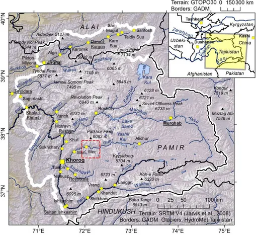
A 98 300 km2 study area in Central Asia is considered, extending from 1670 m a.s.l. near Khala-i-Khumb to 7495 m at the top of Ismoili Somoni Peak and largely corre-sponding to the headwaters of the Amu Darya River (Fig. 1). The northern and

south-10

ern boundaries of the area are formed by the Alai and Hindukush ranges in Kyrgyzstan and Afghanistan. In between, the Pamir in the Gorno-Badakhshan Autonomous Oblast of Tajikistan represents the largest share of the study area.

The western Pamir is characterized by glacierized mountain ranges exceeding 6000 m a.s.l. and deeply incised valleys. The eastern Pamir represents an arid

high-15

land above 3500 m a.s.l. with glaciers covering only the highest peaks. The more hu-mid northern Pamir with the Academy of Sciences and Transalai ranges peaks above 7000 m a.s.l. and is extensively glacierized. The Fedchenko Glacier extends over a length of>75 km and covers a surface area>700 km2.

Intense tectonic uplift in combination with glacial and fluviatile erosion

(Mah-20

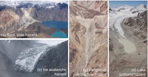
mood et al., 2008) has resulted in a particularly pronounced relief. Consequently the geomorphic activity is high, including a large variety of mass wasting processes. They are commonly triggered by earthquakes as the seismic activity and, therefore, the seis-mic hazard are significant (Giardini et al., 1999). Few large historic events such as the 1911 Sarez rock slide (Schuster and Alford, 2004; Risley et al., 2006; see Fig. 2a) or

25

(6)

NHESSD

1, 1689–1747, 2013

analysis

Title Page

Tables Figures

◭ ◮

Back Close

Full Screen / Esc

Discussion

P

a

per

|

Dis

cussion

P

a

per

|

Discussion

P

a

per

|

Discussio

n

P

a

per

|

worldwide. It retains the 60 km long Lake Sarez, the safety of which is still disputed (e.g. Risley et al., 2006).

The climate in the study area is temperate semi-arid to arid and continental with hot summers and cold winters. Most meteorological stations in the study area have recorded a positive trend of the mean annual air temperature (MAAT) in the period

5

1940–2000 (Makhmadaliev et al., 2008). The state of information suffers from a lack of up-to-date high-altitude meteorological data. According to the 4th IPCC report (IPCC, 2007), the median of the projected increase of the MAAT from 1980–1999 to 2080– 2099 for Tajikistan is 3.7◦C.

Consequently, many glaciers are retreating (e.g. Khromova et al., 2006;

Hari-10

tashiya et al., 2009; Mergili et al, 2012a), favouring the development of lakes in the glacier forefields or in subsiding areas on the glaciers. Mergili et al. (2013) detected a total number of 652 glacial lakes in the study area. A GLOF in 2002 caused dozens of fatalities, several more lakes are susceptible to sudden drainage (Mergili and Schnei-der, 2011; see Fig. 2d). Further, the retreat of glaciers over steep rock cliffs (see Fig. 2b)

15

may lead to the increased occurrence of ice avalanches. The shift of the permafrost boundary to higher areas results in the possible destabilization of rock and debris. Periglacial debris flows observed in the study area are most commonly associated with the termini of rock glaciers (see Fig. 2c).

The valleys in the study area are fairly densely populated, with Khorog as the only

20

urban centre (see Fig. 1). The local communities strongly depend on the natural re-sources and are therefore affected by the consequences of the changing temperature regime in both positive and negative ways (Kassam, 2009).

3 Data

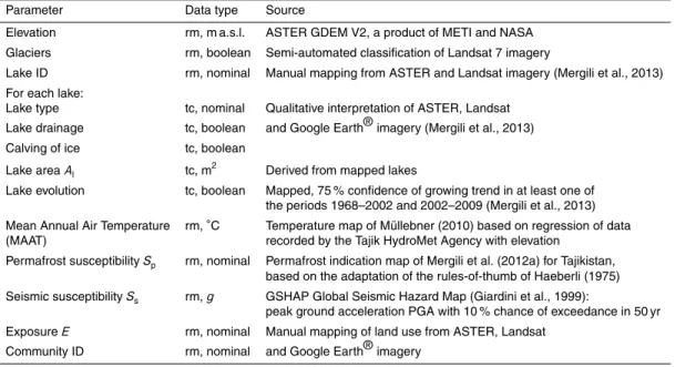
The data the high-mountain multi-risk analysis builds on are summarized in Table 1.

25

(7)

NHESSD

1, 1689–1747, 2013

analysis

Title Page

Tables Figures

◭ ◮

Back Close

Full Screen / Esc

Discussion

P

a

per

|

Dis

cussion

P

a

per

|

Discussion

P

a

per

|

Discussio

n

P

a

per

|

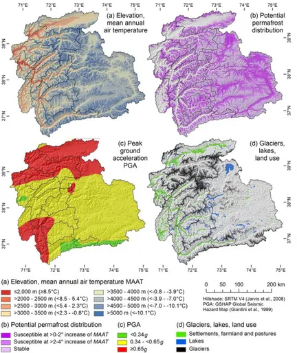
resampled to 60 m×60 m is applied. Secondary data sets such as elevation with filled sinks, slope and flow direction are generated from the DEM which is further used to generate a gridded data set of the MAAT, making use of temperature data recorded at the stations of the Tajik HydroMet Agency and a vertical temperature gradient of 0.0062◦C m−1(M ¨ullebner, 2010; Fig. 3a).

5

The identification of areas with melting permafrost builds on the permafrost indica-tion map for Tajikistan presented by Mergili et al. (2012a): a set of rules-of-thumb for the lower boundaries of sporadic and discontinuous permafrost in Switzerland (Hae-berli, 1975) is adapted to the conditions in Tajikistan. This set of rules is then combined with the DEM in order to produce a gridded dataset indicating the possibility of

per-10

mafrost occurrence for each raster cell. Applying the temperature gradient of M ¨ullebner (2010), the effects of atmospheric temperature increase on permafrost distribution are explored. Areas where the model predicts either sporadic or discontinuous permafrost for the current state, but no permafrost of either of the two types for a temperature increase of +2◦C or +4◦C, represent separate classes. Such areas are of particular

15

interest for the permafrost susceptibility scoreSp(Fig. 3b; see Sect. 4).

The seismic susceptibility of the area S_s is defined according to the peak ground acceleration with 10 % chance of exceedance in 50 yr (PGA), expressed in relation to gravityg. The Global Seismic Hazard Map (Giardini et al., 1999), an outcome of the Global Seismic Hazard Assessment Program (GSHAP), is employed (see Fig. 3c).

20

A raster map representing the glaciers in the study area is generated by a semi-automated classification of Landsat 7 satellite imagery of 2001. Three classes are dis-tinguished: debris-covered glacier, glacier with exposed ice and no glacier (see Fig. 3c). The lakes in the study area are covered by the comprehensive lake inventory presented by Mergili et al. (2013), providing detailed information on 1640 lakes (see Table 1 and

25

Fig. 3c). Besides the tabular information, a raster map with the unique ID of each lake is used.

(8)

NHESSD

1, 1689–1747, 2013

analysis

Title Page

Tables Figures

◭ ◮

Back Close

Full Screen / Esc

Discussion

P

a

per

|

Dis

cussion

P

a

per

|

Discussion

P

a

per

|

Discussio

n

P

a

per

|

cell derived by the qualitative interpretation of ASTER, Landsat and Google Earth® imagery. Table 2 shows the key used for deriving the exposure scoreE from the land use map, taking values in the range 0–4. Linear structures such as roads or power lines are not considered. Each raster cell with E >0 is associated to one of the 628 communities identified in the study area. The communities largely correspond to the

5

villages depicted in the Soviet Topographic Maps 1 : 50 000 and 1 : 100 000. However, two or more villages are grouped to one community in cases where cells with E >0 cannot clearly be assigned to one specific village.

4 Model

4.1 Concept of the multi-hazard and risk analysis

10

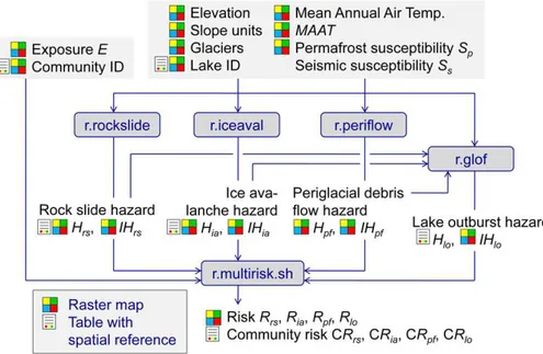
The high-mountain multi-hazard and -risk indication computer model is implemented with the Open Source software package GRASS GIS (Neteler and Mitasova, 2007; GRASS Development Team, 2013). This software builds on a flexible modular design. Simple bash scripting can be used to facilitate work flows by combining existing mod-ules. Furthermore, new modules can be added by individual developers, so that the

15

standard GIS functions are complemented by a large array of more specialized appli-cations. Such applications can be used individually or made publicly available. Exam-ples of mountain hazard models implemented with GRASS GIS include r.debrisflow (Mergili et al., 2012b), r.avalanche (Mergili et al., 2012c) and r.rotstab (Mergili et al., 2013). The model presented here builds on a combination of newly developed or

up-20

graded modules and bash scripts. The logical framework of the model is illustrated in Fig. 4, the modules dealing with the specific process types are detailed in Sects. 4.2– 4.5. The model is executed at a raster cell size of 60 m×60 m.

The high-mountain hazard analysis procedure applied at the regional scale aims at the identification of possible (i) source areas and (ii) impact areas of hazardous

25

(9)

NHESSD

1, 1689–1747, 2013

analysis

Title Page

Tables Figures

◭ ◮

Back Close

Full Screen / Esc

Discussion

P

a

per

|

Dis

cussion

P

a

per

|

Discussion

P

a

per

|

Discussio

n

P

a

per

|

hazardIH, with the exposureE there in order to derive a risk indication scoreR in the range 0–6. Table 2 shows the matrix employed for the combination ofIH andE.

The following types of processes are considered: (i) rock slides, (ii) ice avalanches, (iii) periglacial debris flows, and (iv) lake outburst floods. All of them show a potential for long travel distances and therefore represent a significant threat for the populated areas

5

in the valleys. Even though each process type is considered separately, interactions are included in the model, such as triggering of a lake outburst flood by the impact of an upslope mass movement (see Fig. 4).

The scoring scheme employed for the hazard analysis follows the same basic prin-ciple for all types of processes. It builds on susceptibility, hazard and risk indication

10

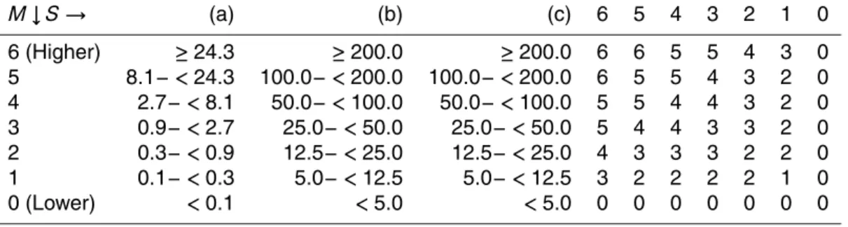
scores to be understood as ordinal numbers, not allowing for the use of arithmetic op-erations. Two-dimensional matrices are therefore used, all scores can take values in the range 0–6 (Tables 3 and 4).

The hazard indication score for the onset of a processH is computed by combining the score for the susceptibility S with the score for the expected magnitude M. The

15

susceptibility is understood as the tendency of a lake, part of a glacier or slope to produce an event and acts as a surrogate for the frequency. The expected process magnitude is based on the possible onset volume (rock slides) or on the possible onset area (ice avalanches, lake outburst floods; see Table 3).

The impact susceptibility represents the tendency of a GIS raster cell to be affected

20

by one of the considered processes. It is derived by routing the mass movement from the onset area down through the DEM. At the regional scale, empirical relationships are suitable for relating the travel distanceLor the angle of reach ωr of a flow to the involved volumeV or the peak dischargeQ_p, or for defining a global value ofω_r. The appropriate values or relationships are employed for each process type, applying the

25

(10)

NHESSD

1, 1689–1747, 2013

analysis

Title Page

Tables Figures

◭ ◮

Back Close

Full Screen / Esc

Discussion

P

a

per

|

Dis

cussion

P

a

per

|

Discussion

P

a

per

|

Discussio

n

P

a

per

|

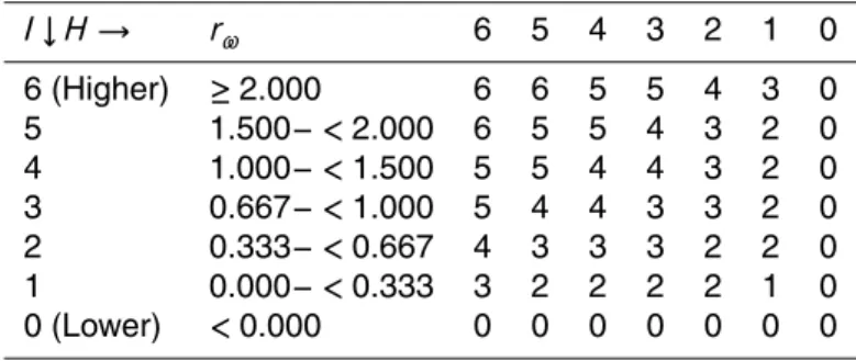
spreading. Furthermore, the linear distance from the starting point has to increase with each step of the routing procedure. For each passed cell, the average slope angle from the starting point,ω, is updated. Each random walk terminates as soon asω≤ωr,E. The impact susceptibility scoreIof each cell builds on the maximum of the ratio

r_ω=1− tanωr,A−tanω

tanω_r,A−tanω_r,E (1)

5

over all random walks.r_ω₌1 at the average angle of reach andr_ω₌0 at the lower en-velope (see Table 4).I is determined separately for each hypothetic event. The impact hazard indication scoreIH map, discretized on the basis of GIS raster cells, is derived by combiningH andI.

As the final step of the hazard analysis, the impact hazard indication scoresIH_i for

10

all hypothetic eventsi are combined in order to derive a raster map of the global hazard indication scoreIH. The maximum score is used for each raster cell:

IH₌max (IH₁,IH₂,. . .,IH_n) , (2)

where the subscripts 1, 2,. . .,nrepresent the hypothetic eventIH_i is associated with,n is the total number of possible onset areas for the considered process type.

15

Whilst the general concept outlined is applied to all types of hazards, the specific procedures for each process type are detailed in Sects. 4.2–4.5. Below, the subscript rs stands for rock slides, ia for ice avalanches, pf for periglacial debris flows and lo for lake outburst floods. Maps ofIH andR are determined separately for each process.

Given the uncertainties inherent to the regional-scale hazard and risk analysis, the

20

discretization of the results at a raster cell size of 60 m×60 m may pretend a level of detail not supported by the methodology used. According to the purpose of the study, the prioritization of target communities for risk mitigation measure, community-based risk indication scores for each process type (CRrs, CRia, CRpf, CRlo) are derived. The maxima of the raster cell-based risk indication scores over all cells representing the

25

(11)

NHESSD

1, 1689–1747, 2013

analysis

Title Page

Tables Figures

◭ ◮

Back Close

Full Screen / Esc

Discussion

P

a

per

|

Dis

cussion

P

a

per

|

Discussion

P

a

per

|

Discussio

n

P

a

per

|

to a community applies to an area<10 000 m2, CR is reduced by 1. In such cases a lower score ofR, if it applies to a larger area, may determine the score of CR for the community.

4.2 Rock slide hazard

The GRASS raster module employed for the rock slide hazard analysis is named

5

r.rockslide and, to some extent, builds on the approach of Hergarten (2012). The logical framework of r.rockslide is illustrated in Fig. 5.

Loops over all raster cells within the study area are performed separately for four as-sumptions of sliding plane inclinationβs,i(Table 5). If the local slopeβ > βs,ifor a tested cell, the cell is considered as seed cell for a possible rock slide. In order to simulate

10

a progressive failure, an inverse cone with a vertical axis and an inclination of βs,i is introduced. The apex of this cone coincides with the seed cell (see Fig. 5). All material above the cone surface (terrain elevation>cone elevation) is considered as potential rock slide material, imitating a rock slide involving all over-steepened terrain with re-spect to the base cell. For each seed cell, the volumeVrs removed by the associated

15

rock slide is recorded.

The susceptibility score S_rs for each cell with terrain elevation> cone elevation is determined according to Table 5, including the sliding plane inclinationβs,iand the per-mafrost susceptibility Sp as conditioning factors, and the seismic susceptibility Ss as possible triggering factor.S_rs can take values in the range 0–6. The rock slide hazard

20

indication scoreHrs is computed according to Table 3, with the possible event magni-tude represented by the rock slide volumeVrs. Each cell may possibly be affected by rock slides from more than one seed cell. The final hazard indication score for each raster cell is defined as the maximum ofHrs,i out of all relevant possible rock slidesi:

H_rs₌max H_rs,1,H_rs,2,. . .,H_rs,n

, (3)

25

(12)

NHESSD

1, 1689–1747, 2013

analysis

Title Page

Tables Figures

◭ ◮

Back Close

Full Screen / Esc

Discussion

P

a

per

|

Dis

cussion

P

a

per

|

Discussion

P

a

per

|

Discussio

n

P

a

per

|

The expected travel distance is estimated separately for each single possible slide (see Fig. 5), using a relationship of the type

log₁₀tanωr=alog10Vr+b, (4)

whereωr is the angle of reach andVrs is the rock slide volume. The curve has to be cut off at tanω=tanϕ, whereϕ is the angle of repose. Equation (4) is only valid as

5

long as the slide starts from rest.aand bdepend on the process type,b can also be varied in order to account for uncertainties of the relationship used. Two relationships are applied:

1. For rock slides in non-glacierized areas, the prediction curve suggested by Schei-degger (1973) is used. It was derived from a set of 33 historic and prehistoric

10

events. The correlation coefficient is 0.82, the standard deviation is 0.14298. a=−0.15666,b=0.62419 for the average and 0.36418 for the envelope.

2. It is well established that rock slides in glacierized areas often convert into rock-ice avalanches with longer travel distances (Evans and Clague, 1988; Bottino et al., 2002). If the rock slide starts in a glacierized area, or as soon as it moves over a

15

glacier, the relationship suggested by Noetzli et al. (2006) is applied:a₌−0.103, b=0.165 for the average and−0.040 for the envelope.

The steeper regression line for non-glacierized areas results in the prediction of longer travel distances by the Scheidegger (1973) model for very large volumes (V_r>361× 106m3 for the regression, V_r>34×106m3 for the envelope). This

phe-20

nomenon has no physical basis but can most likely be attributed to a lack of very large events in the data set used by Noetzli et al. (2006). In the r.rockslide model, the rela-tionship yielding the longer travel distance is used for rock slides in glacierized areas. Further, the runup height R at the opposite slope is limited by the envelope of the regression derived from the dataset presented by Hewitt et al. (2008):

25

(13)

NHESSD

1, 1689–1747, 2013

analysis

Title Page

Tables Figures

◭ ◮

Back Close

Full Screen / Esc

Discussion

P

a

per

|

Dis

cussion

P

a

per

|

Discussion

P

a

per

|

Discussio

n

P

a

per

|

100 random walks are performed for each rock slide or rock-ice avalanche, each of them starting at the highest raster cell of the hypothetic failure plane. The impact susceptibility score Irs and the impact hazard indication scoreIHrs are finally derived according to Eqs. (1) and (2) and Table 4. Equation (1) is here applied with the loga-rithms of tanω, tanω_r,Eand tanω_r,A.

5

4.3 Ice avalanche hazard

The logical framework of the ice avalanche hazard model r.iceaval is illustrated in Fig. 6. The slope beyond which glaciers or portions of glaciers are susceptible to produce ice avalanches depends on the properties of the ice which are strongly determined by the ice temperature. As data on ice temperature is not commonly available, mean annual

10

air temperature is often used as a surrogate. Huggel et al. (2004a) state that temperate glaciers produce ice avalanches at slopes above 25◦, cold glaciers at slopes above 45◦. Here, a set of 11 cases (Alean, 1985; Huggel et al., 2004a) is taken as the basis for devising a scheme for ice avalanche susceptibilityS_ia (Fig. 7). A quadratic regression is fitted for this purpose, with

15

tanβ₌3.2×10−3MAAT2−2.03×10−2MAAT₊η, (6)

whereβis the slope and MAAT is the mean annual air temperature (◦C). The intercept η=0.5555 for the regression and 0.357672 for the envelope. The thresholds applied to the ice avalanche susceptibility classesSia=0−4 are determined from Eq. (1) with η set in the way to split the data set into quartiles (see Fig. 7).S_ia is increased according

20

to the seismic susceptibility (see Table 1) so that the possible score values cover a range 0–6.

Next, clusters of cells withS_ia>0 are identified.S_iais increased by 1 for all clusters at glacier termini (no abutment). The ice avalanche hazard indication scoreHia is derived according to Table 3, combiningSia and the area of each cluster.

25

(14)

NHESSD

1, 1689–1747, 2013

analysis

Title Page

Tables Figures

◭ ◮

Back Close

Full Screen / Esc

Discussion

P

a

per

|

Dis

cussion

P

a

per

|

Discussion

P

a

per

|

Discussio

n

P

a

per

|

the travel path of ice avalanches is constrained by an average slope of 17◦, except for very large events (>5×106m3). However, such events are most commonly rock-ice avalanches or complex process chains (e.g. 1962 and 1970 Huascar ´an events, 2002 Kolka/Karmadon event), which are covered separately here, or related to volcanic pro-cesses (1980 Iliamna event, Alaska). Therefore, and since the ice avalanche volume

5

cannot be derived with the method applied, we constrain the impact area with an av-erage slope of 17◦ (tanω_r,E₌0.31). In the dataset used by Huggel et al. (2004a), the minimum value of the average slope is tanω=0.44, tanωr,Eis set to the average 0.375 andIia is computed according to Eq. (1). Equation (2) and Table 4 are applied in order to derive the ice avalanche impact hazard indication scoreIH_ia.

10

4.4 Periglacial debris flow hazard

Melting permafrost on steep slopes leaves behind a certain amount of loose debris sus-ceptible to mobilization as debris flows. Such processes may occur in the active layer, but even more where permafrost is retreating. Here, we only consider areas where re-treating permafrost is assumed (see Table 1; Mergili et al., 2012a). Figure 8 shows the

15

logical frame work of the periglacial debris flow model r.periflow. Huggel et al. (2004b) noted that, in contrast to ordinary debris flows, parameters such as slope curvature or the proximity to the stream network are hardly significant for the onset of such pro-cesses. Further, they commonly occur at slope angles from 27◦to 38◦. Table 6 shows the scheme applied here for deriving the susceptibility of each raster cell to periglacial

20

debris flowsSpfin the range from 0 to 6. We follow the findings of Huggel et al. (2004b) with regard to slope. Unfortunately, no means for the reliable distinction of bedrock and debris at the relevant scale are known to the authors. Besides slope and the state of the permafrost, the seismic susceptibility is considered for deriving Spf (see Tables 1 and 6).

25

(15)

NHESSD

1, 1689–1747, 2013

analysis

Title Page

Tables Figures

◭ ◮

Back Close

Full Screen / Esc

Discussion

P

a

per

|

Dis

cussion

P

a

per

|

Discussion

P

a

per

|

Discussio

n

P

a

per

|

commonly a rather localized process. We therefore use the approximation Hpf=Spf (see Fig. 8).

Consequently, the routing procedure (i) has to be started separately from each raster cell with Spf>0 and (ii) the average slope determining the impact area has to be in-dependent from volume. Due to the commonly large clusters of starting cells, only 10

5

random walks are started from each cell. Huggel et al. (2004b) give an envelope av-erage slope of the travel path of 11◦(tanωr,E=0.194) which is also applied here. The maximum average slope is taken from Corominas et al. (2003) who provide a value of 26◦(tanω=0.488) for debris flows<800 m³propagating on undisturbed flow paths assumed for the study area. The average of the two values, 0.341, is taken as tanωr,A.

10

I_pf is computed according to Eq. (1). ForI_pf<4, the runup on the opposite slope is re-stricted. Equation(2) and Table 4 are applied to derive the periglacial debris flow impact hazard indication scoreIH_pf.

4.5 Lake outburst hazard

An improved version of the GRASS GIS raster module r.glof (Mergili and Schneider,

15

2011) is used for the lake outburst hazard analysis. The logical framework of r.glof is illustrated in Fig. 9.

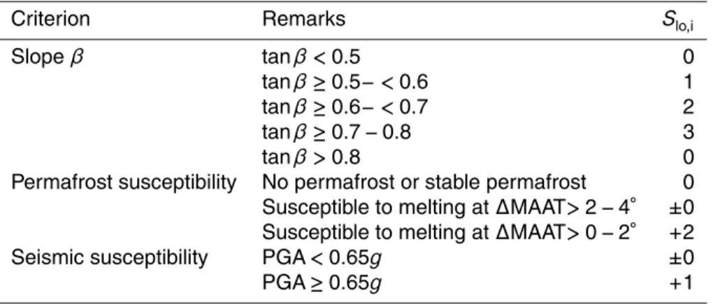
First, the susceptibility scores for (i) lake outburst caused by internal factors (dam failure)Slo,i and (ii) lake outburst triggered by external factors (impact of mass move-ments)Slo,eare considered separately (see Fig. 9).Slo,iandSlo,ecan take values in the

20

range 0–6, negative values are set to 0.

The derivation ofSlo,ibuilds on the following key parameters: (i) lake type, indicating the dam material; (ii) mode of lake drainage; (iii) lake evolution; (iv) dam geometry; (v) permafrost susceptibility; (vi) seismic susceptibility (see Table 1). Table 7 shows the scoring scheme applied. The lake type (Mergili et al., 2013) is taken as basis, with

25

(16)

NHESSD

1, 1689–1747, 2013

analysis

Title Page

Tables Figures

◭ ◮

Back Close

Full Screen / Esc

Discussion

P

a

per

|

Dis

cussion

P

a

per

|

Discussion

P

a

per

|

Discussio

n

P

a

per

|

an idealized average downstream slope of the dam: the dam widthW is defined as the Euclidean distance between the lake outlet and the closest raster cell along the downstream flow path with a lower elevation than the average lake bottom, using the average lake depthDlaccording to Huggel et al. (2002):

Dl=1.04×10−1A0.42_l , (7)

5

whereA_l is the lake area (m2),D_l is given in m. The tangent of the average slope of the dam in outflow direction, tanβd, is derived asDl/W. For very gentle downstream average slopes tanβd<0.02,Slo,iis decreased by 1 (see Table 7).

The event at Laguna 513 in the Cordillera Blanca (Haeberli et al., 2010b) has shown the need to include the entire catchment when analyzing lake outburst susceptibility.

10

The topographic susceptibility TS is introduced in order to account for this need, em-ploying the impact hazard indication scores for rock slidesIH_rs, for ice avalanchesIH_ia, for periglacial debris flowsIH_pf, and for outburst floods of lakes in the upper catchment IH_lo. The overall maximum score over the raster cells representing the considered lake (IH_ia,max, IH_rs,max, IH_pf,max, and IH_lo,max) applies, but the impact of periglacial debris

15

flows and upstream lake outburst floods is down-weighted:

TS₌max IH_rs,max,IH_ia,max,IH_pf,max−3,IH_lo,max−3

. (8)

The topographic susceptibility is taken as the basis for the rating of the susceptibility to lake outburst triggered by external factorsSlo,e. If direct calving of ice into the lake is possible, the score forSlo,eis set to a minimum of 3.

20

The maximum of S_lo,i and S_lo,e is used as lake outburst susceptibilityS_lo. S_lo is re-duced for lakes with a high freeboardF (defined as the difference between the DEM with filled sinks and the original DEM for the lake centre): for lakes withF >50 m the score is decreased by 3. For lakes with F >25 m it is decreased by 2, and for lakes withF >10 m, the score is decreased by 1 in order to derive the final value ofSlo.

25

(17)

NHESSD

1, 1689–1747, 2013

analysis

Title Page

Tables Figures

◭ ◮

Back Close

Full Screen / Esc

Discussion

P

a

per

|

Dis

cussion

P

a

per

|

Discussion

P

a

per

|

Discussio

n

P

a

per

|

Possible outburst floods are routed downwards through the DEM separately for each lake, the travel distance is determined according to the relationships listed in Table 8. After the deposition of the debris or mud, or if not much sediment is entrained at all, the flood may propagate much farther: Haeberli (1983) suggests an average angle of reach of 2−3◦, but also travel distances exceeding 200 km are reported (e.g. Hewitt,

5

1982).

In order to achieve a robust estimate of the travel distance, the impact area of possi-ble lake outburst floods and, consequently, the impact susceptibilityI_lo, the approaches T1–T4 shown in Table 8 are combined (Eq. 1 is not applied for lake outburst floods). The lake outburst flood is routed down starting from the outlet of the considered lake.

10

800 random walks are performed for each lake. A random walk is forced to terminate if it impacts a larger lake.

For T1, the debris flow volumeVdis set to five times the outburst volume (maximum sediment concentration in steep flow channels∼80 % according to Iverson, 1997) in order to account for sediment bulking. The outburst volume is set to the entire lake

15

volume, lake areaAl multiplied with lake depthDl). For T2, we use an angle of reach ω_r=8◦ which is most likely more suitable for the study area (Mergili and Schneider, 2011) thanωr=11

◦

as suggested by Haeberli (1983). Several authors have introduced empirical relationships for relating the peak dischargeQp (m

3

s−1) – required as input for the relationship T3 in Table 8 – to the outburst volume and the dam height (Costa,

20

1985; Costa and Schuster, 1988; Walder and O’Connor, 1997; Table 9). Qp is deter-mined from the maximum of the results computed with the relationships Q1–Q6 shown in Table 9. T1 and T3 are only applied to glacial lakes as there is no basis available for calculating the depth or volume of lakes assigned to the other types. Instead, the angle of reach is set toωr=11

◦

(the value suggested by Haeberli, 1983) for T1 and to

25

ωr=14 ◦

for T3.

(18)

NHESSD

1, 1689–1747, 2013

analysis

Title Page

Tables Figures

◭ ◮

Back Close

Full Screen / Esc

Discussion

P

a

per

|

Dis

cussion

P

a

per

|

Discussion

P

a

per

|

Discussio

n

P

a

per

|

the opposite slope is restricted. If only an impact as flood is predicted, (T4;Ilo≤3), the impact susceptibility is further di_fferentiated according toω: forω≥6,Ilo=3, forω≥4, Ilo=2 and forω≥2,Ilo=1. T4 is only applied to lakes≥50 000 m

2

. Furthermore, the criterion that the distance from the source has to increase with each computing step is disabled for floods.

5

In an analogous way to the scores for the rock slides, ice avalanches and periglacial debris flows (see Sections 4.2–4.4), the impact hazard indication score is then derived by combiningI_lo with H_lo of the corresponding lake (see Table 4). The global impact hazard indication score IH_lo of a given raster cell is defined as the maximum of all lake-specific scores (see Eq. 2).

10

5 Results

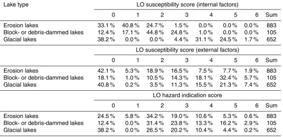
The total area with significant periglacial debris flow (PF) susceptibility/hazard is much larger than those for the other hazard types: 9.9 % of the entire study area are des-ignated as possible PF source areas, based on the criteria defined in Table 6. 42.7 % out of this area are assigned the three higher susceptibility scores 4–6 (Fig. 10a). This

15

pattern indicates the ubiquity of hazardous areas on the one hand, but also the lim-ited means of a sharper delineation on the other hand. In contrast, the ice avalanche (IA) susceptibility and the lake outburst (LO) susceptibility, due to their confinement to glaciers and lakes, respectively, are constrained in a much sharper way. 1.6 % of the total study area are identified as susceptible to IA, 64.5 % out of this area are assigned

20

the susceptibility scores 4–6 (see Fig. 10a). The LO susceptibility is discretized on the basis of lakes. 70.9 % of all lakes are assigned susceptibility scores >0, 50.0 % of these lakes the susceptibility scores 4–6 (see Fig. 10a). The rock slide (RS) suscepti-bility displays intermediate patterns in terms of the total area identified as susceptible (4.7 % of the total study area). However, only 16.2 % of this area – a much lower value

25

(19)

NHESSD

1, 1689–1747, 2013

analysis

Title Page

Tables Figures

◭ ◮

Back Close

Full Screen / Esc

Discussion

P

a

per

|

Dis

cussion

P

a

per

|

Discussion

P

a

per

|

Discussio

n

P

a

per

|

scores 4–6 (see Fig. 10a). The reason for this phenomenon is the limited area occu-pied by very steep slopes (see Table 5).

The distribution of the raster cells or lakes identified as susceptible among the six hazard indication score classes is illustrated in Fig. 10b, depending on the susceptibility and the possible process magnitude (see Table 3). 38.1 % of the RS and 68.4 % of

5

the IA are assigned the hazard indication scores 4–6. In the case of PF, hazard and susceptibility are identical due to lacking means for an estimation of the magnitude (see Sect. 4.4). Comparatively few lakes (23.9 %) are assigned the LO hazard indication scores 4–6. This phenomenon is explained by the large number of rather small but highly susceptible lakes.

10

Figure 11 represents the hazard indication scores for each process type broken down to the level of small catchments identical to the output parameter basin of the GRASS GIS raster module r.watershed (GRASS Development Team, 2013) with a threshold parameter of 5000. The maximum out of all raster cell-based hazard indication scores is shown for each catchment, except for the LO hazard where the value assigned to

15

each lake is illustrated.

As expected, the RS hazard (see Fig. 11a) is highest in areas with a particularly steep topography in the northern and central Pamir. More localized high-hazard ar-eas are distributed throughout the study area. The IA hazard (see Fig. 11b) is high in most glacierized areas (see Fig. 3d), particularly in parts of the northern Pamir where

20

large portions of steep glaciers are extremely abundant. Within these zones the inter-catchment differentiation of hazardous areas is rather poor.

The PF hazard is poorly differentiated at the catchment scale: steep slopes near the permafrost boundary are almost ubiquitous in the study area (see Fig. 3b), except for the elevated and comparatively gently inclined south eastern portion. The most

no-25

(20)

NHESSD

1, 1689–1747, 2013

analysis

Title Page

Tables Figures

◭ ◮

Back Close

Full Screen / Esc

Discussion

P

a

per

|

Dis

cussion

P

a

per

|

Discussion

P

a

per

|

Discussio

n

P

a

per

|

could help to sharpen the distinction between more and less hazardous areas. How-ever, as rock glaciers are extremely common throughout the study area, the patterns at the inter-catchment level would most likely remain unchanged.

As the LO hazard is directly related to the well-known lake distribution it can be dis-cretized at a high level of detail (see Fig. 11d). Nine lakes are assigned the highest

5

LO hazard indication scoreHlo=6, the largest of them is Lake Sarez. Even though – or because – the safety of Lake Sarez is highly disputed (e.g. Risley et al., 2006), this classification seems reasonable. The LO susceptibility scoreS_lo=5 is a consequence of the high topographic susceptibility. The same is true for Lake Zardiv, with 0.7 km2 the second largest lakes withHlo=6 (see Fig. 11d). Further lakes of interest are, e.g.

10

Lake Khavraz and Lake Shiva. Lake Khavraz is an 1.9 km2 lake impounded behind a rock glacier at an elevation of 4000 m a.s.l., in the zone of possibly melting permafrost. Here both the topographic susceptibility (Slo,e=5) and the LO susceptibility due to in-ternal factors (S_lo,i=5) are at high levels. Lake Shiva is assigned a susceptibility in the medium range of the scale (Slo=3) and a sudden drainage is not likely but, due to the

15

large size of 15.2 km2,Hlo=5. The lake is located close to several communities in the Panj Valley which could be affected in the case of such an event. The largest lake in the study area, Kara Kul, is assigned a hazard indication score of 4 (see Fig. 11d). The LO susceptibility of Kara Kul is rated with a score ofSlo=2, only the very large lake area (405 km2) leads to the relatively high hazard indication score. The fact that a closer

20

look reveals no significant outburst hazard of Kara Kul suggests that the approach used tends to overestimate the hazard for large lakes. One reason for this phenomenon is the topographic susceptibility: large lakes have the ability to alleviate the impact of mass movements rather than small lakes. However, an objective basis to include the dependence of the topographic susceptibility on lake size is missing. Table 10

sum-25

(21)

NHESSD

1, 1689–1747, 2013

analysis

Title Page

Tables Figures

◭ ◮

Back Close

Full Screen / Esc

Discussion

P

a

per

|

Dis

cussion

P

a

per

|

Discussion

P

a

per

|

Discussio

n

P

a

per

|

The median and maximum travel distances computed for each process type are summarized in Table 11. The RS model commonly predicts travel distances of 3.0 km (average)–5.6 km (envelope), but for very large events (>800×106m3) extending over vertical distances >4000 m the model, when applied with the envelope, predicts a travel distance of almost 50 km (see Eq. 4). The IA model (ω_r,E₌17◦) and the PF model

5

(ωr,E=11 ◦

) predict shorter travel distances. Note that, in both cases, the difference between the median and the maximum is only caused by topography and not by the assumed process magnitude. The LO model predicts the possibility of a significant debris flow for less than half of all lakes (no meaningful median value can therefore be given in Table 11). The reason for this phenomenon is mainly the gentle slope observed

10

downstream from many lakes. However, lakes with steeper downstream slopes can produce debris flows with travel distances>15 km and floods >80 km, according to the model.

Figure 12 shows the distribution of the impact hazard. For clarity, only the raster cell values along the main flow channels are shown. It is clear that the general patterns of

15

the impact hazard at the broad scale resemble those of the hazard shown in Fig. 11: whilst a possible impact of rock slides and periglacial debris flows is shown for most valleys particularly in the western part of the study area (Figs. 12a and 12c), a more localized impact of ice avalanches and lake outburst floods is suggested by the model (Figs. 12b and 12d).

20

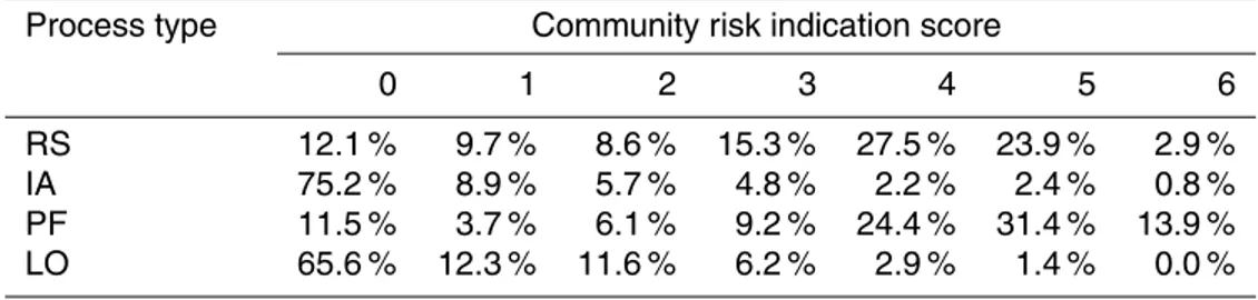
The distribution of community risk over the study area reflects the patterns shown in Figs. 11 and 12 on the one hand, and the distribution of the exposed communities on the other hand. Figure 13 illustrates the relative frequency of the community risk indi-cation score classes for 15 regions within the study area, each of them representing a catchment or section of a catchment. The eastern Pamir is considered as one single

25

(22)

NHESSD

1, 1689–1747, 2013

analysis

Title Page

Tables Figures

◭ ◮

Back Close

Full Screen / Esc

Discussion

P

a

per

|

Dis

cussion

P

a

per

|

Discussion

P

a

per

|

Discussio

n

P

a

per

|

middle Panj valleys as well as in the Gunt Valley (see Fig. 13a). The hot spots of ice avalanche risk are identified in the Vanch and Bartang valleys, both deeply incised into glacierized mountain ranges (see Fig. 13b). This type of risk plays a less promi-nent role in the other regions. Also the risk of periglacial debris flows is highest in the deep gorges of the western Pamir, decreasing towards north where permafrost is less

5

abundant (see Fig. 13c). However, the model predicts a significant PF risk for most communities throughout the study area. This is not the case for the risk caused by lake outburst floods, which is significant mainly in the south western Pamir and in part of the northern Pamir (see Fig. 13d). The LO community risk indication score CRlo=6 is not assigned to any village. Table 12 summarizes the relative frequency of villages

10

assigned to each class with respect to all four hazard types.

A composite hazard and risk indication map is prepared for the entire study area. It provides a visual overlay of the hazard, impact hazard and community-based risk indication scores for each of the four process types considered in the study. Figure 14 shows this map for a selected area covering the Gunt Valley and its tributaries (see

15

Fig. 1 for delineation). The area affected by the prehistoric Charthem rock slide (see Fig. 14a) is very well reproduced by the model, therefore a high RS risk is assigned to the nearby communities. However, also several other communities and lakes are pos-sibly impacted by rock slides. The patterns of IA hazard and risk illustrate the isolated appearance of this type of hazard in the area (see Fig. 14b). Even though the main

20

effect of the process is the possible impact on lakes, some communities in the main valley are at risk, but assigned rather low scores. Areas of PF hazard (see Fig. 14c) are strictly confined to steep slopes near the permafrost boundary which are however very common along the slopes of most valleys, confirming the broad-scale patterns shown in Fig. 11c. Therefore, most of the communities in the valleys are identified as at risk.

25

(23)

NHESSD

1, 1689–1747, 2013

analysis

Title Page

Tables Figures

◭ ◮

Back Close

Full Screen / Esc

Discussion

P

a

per

|

Dis

cussion

P

a

per

|

Discussion

P

a

per

|

Discussio

n

P

a

per

|

Several lakes have developed near the termini of the glaciers of the tributary val-leys (Mergili and Schneider, 2011; Mergili et al., 2013). Three of them are assigned the hazard indication score Hlo=5 (see Fig. 14d). The debris flow travel distances predicted by the LO model are relatively short, only debris flows from two lakes could reach the communities of the main valley: the village of Varshedz is just located at the

5

terminus of a possible debris flow starting from Lake Varshedz (see Fig. 2d; lake area 0.16 km2,S_lo=5,H_lo=5). Lake Nimats, an erosion lake withS_lo=4 andH_lo=5, drains into a very steep channel heading directly down to the main valley. In the case of a (not very likely) sudden drainage, the nearby villages would most likely suffer substantial damage. The impact area of the distal floods resulting from the possible drainage of

10

Lake Varshedz or Lake Nimats is characterized by lower to medium community risk indication scores of the possibly affected villages. The largest lake shown in Fig. 14d is Rivakkul (1.2 km2,Slo=4,Hlo=5). It is characterized by a very gently inclined down-stream valley. As a result, the model predicts only a comparatively short travel distance of a possible outburst flood (4.6 km), being alleviated far upslope from the villages in

15

the main valley.

6 Discussion

The purpose of the model approach introduced in the previous sections and the re-sulting hazard and risk indication maps is to provide a reproducible basis for targeted hazard and risk assessment studies and mitigation measures at the community scale.

20

The approach chosen is thought to be useful for the study area in the Pamir for two reasons.

First, the general di_fficulty of establishing frequencies for rare or singular events in combination with sparse historical data in the study area makes strictly quantitative approaches such as statistical methods inapplicable. Therefore a hazard and risk

in-25

(24)

NHESSD

1, 1689–1747, 2013

analysis

Title Page

Tables Figures

◭ ◮

Back Close

Full Screen / Esc

Discussion

P

a

per

|

Dis

cussion

P

a

per

|

Discussion

P

a

per

|

Discussio

n

P

a

per

|

Second, the vulnerability of the local population to these types of hazards is high, even though NGOs have launched programs to improve the awareness of and the pre-paredness for geohazard events in the previous decade. This situation is comparable to other high-mountain areas in developing countries (e.g. Carey, 2005). The results of the present study shall highlight high-risk areas and serve as a baseline for in-detail

5

studies and risk mitigation procedures.

Consequently, the outcome of the study should not be seen as definite hazard and risk maps, but rather as conceptual hazard and risk indication maps. The hazard and risk indication score classes are therefore not given definite names such as Moderate hazard, Extremely high risk etc. Further, the interpretation of the model results on the

10

basis of raster cells is appropriate for scientific discussion, but not for the design of risk mitigation measures. Here the scale of communities (see Fig. 14), catchments (see Fig. 12) or even regions (see Fig. 13) are much more suitable.

As far as a comparison with observed events is possible, it confirms the model results (e.g. Charthem rock slide, see Fig. 14a). In the case of large rock slides such as the

15

1911 Sarez event (see Fig. 2a) the comparison with the model results is of limited value due to the substantial change of the topography caused by such events. No records of ice avalanches in the study area are known to the authors whilst periglacial debris flows are very common. Their source and impact areas are well recognized by the model, but the false positive rate is high. The two lakes with recorded sudden drainage

20

are not characterized by exceptionally high susceptibility scores – the prediction of lake outburst floods is therefore particularly challenging.

The quality of the model results strongly depends on the input data used. The de-tail and accuracy of the ASTER GDEM is considered sufficient for the purpose of the present study, even though the quality of the dam geometry estimates may suffer from

25

(25)

NHESSD

1, 1689–1747, 2013

analysis

Title Page

Tables Figures

◭ ◮

Back Close

Full Screen / Esc

Discussion

P

a

per

|

Dis

cussion

P

a

per

|

Discussion

P

a

per

|

Discussio

n

P

a

per

|

predicted conditions and scenarios are likely to be realistic, uncertainties are hard to quantify. The seismic hazard map used (Giardini et al., 1999) is a highly generalized global dataset. Other essential information such as the distinction bedrock – residual rock or the orientation and dip of the bedding planes of geological layers are hardly manageable at the scale relevant for a study of this type.

5

The scoring schemes used (see Tables 2–7) are founded on expert knowledge. The interpretation of the model results have to consider the characteristics of the scheme used for each process. Necessarily, the schemes contain±arbitrary thresholds such as those used for the event magnitude (see Table 3) or the 45◦minimum slope for rock slides already used earlier by Hergarten (2012).

10

The modelling of the travel distance and the impact area of the considered processes is derived from the statistics of observed events. These statistics are reasonably robust for rock slides and rock ice avalanches (Scheidegger , 1973; Evans and Clague, 1988; Bottino et al., 2002; Noetzli et al., 2006) and also for ice avalanches (Huggel et al., 2004a). However, they are based on observations from other mountain areas such as

15

the Alps. Their application is based on the hypothesis that (i) the patterns observed there are comparable to those in the Pamir and (ii) that the – often rather small – datasets used for the derivation of the patterns and thresholds cover a representative sample of the reality. This is equally true for the slope-temperature curve shown in Fig. 7. The situation is even more difficult for periglacial debris flows (Huggel et al.,

20

2004a) and particularly for lake outburst floods. The threshold of ωr,E=11 ◦

used by Huggel et al. (2004a, b) for debris flows from lake outburst events is not applicable to the Pamir as the 2002 Dasht event, whereωr,E∼9.3

◦

, has shown (Mergili and Schnei-der, 2011). Also the parameterization of floods developing from lake outburst events is nothing more than a rough estimate so that the results (such as the short travel

dis-25

tance predicted for a sudden drainage of Rivakkul, see Fig. 14d) have to be interpreted with utmost care.

(26)

NHESSD

1, 1689–1747, 2013

analysis

Title Page

Tables Figures

◭ ◮

Back Close

Full Screen / Esc

Discussion

P

a

per

|

Dis

cussion

P

a

per

|

Discussion

P

a

per

|

Discussio

n

P

a

per

|

paths. The criterion that the motion has to move away from the source with each step of the random walk partly accounts for this limitation.

Possible impact wave due to mass movements into lakes are explicitly accounted for by the model. Other types of interactions are included indirectly: the conversion of rock slides into rock-ice avalanches by the impact on glaciers is implicitly considered in the

5

rock slide model, even though there are no means to estimate the entrainment of snow or ice. In the case of rock slides and rock-ice avalanches, the empirical relationships used implicitly include cascading e_ffects such as the conversion into debris flows. Some process interactions are out of scope of the present study, such as the damming of lakes by mass movements and possible subsequent drainage. The same is true for the

10

entrainment of debris, modelling of which remains a challenge particularly at the scale of the present study.

The approach used does not allow for an analytical overlay of the susceptibility, haz-ard, impact hazard and risk indication scores associated to each process type. Even though attempted as far as possible, a homogenization of the scoring schemes for the

15

different processes proves highly problematic due to the missing physical basis. The data the analysis is based on differs between the processes: e.g. the possible mag-nitude of rock slides is given in maximum volumes whilst only the maximum involved surface area allowed under the assumptions taken is used for possible ice avalanches and lake outburst floods (see Table 3). Also the schemes for susceptibility can hardly

20

be homogenized (see Tables 5–7; Fig. 7), partly due to the varying level of detail of the available input data.

7 Conclusions

A regional-scale multi-hazard and -risk indication model was introduced, including four selected high-mountain processes: (i) rock slides and rock avalanches, (ii)

ice-25

(27)

NHESSD

1, 1689–1747, 2013

analysis

Title Page

Tables Figures

◭ ◮

Back Close

Full Screen / Esc

Discussion

P

a

per

|

Dis

cussion

P

a

per

|

Discussion

P

a

per

|

Discussio

n

P

a

per

|

The model shall help to distinguish areas with higher from those with lower risk, even though the possibilities for comparison with observed events are limited. The inter-pretation of the model results – preferably at the level of communities, catchments or regions – has to take into account the characteristics of the scoring schemes as well as the limitations of the input data and the methodology used.

5

Acknowledgements. The work presented is part of the project PAMIR supported by the

Eu-ropean Commission (EC) and the Austrian Development Agency (ADA), as well as of the project TajHaz supported by FOCUS Humanitarian Assistance (an affiliate of the Aga Khan Development Network), the Swiss Agency for Development and Cooperation (SDC) and the UK Department for International Development (DFID). The Tajik Agency of Hydrometeorology

10

has provided meteorological data. Special thanks for their support go to Matthias Benedikt, Johannes P. M ¨uller and Jean F. Schneider, BOKU University, Vienna.

References

Alean, J.: Ice avalanches: some empirical information about their formation and reach, J. Glaciol., 31, 324–333, 1985.

15

Beniston, M.: Climatic Change in Mountain Regions: A Review of Possible Impacts, Clim. Change, 59, 5–31, doi:10.1023/A:1024458411589, 2003.

Bolch, T., Peters, J., Yegorov, A., Prafhan, B., Buchroithner, M., and Blagoveshchensky, V.: Identification of potentially dangerous glacial lakes in the northern Tien Shan, Nat. Hazards, 59, 1691–1714, doi:10.1007/s11069-011-9860-2, 2011.

20

Bottino, G., Chiarle, M., Joly, A., and Mortara, G.: Modelling Rock Avalanches and Their Rela-tion To Permafrost DegradaRela-tion in Glacial Environments. Permafrost Periglac., 13, 283–288, doi:10.1002/ppp.432, 2002.

Breien, H., DeBlasio, F. V., Elverhoi, A., and Hoeg, K.: Erosion and morphology of a de-bris flow caused by a glacial lake outburst flood, Western Norway, Landslides, 5, 271–280,

25

doi:10.1007/s10346-008-0118-3, 2008.