Exploiting item co-utility to improve recommendations

(1)

EXPLOITING ITEM CO-UTILITY

(2)

(3)

ALINE BESSA

EXPLOITING ITEM CO-UTILITY

TO IMPROVE RECOMMENDATIONS

Dissertation presented to the Graduate Program in Computer Science of the Fed-eral University of Minas Gerais in partial fulfillment of the requirements for the de-gree of Master in Computer Science.

Advisor: Nivio Ziviani

Co-Advisor: Adriano Veloso

Belo Horizonte

(4)

Bessa, Aline Duarte

B557e Exploiting item co-utility to improve recommendations / Aline Duarte Bessa.— Belo Horizonte, 2013.

xiii, 49 f.: il.; 29 cm.

Dissertação (mestrado) — Universidade Federal de Minas Gerais. Departamento de Ciência da Computação.

Orientador: Nívio Ziviani.

Coorientador: Adriano Alonso Veloso.

1. Computação - Teses. 2. Sistemas de

recomendação

– Teses. 3. Recuperação da informação – Teses. I..Orientador. II. Coorientador. III. Título.

(5)

(6)

(7)

To Raja and Lico.

(8)

(9)

Acknowledgments

First to my advisor, Nivio Ziviani, who supported me throughout this process. I would also like to especially thank Adriano Veloso, for being a dedicated co-advisor. Looking back over the past two years I have learned undeniably much, thanks to these two professors in particular, but also to UFMG in general. I also thank professor Juliana Freire from NYU-Poly, who held an advisory role for me during my internship in 2013 and substantially changed my viewpoints on how to perform research.

Most of this thesis would not have been possible without the fruitful suggestions of my colleagues. First Filipe Arcanjo, who helped me on understanding the relevance of what I was studying, and on whom I bounced ideas since my first months in Belo Horizonte. Special thanks to Fernando Mourão, who have given me substantial ideas for experiments and validation. I have learned much from my peers at LATIN: Aé-cio Santos, Adolfo Guimarães, Wladmir Brandão, Thales Costa, Cristiano Carvalho, Arthur Camara, Anisio Lacerda, Sabir Ribas, and Leonardo Resende; and at NYU-Poly: Fernando Chirigati, Tuan-Anh, and Kien Pham. I also would like to thank CNPQ and CAPES for funding my research.

If not for friends, I would not have had enough motivation to go through my master’s. I would like to thank Denise Neri, Fernanda Wanderley, Roy Hopper, and Anthony Farnham for supporting me in so many ways during my time in Belo Horizonte and New York City. To my old yet always present friends, Clara Fernandes, Julianna Oliveira, Amine Portugal, Renata Amoedo, Rafael Saraiva, Alexandre Passos, thanks for hitting me up constantly through Skype and e-mails, you are all very important to me.

I also thank my family, Marcia Bessa, Andrea Bessa, and Adriano Bessa, who have inspired me and taught me how to stay strong even when I think I cannot.

And last, but not least, I want to thank Davi, my love and best friend, for reviewing this work and giving me invaluable advice and support all the time.

(10)

(11)

“Life is the sum of all your choices.” (Albert Camus)

(12)

(13)

Abstract

In this thesis, we consider that a recommendation was useful if the associated user’s feedback was positive – e.g., the user purchased the recommendation, gave it a high rating, or clicked on it. We then formalize the concept of co-utility, stated as the property any two items have of being useful to a user, and exploit it to improve recom-mendations. We then present different ways of estimating co-utility probabilities, all of them independent of content information, and compare them with each other. We embed these probabilities, as well as normalized predicted ratings, in an instance of an

N P −hardproblem named Max-Sum Dispersion Problem. A solution to this problem

corresponds to a set of items for recommendation. We study two heuristics and one exact solution to the Max-Sum Dispersion Problem and perform comparisons among them. According to our experiments, the three solutions have similar performance in practice. We also contrast our method to different baselines by comparing the ratings users give to different recommendations. We obtain expressive gains in the utility of recommendations, up to 106%, and our method also recommends higher rated items to the majority of users. Finally, we show that our method is scalable in practice and does not seem to affect recommendations’ diversity.

Keywords: Recommender Systems, Co-Utility, Max-Sum Dispersion Problem.

(14)

(15)

Chapter 1 Introduction

People from widely varying backgrounds are inundated with options that lead to a situation known as “information overload”, where the presence of too much informa-tion interferes with decision-making processes [Toffler, 1970]. To circumvent it, content providers and electronic retailers have to identify a small yet effective amount of infor-mation that matches users’ expectations. In this scenario, Recommender Systems have become tools of paramount importance, providing a few personalized recommendations that intend to suit user needs in a satisfactory way.

One type of such systems, known as Collaborative Filtering, makes predictions about the interests of a user by gathering taste information from many other users. It generally works as follows: (i) prediction step - keeps track of users’ known preferences and processes them to predict items that may be interesting to other users; (ii) rec-ommendation step - selects predicted items, optionally ranks them, and recommends them to users [Adomavicius and Tuzhilin, 2005]. The scope of this work is limited to Collaborative Filtering. We also do not perform ranking, and therefore do not analyse the impact that the order of items may have on recommendations.

In the prediction step, scores are independently assigned to items by taking user’s historical data into account [Ricci et al., 2011]. The higher the score the higher the estimated compatibility between the item and user’s known preferences. It is therefore intuitive to think that the highest scored items should be the ones selected in the recommendation step. This is indeed what happens in the recommendation step of many systems, where the selection of items is based exclusively on how well they match users’ known preferences. Nonetheless, by neglecting relations between predicted items, such systems may generate less useful recommendation lists. A large body of research, dating back from early studies in the 1960s, draws attention to the importance of exploiting dependencies between items [Bookstein, 1983; Carbonell and Goldstein, 1998].

(18)

2 Chapter 1. Introduction

In this work, we focus on improving the utility of recommendations by exploiting relations between items. In our case, the relation in question is co-utility, and other examples of item relations are diversity or competition [Zhang and Hurley, 2008; Xiong et al., 2012]. Throughout this work, we consider that a recommendation was useful if the associated user’s feedback was positive – e.g., she purchased the recommendation, gave it a high rating, or clicked on it. Breese et al. [1998] and Passos et al. [2011] also relate utility to positive feedback – high ratings, in particular. With respect to relations between items, we focus on their co-utility, a concept that is defined in the following.

Definition 1. Two items are co-useful with respect to a user if she considered both of them useful. Co-utility is the property of being co-useful.

For each pair of items, we compute their probabilities of being co-useful, as de-tailed in Chapter 3, and embed this information into methods designed to generate recommendations. As we explain in Chapter 2, other works exploit relations between items for recommendations, especially when they account for diversity. Nonetheless, to the best of our knowledge, our work is the first to address co-utility relations in the context of items’ recommendation.

This work is motivated by the Theory of Choice of Amos Tversky [Tversky, 1972], which indicates that preference among items depends not only on the items’ specific features, but also on the presented alternatives. In our case, the selection of an item is based on its independently predicted rating and on how likely it is to be co-useful with other selected items. The simplicity of estimating co-utility probabilities and the fact that they are underexploited in the literature to date were also important motivations behind this work.

1.1 Work Contributions

Some of the specific contributions of this work include:

• A definition of co-utility and methods for estimating co-utility probabilities. Such methods are time efficient and do not depend on content information.

(19)

1.2. Research Development 3

• A thorough evaluation of our method. We compare different algorithms that adopt co-utility probabilities with methods that neglect relations between items and with methods that take them into consideration. Our comparisons are mainly focused on recommendations’ utility, albeit we briefly address diversity as well.

• An analysis of the scalability of our method, which indicates that it is applicable for real-world recommender systems.

1.2 Research Development

This informal description aims to help you, the reader, understand the trajectory of this work. We portray not only the choices that led to the theme of this dissertation but also our main difficulties.

This research started as a study on diversity in the context of recommender systems. The abundance of work in this area, alongside the fact that it is hard to understand to what extent diversity should be regarded [Pu et al., 2012], has motivated us to focus on other types of relation between items. The idea of modelling co-utility probabilities came up naturally, and after a thorough investigation we concluded that it was rather original in our context.

Initially, we combined co-utility probabilities and predicted scores in a bayesian fashion. The selection of an item for recommendation depended on its prior probability of being useful, and its posterior probability of being useful given the items that were already selected for recommendation. For example, the selection of the first item, i1,

depended on its prior probability; the selection of the second item, i2, depended on its

prior probability and on its posterior probability given that i1 was selected etc. These

prior probabilities were straightforward normalizations of predicted scores, and the posterior probabilities were computed as co-utility probabilities.

(20)

4 Chapter 1. Introduction

practical enough due to slow convergence, and we were not convinced as to whether it would work in real-time situations.

Some time later, we noticed that we could linearly combine predicted scores and co-utility probabilities, pose the combination as an optimization problem, and then tackle it under an Operations Research paradigm. Our combination trivially reduced to a Facility Location Analysis problem named Max-Sum Dispersion Problem [Borodin et al., 2012]. We detail the connection between our work and Max-Sum Dispersion Problem in Chapters 2, 3, and 4.

After the definition of our optimization problem, we performed experiments to analyse if the exploitation of co-utility probabilities could improve recommendations’ utility. Although we were no longer focusing on diversity, we did not want to generate redundant recommendations, so our experiments also analysed whether our recommen-dation lists were redundant. Finally, we studied the scalability of our method.

The results of these experiments, and comparisons with different baselines, were published as a full-paper in SPIRE 2013, namely Bessa et al. [2013]. By that time, co-utility probabilities bore the name ofmutual influence, but after SPIRE we concluded that this term was not very accurate. After SPIRE 2013, we studied more algorithms to the Max-Sum Dispersion Problem, a different way of estimating co-utility probabilities, and ran more experiments. Throughout this entire research, we had a difficulty with the choice of baselines, as we explain in Chapter 2. Albeit some of them were recommended by SPIRE reviewers and other researchers, we still think it would be better if at least one of them addressed co-utility in a way that is similar to ours.

1.3 Work Outline

The remainder of this work is organized as follows.

Chapter 2 [Related Work] Related work is discussed and connected to our study.

Chapter 3 [Basic Concepts] Basic definitions, notations, and functions concerning our combination of predictions and co-utility probabilities are presented.

(21)

1.3. Work Outline 5

Chapter 5 [Experimental Results] Experiments that demonstrate the efficiency and efficacy of the algorithms discussed in Chapter 4 are presented.

(22)

(23)

Chapter 2 Related Work

In this chapter, we present works that are related to ours in different ways. Section 2.1 discusses rating predictors that are associated to state-of-the-art Top−N recommen-dations. Section 2.2 summarizes works that exploit dependencies among items in the contexts of Information Retrieval and Recommender Systems. Section 2.3 addresses works that relate with our optimization task.

2.1 Predictors for

Top

−

N

Recommendations

According to Cremonesi et al. [2010], Top−N is a recommendation task where the "best bet" items are shown, but the predicted rating values are not. In this work, Top −N stands forthe recommendation task where the items shown are the ones with the N highest predicted values, as in Deshpande and Karypis [2004] and Cremonesi et al. [2010]. No relation among candidate items for recommendation is taken into account to select them. Consequently, their presences in a recommendation list are independent. Although Top−N may refer to any method for recommendingN items to users, we use this definition – which is rather popular – throughout this work.

Several predictors have been studied for collaborative filtering. They are grouped into two general classes: memory-based andmodel-based [Breese et al., 1998]. Memory-based predictors operate over the entire database to compute similarities between users or items, usually by applying distance metrics such as the cosine distance, and then come up with predictions. Memory-based predictors usually provide a more concise and intuitive justification for the computed predictions and are more stable, being lit-tle affected by the addition of users, items, or ratings [Ricci et al., 2011]. A rather popular memory-based predictor is Amazon’s item-to-item collaborative filtering [Lin-den et al., 2003]. It scales indepen[Lin-dently of the numbers of customers and items in

(24)

8 Chapter 2. Related Work

the product catalog. Model-based predictors use the database to learn models, usually by applying a Machine Learning or Data Mining technique, and then use the learned model for predictions. Model-based predictors have recently enjoyed much interest due to related outstanding results in the Netflix Prize competition, a popular event in the recommender systems field that took place between 2006 and 2009. 1

The SVD++ model-based predictor has received a lot of attention since 2008, when it came up as a key algorithm in the Netflix Prize competition [Koren, 2008]. SVD++ is a ma-trix factorization model that is optimized for minimizing error metrics such as RMSE (Root-Mean-Square Error).

When explicit feedback – such as ratings or likes – is available, the state-of-the-art prediction algorithms forTop−N recommendations are NNCosNgbr (Non-normalized Cosine Neighborhood) and PureSVD (Pure Singular Value Decomposition) [Cremonesi et al., 2010]. NNCosNgbr is memory-based and works upon the concept of neighbor-hood, computing predictions according to the feedback given to similar users or items. PureSVD ismodel-based and works on latent factors, i.e., users and items are modeled as vectors in a same vector space and the score of user u for item i is predicted via the inner-product between their corresponding vectors. When only implicit feedback – such as browsing activity or purchase history – is available, model-based predictor WRMF is very effective [Pan et al., 2008].

In this work, competitive predictors forTop−N recommendations are important for two reasons. First, the optimization problem we tackle uses individual item scores that are the ratings generated by such predictors. Second, our work extends Top−N by addressing dependencies among items, and thus it is important to use Top−N as a baseline. We are especially concerned with Top−N’s utility, and not with how accurate predictions are, so we decided to use NNCosNgbr and PureSVD as predictors in all our experiments.

2.2 Exploiting Relations among Items

Attempts to abandon the assumption that items are independent date back from In-formation Retrieval studies in the 1980s. By that time, researchers started questioning the Probability Ranking Principle (P RP), according to which documents should be retrieved in decreasing order of their predictive probabilities of relevance [Robertson, 1977]. Bookstein [1983], for instance, presented decision-theoretic models for Informa-tion Retrieval that take document interacInforma-tions into account iteratively.

1

(25)

2.2. Exploiting Relations among Items 9

Later on, researchers started to focus on diversity-based re-ranking, and they also had to address relations among items to diminish inter-similarities. In particular, Carbonell and Goldstein [1998] have come up with the concept of Maximal Marginal Relevance (MMR) to strive redundancy while maintaining query relevance. At each iteration, MMR returns the highest-valued item with respect to a tradeoff between relevance and diversity.

In the context of Recommender Systems, several papers exploit relations among items to improve diversity. Zhang and Hurley [2008] model the competing goals of maximizing diversity while maintaining similarity as a binary optimization problem, relaxed to a trust-region problem. Wang [2009] presents a document ranking paradigm, inspired by the Modern Portfolio Theory in finance [Elton et al., 2009], where both the uncertainty of relevance predictions and correlations between retrieved documents are taken into account. Wang [2009] theoretically shows how to quantify the benefits of diversification and how to use diversity to reduce the risk of document ranking. Zuccon et al. [2012] show how Facility Location Analysis, taken from Operations Research, works as a generalization of state-of-the-art retrieval models for diversification in search. They treat the Top−N search results as facilities that should be dispersed as far as possible from each other.

Relations among items other than diversity are also exploited to improve aspects of search results or recommendations. Tversky [1972] proposed a model according to which preference among items is influenced by the presented alternatives. The model, called Elimination By Aspects (EBA), states that a consumer chooses among options by sets of aspects, eliminating items that do not satisfy such aspects. Aspects in common among items can be exploited to change the selected results. A related work that presents a variation of EBA for commerce search is Ieong et al. [2012]. They propose a new model of ranking, the Random Shopper Model, where each item feature is a Markov Network over the items to be ranked, and the goal is to find a weighting of the features that best reflects their importance.

(26)

10 Chapter 2. Related Work

their problem each recommended item is actually a collection of items (mix tapes, for instance). In spite of that, they also consider relations between items as an aspect that contributes to the overall value of a collection. In particular, they model the value of individual items, co-occurrence interaction effects, and order effects including placement and arrangement of items.

In this thesis, we adopt Wang [2009] and Zuccon et al. [2012] as baselines. The former is close to ours because it exploits correlations between documents in a collab-orative filtering scenario, even though its focus is on ranking and diversity. The latter relates to our work because they also use Facility Location Analysis as a framework, though focused on diversity. Given that our method and theirs share the same theo-retical framework, we think it is straightforward to compare both works. We do not compare our method with Weston and Blitzer [2012] because what they present is a specific improvement over latent factor models. As for Ieong et al. [2012], we discarded it because it requires information about item features, and therefore is not a pure collaborative filtering method.

2.3 Max-Sum Dispersion Problem (MSDP

)

The idea of considering pairwise relations among items is becoming popular in the Rec-ommender Systems literature. Some works, including Zuccon et al. [2012] and Vieira et al. [2011], address diversity by using a formulation that is popular in the Operations Research area. They consider the setting where they are given a set of candidate items Iand a set valuation functionf defined on every subset ofI. For any subsetR⊆I, the overall objective is a linear combination off(R)and the sum of dissimilarities induced by items in R. The goal is to find a subset R with a given cardinality constraint – e.g. |R| = 5 if 5 items must be selected out of I – that maximizes the overall objec-tive [Borodin et al., 2012]. Our overall objecobjec-tive, as discussed in Chapter 3, is similar to this. Our valuation function is the sum of predicted ratings for items inR and we combine it with the sum of co-utility probabilities induced in R.

(27)

ver-2.3. Max-Sum Dispersion Problem (MSDP) 11

tices. The objective is to locate N ≤K facilities such that some function of distances between facilities, combined with individual relevances, is maximized.

(28)

(29)

Chapter 3 Basic Concepts

There are two fundamental sources of evidence that we use to select which items should be recommended to a certain user: (i) individual scores φ, that correspond to ratings predicted by either PureSVD or NNCosNgbr, and (ii) pairwise scores θ that quantify co-utility probabilities among items. Scores φ and θ are always real values in the interval [0,1], and they are combined in a bi-criteria optimization problem.

In the context of collaborative filtering, a component namedpredictor is used to estimate the feedback a user would give to an item. As an example, a predictor could estimate that a certain user Sonia would give 3 stars out of 5 to Titanic in a movies recommender system. Traditionally, generated predictions are considered independent from each other, i.e., it is not assumed that the value of a prediction may interfere with any other. Throughout this chapter, we assume that predictions are generated to K items, and then N ≤K items must be selected to compose a recommendation list. Typical values for N are 5 and 10, and depending on the prediction algorithm K can be equivalent to the total number of items in the dataset [Ricci et al., 2011]. We also assume that users explicitly give feedback to items, and depending on the system it can be a rating, a “like” etc.

This chapter is divided into three sections. In Section 3.1, we describe predictors PureSVD and NNCosNgbr. In Section 3.2, we address different techniques for estimat-ing pairwise scores θ. Finally, in Section 3.3, we present a formulation toMSDP.

3.1 Individual Scores

In this work, individual scores φ – i.e., predicted ratings – are generated by prediction algorithms NNCosNgbr and PureSVD. They are both state-of-the-art methods for Top −N recommendations when explicit feedback is available [Cremonesi et al., 2010].

(30)

14 Chapter 3. Basic Concepts

As already mentioned in Section 2.1, NNCosNgbr ismemory-based – i.e., it uses rating data to compute the similarity between users or items. PureSVD, on the other hand, ismodel-based – i.e., it uses singular value decomposition to uncover latent factors that explain observed ratings.

3.1.1 NNCosNgbr

NNCosNgbr generates its predictions based on similarity relationships among either users or items. Working with item similarities usually leads to better accuracy rates and more scalability [Papagelis and Plexousakis, 2005]. In this case, predictions can be explained in terms of the items that users have already interacted with by rating them, liking them etc [Papagelis and Plexousakis, 2005]. Due to these reasons, we focus on item-based NNCosNgbr, i.e., our NNCosNgbr implementation exploits item similarities. The prediction of an individual scoreφi, given a user u and an item i, is computed as follows:

φi =bui+ X

j∈Dl₍_u_;_i₎

dij(ruj −buj) (3.1)

where bui is a combination of user and item biases, as in Koren [2008]; Dl(u;i) is the set ofl∈N_{items rated by}_u_{that are the most similar to}_i_;_d_ij _{is the similarity between}

itemsiandj, which is computed by taking users’ feedback exclusively;ruj is an actual feedback given by u to j; and buj is the bias related to u and j. Before being used in our optimization problem, φi is divided by the maximum value it can assume, so it always lies in the real interval[0,1].

Biases are taken into consideration as they mask fundamental relations between items. Item biases include the fact that certain items tend to receive better feedback than others. Similarly, user biases include the tendency of certain users to give better feedback than others. Finally, the similarity among items, used to compute both Dl₍_u_;_i₎ _and _d

ij, is measured with the adjusted cosine similarity [Cremonesi et al., 2010].

3.1.2 PureSVD

The input for PureSVD is a User ×Item matrix M filled up as follows:

Mui=  



numerical feedback, if user u gave feedback to item i,

(31)

3.2. Pairwise Scores 15

PureSVD consists in factorizing M via SVD as M =U ×E×Q, where U is an orthonormal matrix, E is a diagonal matrix with the first γ singular values of M, and Q is also an orthonormal matrix. The prediction of an individual score φi for a user u is thus given by:

φi =Mu×QT ×Qi, (3.3)

where Mu is the u-th row ofM corresponding to user ulatent factors; QT is the trans-pose ofQ; andQiis thei-th row ofQcorresponding to itemi’s latent factors [Cremonesi et al., 2010]. Again, φi is normalized to the real interval [0,1] before being used in our optimization problem.

3.2 Pairwise Scores

Pairwise scores θij represent the probability of items i and j being co-useful to any user. If we consider Eij as a random variable that represents the event “Items i and j are co-useful to lij users”, and assume that Eij follows a Binomial distribution, then its probability mass function is given by:

f(lij;fij, θij) =

lij fij

θlij

ij (1−θij)fij−lij, (3.4)

where fij is the number of users that gave feedback to both iand j.

To estimate θij, we analysed estimators Maximum Likelihood and Empirical Bayes [Bishop, 2006]. Maximum Likelihood gives the maximum of f(lij;fij, θij) by using the point where its derivative is zero and its second derivative is negative. It turns out that working with log(f(lij;fij, θij)) is more practical, and the results hold for the original function trivially. Assuming thatf(lij;fij, θij)6= 0, then the derivation of Maximum Likelihood works as follows:

log(f(lij;fij, θij)) = log

lij fij

+lijlog(θij) + (fij −lij) log(1−θij),

∂log(f(lij;fij, θij)) ∂θij

= lij θij

− fij −lij

1−θij .

To find the maximum, we set the derivative to zero: lij

θij

− fij −lij

(32)

fij −lij 1−θij

= lij θij ,

(fij −lij)θij = (1−θij)lij,

θij = lij fij

∈[0,1]. (3.5)

As f(lij;fij,0) =f(lij;fij,1) = 0, and f(lij;fij, lij

fij)≥0, then

lij

fij is a maximum.

Also, whenf(lij;fij, θij) = 0, then eitherθij = 0orθij = 1. In the former case,lij must also be 0, and in the latter,lij must be equal tofij. Consequently, Equation (3.5) also holds in these cases.

Maximum Likelihood is simple and straightforward, but it is not always suitable for scenarios where pairs of items have poor support. This is very common in recom-mender systems, as users give feedback to a very small fraction of items. Empirical Bayes has the advantage of being more robust when not much data is available. To estimate scores with Empirical Bayes, we consider a simple prior distribution onθij:

π(θij) = 6θij(1−θij),

which is symmetric around 1₂. This choice of prior is for convenience, as it simplifies the ensuing calculations. We calculate the posterior distribution of θij given lij as:

π(θij|lij) =

Γ(fij + 4)

Γ(lij + 2)Γ(fij −lij + 2)

×θlij+1

ij (1−θij)fij−lij+1,

which is a form of the Beta distribution [Casella, 1985]. The estimate we effectively use is a point estimate given by the mean of π(θij|lij):

E(θij|lij) = Z 1

0

θijπ(θij|lij)dθij = fij fij + 4

× lij

fij +

1− fij

fij + 4

×1

2

. (3.6)

(33)

3.2. Pairwise Scores 17

θij by considering fij and lij regardless of temporality. To give an example, if a user liked Titanic in November, 2012 andMatrix in June, 2011, we consider that they were co-useful to her even though she was not presented with them simultaneously.

It is crucial to point out that scores θ differ from collaborative filtering item-to-item similarities. In the first place, these similarities take all feedback into account. For instance, if a set of common users rated two items negatively, this contributes to their cosine similarity as much as positive ratings would. In the case of scores θ, what is measured is co-utility – not similarity –, and only feedback attesting that items were actually useful is taken into consideration. Following said example, only positive, useful ratings given by a set of common users would be considered.

Another critical distinction between scores θ and item-to-item similarities has to do with their scopes. Item-to-item similarities are computed between two sets of items in the prediction step: (i) items that are already part of the user’s historical data and (ii) items to which the user has not given feedback yet. The idea is to retrieve candidates for recommendation that are likely to match the user’s taste. In this step, no relation among the retrieved candidates is taken into account. Scoresθ, on the other hand, capture the co-utility probabilities of pairs of retrieved candidates. Figure 3.1 illustrates this semantical distinction.

Figure 3.1. While item-to-item similarities capture relations between user’s historical data and candidates, scoresθare computed among pairs of candidates.

(34)

corresponds to box 3. The predictor does not compute similarities, or any relation, between pairs of candidate items.

3.3 Combining scores

In this work, we combine individual and pairwise scores to selectN items out of K for recommendation. Our maximization problem is therefore posed as selecting a set of itemsR ={i1, ..., iN} that maximizes the following function:

1

|R|

X

ij∈R

φij +

1

|R|2

X

(ik,il)∈R2

θikil, (3.7)

where the normalization in both summations is important to keep their contributions fair. Scores φ and θ are also normalized to the interval [0,1].

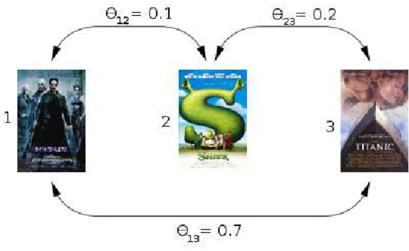
Structurally, this problem is an instance of MSDP. As previously mentioned, MSDP is a Facility Location Analysis, N P-hard problem. When pairwise scores θ satisfy the triangle inequality, MSDP admits a 2-approximation algorithm. The proof for this can be seen in Borodin et al. [2012] and Hassin et al. [1997]. On the other hand, it was demonstrated that if the triangle inequality is not satisfied, there is no polynomial time approximation algorithm to MSDP unless P = N P [Ravi et al., 1994]. The co-utility probabilities that we exploit in this work, namely pairwise scores θ, do not satisfy the triangle inequality, as illustrated in Figure 3.2. Hence none of the algorithms we analyse in this thesis have bounds on solution quality.

Figure 3.2. The triangle inequality is not satisfied, as θ13≥θ12+θ23.

(35)

3.3. Combining scores 19

(36)

(37)

Chapter 4 Algorithms and Validation

To tackle MSDP under a practical viewpoint, we studied two suboptimal, polynomial algorithms that are widely related to this problem. We also studied an integer program-ming approach toMSDP. These algorithms are the focus of Section 4.1. This problem cannot be solved efficiently by exact algorithms, albeit it is important to understand how it can be optimally solved. Besides addressing MSDP, we detail our baselines in Section 4.2. Finally, in Section 4.3, we present our validation schema for assessing the quality of our experimental results.

4.1 Algorithms to

MSDP

In this section, we address suboptimal and optimal algorithms to solve MSDP. Con-cerning the former category, we studied two popular heuristics with no bounds on solution quality. With respect to the latter, we describe how to model MSDP follow-ing the integer programmfollow-ing paradigm.

The algorithms addressed in this section are compatible with any recommender system where it is possible to estimate individual scores φ and pairwise scores θ to candidate items. Therefore, these algorithms area priori compatible with systems that employ both matrix factorization techniques and sketching/fingerprinting methods.

4.1.1 Heuristic

Greedy1

A widely used heuristic to MSDP is Greedy Best-First Search [Zuccon et al., 2012]. Henceforth, we will abbreviate it as Greedy1. In spite of not having solution quality bounds, it runs fast and yields acceptable solutions in practice. Greedy1 is shown in Algorithm 1. I is a set of items, Iφ corresponds to their individual scores, and Iθ

(38)

22 Chapter 4. Algorithms and Validation

corresponds to their pairwise scores. The output R is a set with N selected items, whereN ≤K.

Algorithm 1 Greedy1 Algorithm

Input: I ={i1, . . . , ik}, Iφ ={φi1, . . . , φik}, Iθ ={θi1i2, θi1i3, . . . , θik−1ik} , and N ≥1, |I| ≥N

Output: Selected items R 1: i⇐argmax

i∈I φi

2: R ⇐ {i}

3: I ⇐I \ {i}

4: while |R|< N do

5: j ⇐argmax j∈I

φj+ 1

|R|

X

k∈R θjk

6: R⇐R∪ {j} 7: I ⇐I\ {j}

8: end while

9: return R

Greedy1 starts by selecting the item that has the best individual score i. All otherN −1 selected items are chosen in a way that maximizes the equation in line 5, where the maximized set is comprised by all items R, that were already chosen, and the new item itself.

Greedy1 runs in polynomial time. The loop in line 4 will be executed exactly N −1 times. In line 5, an item is chosen out of K −1 in the worst case; in the best case, out of K −N + 1 ones. It means that O(K) items need to be analysed at each time. In line 5, the first part of the summation is performed inO(1) time; the second part, in O(|R|)time. An upper bound for the time complexity of Greedy1 is therefore O(N ×(K× |R|)) =O(KN2₎_{, given that}_|_R_{| ≤}_N_.

4.1.2 Heuristic

Greedy2

The second heuristic we studied, abbreviated as Greedy2, was proposed by Borodin et al. [2012]. It corresponds to Algorithm 2. Greedy2 is popular because, when pairwise scoresθ satisfy the triangle inequality, it is a 2-approximation algorithm toMSDP. It is almost the same as Greedy1, with a subtle yet relevant difference on line 5 – φj is multiplied by 1

2. This difference makes Greedy2 “non-oblivious”, as it is not selecting

the next element with respect to the originalMSDP objective function (Equation (3.7) on page 18).

(39)

4.1. Algorithms to MSDP 23

Algorithm 2 Greedy2 Algorithm

Input: I ={i1, . . . , ik}, Iφ = {φi1, . . . , φi_k}, Iθ = {θi1i2, θi1i3, . . . , θi_k−1ik}, and N ≥ 1, |I| ≥N

Output: Selected items R 1: i⇐argmax

i∈I φi

2: R ⇐ {i}

3: I ⇐I\ {i}

4: while |R|< N do

1 2φj+

1

|R|

X

k∈R θjk

6: R⇐R∪ {j}

7: I ⇐I\ {j} 8: end while

9: return R

maximize the objective function in line 3. In this loop,Greedy2 also updates setsI and R. An upper bound for the time complexity ofGreedy2 isO(N×(K×|R|)) = O(KN2₎_,

given that |R| ≤N.

4.1.3 Exact Solution

Since MSDP is N P-hard, it can only be solved efficiently by suboptimal algorithms. Despite that, it is important to understand how to model an exact algorithm toMSDP, especially if comparisons between optimal and suboptimal solutions are of interest. We decided to model MSDP under the integer programming paradigm because of the rather fast exact solvers available. It was also quite simple to map our objective function (Equation (3.7)) into an equivalent integer programming problem.

The parameters to model our integer programming problem are a set of items I ={i1, . . . , ik}, their corresponding individual scores Iφ={φi1, . . . , φik}, the pairwise

scores for all combinations of items in I, Iθ = {θi1i2, . . . , θik−1ik}, and the number of

items for selection N. We come up with binary variablesY ={y1, . . . , yk}to represent which items are selected (yj = 1 if and only if ij is selected), and rewriteMSDP as:

maximize 1

|I|

X

j∈I

yjφj+ 1

|I|2

X

j∈I X

k∈I|k6=j

yjykθjk,

subject to yi ∈ {0,1} ∀i, X

yi∈Y

yi =N.

(40)

MSDP’s products yjyk as variables xjk = yjyk ∀j,∀k. Considering that yj and yk are binary variables, we have the following constraints for variablesxjk:

xjk ≤yj

xjk ≤yk

xjk ≥yj+yk−1

That being stated, we rewrite our problem as:

maximize 1

|I|

X

j∈I

yjφj + 1

|I|2

X

j∈I X

k∈I|k6=j xjkθjk

subject to yi ∈ {0,1} ∀i xjk ≤yj

xjk ≤yk

xjk ≥yj +yk−1 X

yi∈Y

yi =N

4.2 Baselines

In this section, we describe the baselines with which we compare our method. Top−N adopts the Probability Ranking Principle (P RP) by selecting items according to their individual scores φ, generated by predictors such as PureSVD, exclusively. Mean-Variance Analysis, proposed by Wang [2009], andMaximal Marginal Relevance, widely exploited by works in diversity, break with the P RP by considering relations among candidate items for recommendation. Our method exploits co-utility probabilities un-der anMSDP framework and semantically differs from these baselines. To the best of our knowledge, there is no general-purpose, collaborative filtering selection techniques that model co-utilities in a way that is similar to ours. Despite that, comparisons among our method and these baselines are worthwhile, as we discuss in Chapter 5.

4.2.1 Top

−

N

Top−N is described in Algorithm 3. Input I corresponds to the set of K candidate items,Iφ is the related set of predicted individual scores, andN is the number of items for selection. OutputR is the set of selected items for recommendation.

(41)

4.2. Baselines 25

Algorithm 3 Top−N Algorithm

Input: I ={i1, . . . , ik},Iφ={φi1, . . . , φik}, and N ≥1,|I| ≥N

Output: Selected items R

1: R ⇐ {ij ∈I|φijis one of the N highest scores in Iφ}

2: return R

scores φ [Baeza-Yates and Ribeiro-Neto, 2011]. Alternatively, it is O(KlogK) if a complete ordering of items, according to their corresponding scores φ, is required.

4.2.2 Mean-Variance Analysis

Inspired by the Modern Portfolio Theory in finance, Wang [2009] proposes a method for ranking a list of items on the basis of its expected mean relevance and its variance. In that context, the variance works as a measure of risk. Based on this mean-variance principle, they devised a document ranking algorithm, abbreviated henceforth asMVA. MVAis shown in Algorithm 4. The inputI corresponds to the set ofK candidate items; Iφis the related set of individual scores, learned from a certain predictor;C is a covariance matrix estimated from users’ historic data; α is a real-valued risk regulator; N is the number of items for selection [Wang, 2009]. The outputRis the set of selected items for recommendation.

Algorithm 4 MVA Algorithm

Input: I = {i1, . . . , ik}, Iφ = {φi1, . . . , φik}, C = {c11, c12, . . . , ck−1k, ckk}, α, and

N ≥1, |I| ≥N

Output: Selected items R 1: R ⇐ ∅

2: while |R|< N do

φj −α×b2j −2α× X

k∈R

bkbjckj

4: R⇐R∪ {j}

5: I ⇐I\ {j} 6: end while

7: return R

The function in line 3 originally contains weights w for ranking regularization. We omitted these weights because we do not evaluate ranking aspects in this work – we focus on the selected set of items exclusively. Also in line 3, when α >0, the selection is risk-averse, while when α <0, it is risk-loving [Wang, 2009].

(42)

means that O(K) items need to be tested for selection at each time. For each test in line 3, the objective function is computed inO(|R|)time. An upper bound for the time complexity of MVA is thus O(N ×(K× |R|)) =O(KN2₎_{, given that} _|_R_{| ≤}_N_.

4.2.3 Maximal Marginal Relevance

Maximal Marginal Relevance (MMR) is a criterion that has been widely adopted in search and recommendation contexts as a means of diminishing redundancy while main-taining relevance [Carbonell and Goldstein, 1998; Vargas and Castells, 2011; Vieira et al., 2011; Zuccon et al., 2012]. MMR consists in a ranking formula that, as well as our method, takes the individual relevance of items and relations among them both into account. Given the wide scope of applications forMMR, there are different ways of implementing it. The implementation we use in this work is described in Zuccon et al. [2012] and is shown in Algorithm 5. Input I corresponds to the set of K candidate items; Iφ is the related set of individual scores, learnt from a certain predictor; ID is the set of pairwise dissimilarities computed for all items in I via users’ historic data; λ is a real-valued term regulator; and N is the number of items for selection. Output R is the set of selected items for recommendation.

Algorithm 5 MMR Algorithm

Input: I ={i1, . . . , ik}, Iφ = {φi1, . . . , φik}, ID = {Di1i2, . . . , Dik−1ik}, λ, and N ≥ 1, |I| ≥N

Output: Selected items R 1: R ⇐ ∅

2: while |R|< N do

λφj+ (1−λ)min k∈RDjk 4: R⇐R∪ {j}

5: I ⇐I\ {j}

6: end while

7: return R

In this work, we follow the choice of Zuccon et al. [2012] and use Kullback-Leibler Distance as the dissimilarity metric for pairs of items. Basically, this metric outputs how divergent the feedback that two items have received is. MMR is a polynomial time algorithm with an O(KN2₎_{upper bound for its time complexity. The derivation}

(43)

4.3. Validation Metrics 27

4.3 Validation Metrics

To validate our work, we use the explicit feedback users give over items as a utility metric: the better it is, the more useful the recommendations are [Breese et al., 1998]. For example, in movie ratings, where a 5-star movie is considered an excellent movie, we can assume that recommending a 5-star movie is more useful than recommend-ing a 4-star one [Ricci et al., 2011]. Furthermore, we consider that the utility of a recommendation system can be quantified by the utility of the recommendations it actually makes – rather than how close predictions are from the actual feedback given by users [Passos et al., 2011].

For all studied datasets, as we discuss in Chapter 5, feedback consists of ratings. Considering that we are focused on recommendations’ utility, and that we use ratings as a utility metric, we compare different algorithms by contrasting the ratings their selected items receive.

All the datasets we study consist of tuples(user, item, rating). We applied cross-validation in all experiments, and randomly partitioned the datasets into training and test data. Consequently, we ignored rating timestamps, whenever they were present, while splitting the data. Cross-validation is interesting in our case because we only analyse three datasets, and by crossing training and data partitions we increase the number of different scenarios on which we run experiments. Considering that rec-ommendation lists are generated over items in the test data, to which we know the actual ratings, our experiments simulate scenarios where users would rate all recom-mended items. Other works that opt for cross-validation are Vargas and Castells [2011] and Sarwar et al. [2001].

For each dataset, the training data is explored by predictors PureSVD and NNCosNgbr to generate individual scores φ. The training data is also used to esti-mate pairwise scores θ, as well as other pairwise information required by the baselines. For all tuples (user, item, rating) in the test data, we hide the corresponding rating: a ground-truth information that will be used as a metric of utility. The union of all (user, item)test pairs with a user in common corresponds to the set of candidate items for this user. This set, namely I, is one of the input parameters for all previously de-tailed algorithms. Individual scores are then predicted to all items in I, as well as pairwise scores for pairs of items in I.

We then run one of the studied algorithms and end up with a set of selected items R. At this point, we can retrieve the ground-truth rating for each selected item in R and analyse how useful the selection was in practice.

(44)

scope, diversity is defined as the opposite of similarity, and hence as a synonym for dissimilarity. Although not the focus of our work, we briefly investigate whether our method hurts recommendations’ diversity. The diversity metric we apply, intra-list distance (ILD), was proposed by Zhang and Hurley [2008] and works as follows:

ILD = 2

|R|(|R| −1) X

ik,il∈R,l<k

1−sim(ik, il), (4.1)

(45)

Chapter 5 Experimental Results

We examine different algorithms to MSDP, discussed in Chapter 4, by taking three different datasets into consideration: MovieLens 100K,1

MovieLens 1M,2

and Jester 1.3 For the MovieLens datasets, we considered that movies were liked by users – i.e., they were useful – if their ratings were equal or higher than 4;4

in the case of Jester 1, if they were equal or higher than 5.00. 5

The choice of these values is detailed in Section 5.1. For all experiments, PureSVD was executed with 50 latent factors, and the num-ber of neighbors in Dk₍_u_;_i₎ _{in Equation 3.1 was fixed in 60. After grid searches, these} two values yielded the bestTop −N results for both PureSVD and NNCosNgbr. Rec-ommendation lists have sizes N = 5,10,20 because they are popular values in the related literature. Considering that we use cross-validation, reported results are means of values per fold. Additionaly, we also compute means of ratings in some experiments. According to the Central Limit Theory, sampling distributions of means always follow the Gaussian distribution, so the distributions that we analyse, comprised by means, can be compared to each other via paired Student’s t-tests [Hastie et al., 2001].

This chapter is organized as follows. Section 5.1 brings a characterization of the datasets that we studied in this work. Section 5.2 compares different statistical estimators for pairwise scores θ. Section 5.3 contrasts different algorithms to MSDP and compares our method with different baselines in terms of utility. Section 5.4 examines how our method scales in time. Finally, Section 5.5 investigates the relation between our method and recommendations’ diversity.

1

http://www.grouplens.org/system/files/ml-100k.zip

2

http://www.grouplens.org/system/files/ml-1m.zip

3

http://goldberg.berkeley.edu/jester-data/jester-data-1.zip

4

Values range from 1 to 5. 5

Values range from -10.00 to 10.00.

(46)

30 Chapter 5. Experimental Results

5.1 Studied Datasets

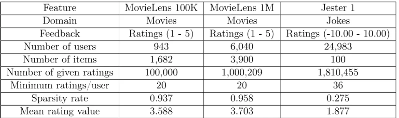
We performed experiments to validate our method over three different datasets: Movie-Lens 100K, MovieMovie-Lens 1M, and Jester 1. We chose to work with these datasets due to their popularity in the collaborative filtering literature. It is worth pointing out that the MovieLens datasets have some content and demographic data available. Nonethe-less, we did not exploit these data when learning recommendation models because our scope is limited to collaborative filtering. In this section we present a characterization of them in order to facilitate posterior experiment analyses. To start off, Table 5.1 summarizes some of the datasets’ main features.

Feature MovieLens 100K MovieLens 1M Jester 1

Domain Movies Movies Jokes

Feedback Ratings (1 - 5) Ratings (1 - 5) Ratings (-10.00 - 10.00)

Number of users 943 6,040 24,983

Number of items 1,682 3,900 100

Number of given ratings 100,000 1,000,209 1,810,455

Minimum ratings/user 20 20 36

Sparsity rate 0.937 0.958 0.275

Mean rating value 3.588 3.703 1.877

Table 5.1. Characterization of the studied datasets.

(47)

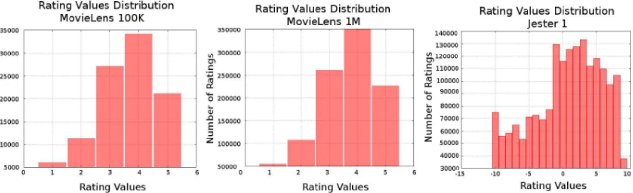
5.2. Comparing Estimators for Pairwise Scores 31

Figure 5.1. Distributions of ratings in the studied datasets. In the

graph that corresponds to Jester 1, each bar consists of ratings in intervals

[−10.00;−9.00),[−9.00;−8.00), . . . ,[9.00; 10.00].

can be approximated by a Gaussian distribution [Goldberg et al., 2001]. Considering these results, we henceforth assume that the hypothesis of Gaussian distributions is applicable for these ratings. Figure 5.1 also indicates that Jester 1 presents a higher rating variance, implying that rating values distant from the mean are more common in it than in the MovieLens datasets.

We adopted 4 as a threshold for high ratings, with respect to the MovieLens datasets, because this value is considered high by relevant works [Ricci et al., 2011; Jannach et al., 2011]. As for Jester 1, we decided to adopt 5.00 as a threshold because this value is significantly higher than the interval [2.00; 3.00), which is associated with most ratings in this dataset, and therefore seemed to be a safe choice. A more refined approach would consider that these thresholds vary from user to user. For example, users who tend to give lower ratings may find a 3-star movie useful. In spite of that, the generic thresholds that we adopted yielded useful recommendations to most users, as we discuss in this chapter. Consequently, we did not prioritize personalized thresholds.

5.2 Comparing Estimators for Pairwise Scores

In Chapter 3, we present two estimators for pairwise scores θ: Maximum Likelihood and Empirical Bayes.

(48)

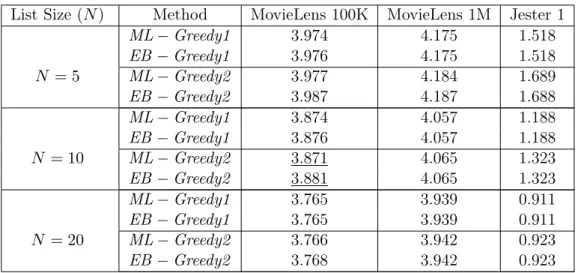
List Size (N) Method MovieLens 100K MovieLens 1M Jester 1

ML−Greedy1 3.974 4.175 1.518

EB−Greedy1 3.976 4.175 1.518

N = 5 ML−Greedy2 3.977 4.184 1.689

EB−Greedy2 3.987 4.187 1.688

ML−Greedy1 3.874 4.057 1.188

EB−Greedy1 3.876 4.057 1.188

N = 10 ML−Greedy2 3.871 4.065 1.323

EB−Greedy2 3.881 4.065 1.323

ML−Greedy1 3.765 3.939 0.911

EB−Greedy1 3.765 3.939 0.911

N = 20 ML−Greedy2 3.766 3.942 0.923

EB−Greedy2 3.768 3.942 0.923

Table 5.2. Mean ratings computed with different methods. ML−Greedy1

and ML−Greedy2 use Maximum Likelihood estimates for pairwise scores.

EB−Greedy1 and EB−Greedy2 use Empirical Bayes estimates instead. Re-ported results are averages of results obtained with 5-fold cross-validation.

Regarding Table 5.2, for each ML/EB pair of results with algorithm (Greedy1 or Greedy2), dataset, and N in common, we performed a paired t-test with a 95% confidence interval. Aside from the underlined result, all outcomes were statistically equivalent. This provides strong evidence that both estimators lead to very similar recommendations in terms of utility – i.e., mean rating given by users.

5.3 Comparing Algorithms to

MSDP

and Baselines

In this section, we investigate the effectiveness of different non-exact algorithms to MSDP. We also present a statistical comparison between non-exact and exact algo-rithms to MSDP. Finally, we compare our method with three different baselines.

5.3.1 Comparing Non-Exact Algorithms to

MSDP

To compareGreedy1 and Greedy2, two non-exact algorithms toMSDP, we computed individual scoresφ using PureSVD and NNCosNgbr as predictors, and pairwise scores θ were estimated with Empirical Bayes exclusively. Results are showed in Table 5.3, and statistical differences are underlined.

(49)

5.3. Comparing Algorithms to MSDP and Baselines 33

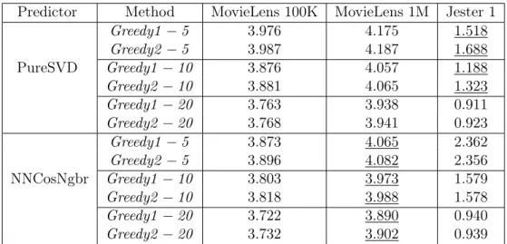
Predictor Method MovieLens 100K MovieLens 1M Jester 1

Greedy1−5 3.976 4.175 1.518

Greedy2−5 3.987 4.187 1.688

PureSVD Greedy1−10 3.876 4.057 1.188

Greedy2−10 3.881 4.065 1.323

Greedy1−20 3.763 3.938 0.911

Greedy2−20 3.768 3.941 0.923

Greedy1−5 3.873 4.065 2.362

Greedy2−5 3.896 4.082 2.356

NNCosNgbr Greedy1−10 3.803 3.973 1.579

Greedy2−10 3.818 3.988 1.578

Greedy1−20 3.722 3.890 0.940

Greedy2−20 3.732 3.902 0.939

Table 5.3. Mean ratings generated by solutions Greedy1 and Greedy2 for rec-ommendation lists with sizesN = 5,10,20. Greedy1−5corresponds to solutions with sizeN = 5generated byGreedy1, for example. Reported results are averages of results obtained with 5-fold cross-validation.

Greedy2 generated statistically different results, Greedy2 was responsible for the best values. For the Jester 1 dataset, whose ratings range from -10.00 to 10.00, the gains were up to 11% with Greedy2 −5 outperforming Greedy1 −5. As for the MovieLens datasets, whose ratings range from 1 to 5, the gains were up to 0.4% for MovieLens 1M, with Greedy2 −5 winning over Greedy1 −5.

It is important to notice that the best mean ratings for the MovieLens datasets were generated with predictor PureSVD. As for the Jester 1 dataset, NNCosNgbr yielded better results. In the latter case, it is likely that NNCosNgbr has benefited from Jester 1’s low sparsity, as it is a memory-based predictor sensitive to high sparsity scenarios. Finally, it is clear in Table 5.3 that Greedy1/Greedy2 differences tend to get smaller as N grows. This is a consequence of the fact that, with larger N values, the difference between N and the number of items available for selection becomes smaller, thus allowing higher overlaps between solution.

5.3.2 Comparing Non-Exact and Exact Algorithms to

MSDP

(50)

not use both predictors because comparing their performances is not the goal of this experiment and generating exact solutions to MSDP is very time-consuming. For the same reason, we relied exclusively on predictor NNCosNgbr for the Jester 1 dataset. After the variables, parameters, and restrictions ofExact were defined, we passed them to IBM’s CPLEX optimizer [ILOG, Inc, 2013].

To contrast Greedy2 and Exact, we divided the dataset MovieLens 100K into 5 folds with approximately the same size randomly. As for MovieLens 1M and Jester 1, the number of folds was 10, as generating exact solutions to a test set is an exponential time task and takes many hours to be completed. In all cases, one of the folds was chosen for test and the others were used for training. We did not perform cross-validation either due to time constraints.

To make it possible to compute the exact solutions and perform comparisons that could make sense in practical scenarios, we adopted a timeout of 20 seconds. We dis-carded all exact solutions that would take more than that, and only compared optimal solutions obtained below this time threshold with their corresponding suboptimal ones. Solutions that take more than 20 seconds to compute may share specific characteristics that could change our analysis, but at least they corresponded to less than 15% of all cases. The mean ratings obtained by different solutions are listed in Table 5.4.

Method MovieLens 100K MovieLens 1M Jester 1

Greedy2 −5 3.971 4.166 2.136

Exact−5 4.003 4.184 2.149

Greedy2 −10 3.900 4.137 1.369

Exact−10 3.907 4.148 1.370

Greedy2 −20 3.770 3.947 1.075

Exact−20 3.771 3.951 1.078

Table 5.4. Mean ratings computed withGreedy2 andExact for recommendation

lists with sizesN = 5,10,20. Greedy2−5corresponds to solutions with sizeN = 5

generated by Greedy2, for example.

We performed a paired t-test with a 95% confidence interval and all mean ratings obtained withGreedy2 were statistically equivalent to the corresponding ones prompted byExact. These results draw attention to the idea that, in practice,Greedy2 is a good approach to MSDP.

A case whereGreedy2 and Exact lead to different solutions works as follows. Let us consider a set of candidate items I = {i1, i2, i3} with corresponding sets of scores

Iφ ={φi1 = 0.9, φi2 = 0.85, φi3 = 0.85} and Iθ ={θi1i2 = 0.7, θi1i3 = 0.6, θi2i3 = 0.9}. If

(51)

will select i1 and i2. The greedy choice of starting the selection by choosing the item

with the highest score φ not necessarily leads to the optimal solution, as the example illustrates. This situation happens in practice, but Table 5.4 indicates that, regardless of it, selections prompted by both Exact and Greedy2 are likely to be similarly useful.

5.3.3 Comparing Our Method to Baselines

We decided to compareGreedy2 withTop−N,MVA, andMMRin order to understand some of its different aspects. With respect to Top −N, we wanted to evaluate how the exploitation of co-utility alone can improve recommendations. As for MVA and MMR, we were interested in contrasting Greedy2 with methods that also abandon the assumption that items are independent. MMR, in particular, also maps into MSDP, although the semantics of its pairwise scores is related to diversity – not to co-utility.

For all methods, individual scores were predicted by PureSVD and NNCosNgbr. Greedy2’s pairwise scores were calculated with the Empirical Bayes estimator. We set MVA’s parameter α = 0.05 after a grid search involving values that ranged from -5.0 to 5.0, i.e., MVA is slightly risk-lover in our experiments. The parameter α = 0.05 prompted the best MVA’s results. As to MVA’s covariance matrix, we computed it by considering, for every pair of items, the ratings they received by a common set of users. With respect to MMR, we followed Zuccon et al. [2012] and adopted Kullback-Leibler distance for computing the dissimilarity between items’ rating distributions. There are several ways of measuring items’ dissimilarity, and even though this im-plementation of MMR uses differences in rating distributions as a proxy for diversity, many methods for measuring diversity are based on item content [Ricci et al., 2011]. The use of rating distributions is particularly indispensable when a strict collaborative filtering schema has to be adopted, or when no information about the items is available. One of the reasons why we chose this implementation of MMR is because it does not use content information to devise pairwise scores, so the comparison becomes fairer.

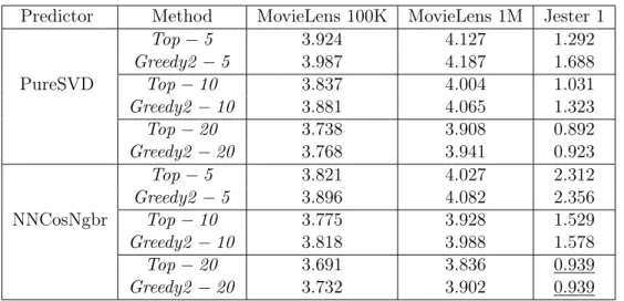
Results that contrast Greedy2 and Top −N are listed in Table 5.5, Table 5.6 and Figure 5.2. As for MVA and MMR, they are compared with Greedy2 in Ta-ble 5.7, TaTa-ble 5.8, Figure 5.3, and Figure 5.4. For all experiments reported in taTa-bles, we performed a paired t-test with a 95% confidence interval. Underlined results are statistically equivalent.

(52)

Top−5 3.924 4.127 1.292

Greedy2 −5 3.987 4.187 1.688

PureSVD Top−10 3.837 4.004 1.031

Greedy2−10 3.881 4.065 1.323

Top−20 3.738 3.908 0.892

Greedy2−20 3.768 3.941 0.923

Top−5 3.821 4.027 2.312

Greedy2 −5 3.896 4.082 2.356

NNCosNgbr Top−10 3.775 3.928 1.529

Greedy2−10 3.818 3.988 1.578

Top−20 3.691 3.836 0.939

Greedy2−20 3.732 3.902 0.939

Table 5.5. Mean ratings computed with Top−N and Greedy2 for

recommen-dation lists with sizes N = 5,10,20. Greedy2−5 corresponds to solutions with size N = 5generated by Greedy2, for example. Reported results are averages of results obtained with 5-fold cross-validation.

with Greedy2 −5 outperforming Top−5. As for the MovieLens datasets, they were up to 2% withGreedy2 −5 outperformingTop−5 for MovieLens 100K. Although the difference between Greedy2 and Top −N in Table 5.5 may seem small on average, it has an impact on recommender systems [Bell and Koren, 2007].

In absolute terms for Jester 1,Greedy2 outperformsTop−N by 0.396 points in the best case (Greedy2 −5 andTop−5) and by 0.000 in the worst case (Greedy2 −20 and Top−20). With respect to the MovieLens datasets, Greedy2 wins over Top−N by 0.228 points in the best case (Greedy2 −10 and Top−10 for MovieLens 1M) and by 0.030 in the worst case (Greedy2 −20 and Top −20 for MovieLens 100K).

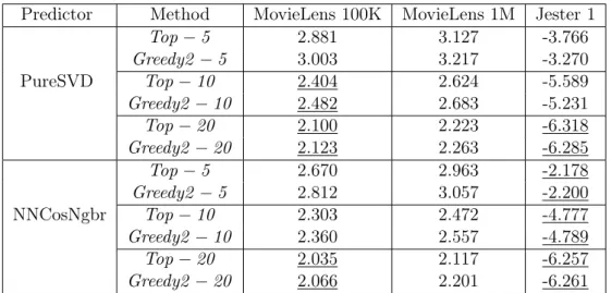
Some works suggest that it is worse to recommend an item the user dislikes than to not recommend an item she likes [Hansen and Golbeck, 2009; Ricci et al., 2011]. In order to give continuity to our analysis, we exploit this idea by assuming that low ratings are given to disliked items and compare the lowest ratings obtained with Top−N andGreedy2. Instead of focusing on all recommended items, this experiment concerns only the worst rated item in each recommendation. Results are arranged in Table 5.6. Underlined values are statistically equivalent.

(53)

Top−5 2.881 3.127 -3.766

Greedy2−5 3.003 3.217 -3.270 PureSVD Top−10 2.404 2.624 -5.589

Greedy2−10 2.482 2.683 -5.231

Top−20 2.100 2.223 -6.318

Greedy2−20 2.123 2.263 -6.285

Top−5 2.670 2.963 -2.178

Greedy2−5 2.812 3.057 -2.200 NNCosNgbr Top−10 2.303 2.472 -4.777

Greedy2−10 2.360 2.557 -4.789

Top−20 2.035 2.117 -6.257

Greedy2−20 2.066 2.201 -6.261

Table 5.6. Lowest ratings generated byTop−N and Greedy2 for

recommenda-tion lists with sizesN = 5,10,20. Reported values are averages of results obtained with 5-fold cross-validation.

and Top−5 for MovieLens 100K) and by 0.023 in the worst case (Greedy2 −20 and Top −20 for MovieLens 100K). Finally, recommendations generated for Jester 1 with NNCosNgbr were particularly similar for both Greedy2 and Top −N, with equivalent mean ratings for all N values.

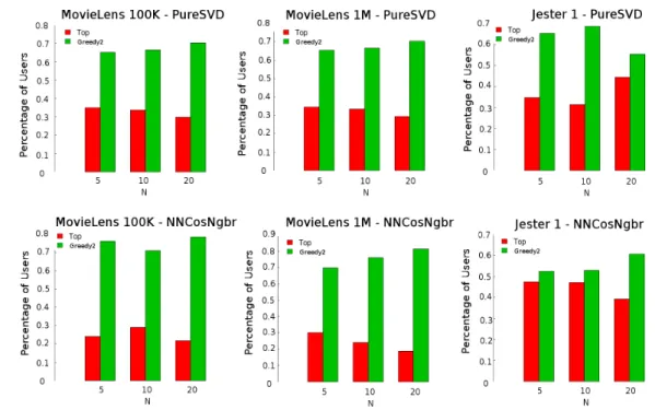
Thus far, we have based our analysis on averages of ratings. Albeit useful, av-erages are not statistically robust measures [Zaki and Meira, 2014]. Hence, to have a better idea of the difference between Greedy2 and Top−N, we extend our analysis to a percentual approach. Specifically, we computed how many times each method yielded the highest ratings and reported percentages in Figure 5.2.

Figure 5.2 leads to a succint Win/Loss analysis. Greedy2 generates the highest mean ratings to approximately 65% of users. The percentages associated withGreedy2 tend to increase asN grows, which suggests that our method brings gain to more users when more recommendations are generated. We also investigated whether our method works best to users with small historical data, or to users who tend to give particularly high/low ratings, but no patterns were noticed.

(54)

Figure 5.2. Percentages of users to which Top−N andGreedy2 have won over each other, in terms of highest mean rating given to generated recommendations.

gains were up to 3% for the MovieLens datasets, with Greedy2 −5 outperforming MMR−5 for MovieLens 100K.

In absolute terms for Jester 1,Greedy2 surpassesMVAby 1.210 points in the best case (Greedy2 −5 versusMVA−5) and by 0.059 in the worst case (Greedy2 −20 ver-susMVA−20). As for the MovieLens datasets, Greedy2 outperforms MVA by 0.235 points in the best case (Greedy2 −10 versus MVA−10 for MovieLens 1M) and by 0.040 in the worst case (Greedy2 −20 versusMVA−20 for MovieLens 1M). With re-spect toMMR for Jester 1,Greedy2 wins over it by 0.396 points at most (Greedy2 −5 versus MMR−5) and by 0.000 at least (Greedy2 −20 versus MMR−20). Greedy2 outperforms MMR for the MovieLens datasets by 0.103 points in the best case (Greedy2 −5 versus MMR−5 for MovieLens 100K) and by 0.041 in the worst case (Greedy2 −20 versus MMR−20 for MovieLens 1M).

We repeated the analysis of lowest scores and percentages, performed forTop−N and Greedy2, over MVA, MMR, and Greedy2. Results are summarized in Table 5.8, Figure 5.3, and Figure 5.4. Underlined values are statistically equivalent, according to a paired t-test with a 95% confidence interval.

(55)

MVA−5 3.923 4.128 1.092

MMR−5 3.884 4.120 1.292

Greedy2−5 3.987 4.187 1.688

PureSVD MVA−10 3.830 4.013 0.950

MMR−10 3.799 4.012 1.031

Greedy2−10 3.881 4.065 1.323

MVA−20 3.720 3.901 0.864

MMR−20 3.698 3.900 0.892

Greedy2−20 3.768 3.941 0.923

MVA−5 3.833 4.027 1.146

MMR−5 3.801 4.022 2.312

Greedy2−5 3.896 4.082 2.356

NNCosNgbr MVA−10 3.768 3.927 1.338

MMR−10 3.760 3.926 1.559

Greedy2−10 3.818 3.988 1.578

MVA−20 3.677 3.824 0.859

MMR−20 3.677 3.832 0.939

Greedy2−20 3.732 3.902 0.939

Table 5.7. Mean ratings computed with MVA,MMR, and Greedy2 for

recom-mendation lists with sizes N = 5,10,20. Greedy2−5 corresponds to solutions with sizeN = 5generated byGreedy2, for example. Reported results are averages of results obtained with 5-fold cross-validation.

Once again, values obtained with MMR were somewhat similar to those prompted by Top −N. MVA performed better thanMMR with respect to the MovieLens datasets and the opposite was noticed with respect to Jester 1. In all cases, Greedy2 led to superior or statistically equivalent lowest ratings, when compared with both baselines. In terms of ratings for Jester 1, Greedy2 exceeds MVA by 2.087 points in the best case (Greedy2 −5 and MVA−5) and by 0.064 in the worst case (Greedy2 −20 and MVA−20). As for the MovieLens datasets, Greedy2 outperforms MVA by 0.133 points at most (Greedy2 −5 and MVA−5 for MovieLens 100K) and by 0.048 in the worst case (Greedy2 −20 andMVA−20 for MovieLens 100K). With respect toMMR for Jester 1, Greedy2 surpassed it by 0.495 points in the best case (Greedy2 −5 and MMR−5) and was surpassed by it by 0.012 points in the worst case (Greedy2 −10 and MMR−10). Regarding the MovieLens datasets, Greedy2 outperformed MMR by 0.205 points at most (Greedy2 −5 and MMR−5 for MovieLens 100K) and by 0.054 points at least (Greedy2 −20 and MMR−20 for MovieLens 100K).

Exploiting item co-utility to improve recommendations

EXPLOITING ITEM CO-UTILITY

ALINE BESSA

EXPLOITING ITEM CO-UTILITY

TO IMPROVE RECOMMENDATIONS

Advisor: Nivio Ziviani

Co-Advisor: Adriano Veloso

Belo Horizonte

Acknowledgments

Abstract

Contents

Chapter 1

Introduction

1.1

Work Contributions

1.2

Research Development

1.3

Work Outline

Chapter 2

Related Work

2.1

Predictors for

Top

−

N

Recommendations

2.2

Exploiting Relations among Items

2.3

Max-Sum Dispersion Problem (MSDP

)

Chapter 3

Basic Concepts

3.1

Individual Scores

3.1.1

NNCosNgbr

3.1.2

PureSVD

3.2

Pairwise Scores

3.3

Combining scores

Chapter 4

Algorithms and Validation

4.1

Algorithms to

MSDP

4.1.1

Heuristic

Greedy1

4.1.2

Heuristic

Greedy2

4.1.3

Exact Solution

4.2

Baselines

4.2.1

Top

−

N

4.2.2

Mean-Variance Analysis

4.2.3

Maximal Marginal Relevance

4.3

Validation Metrics

Chapter 5

Experimental Results

5.1

Studied Datasets

5.2

Comparing Estimators for Pairwise Scores

5.3

Comparing Algorithms to

MSDP

and Baselines

5.3.1