Quantifying contributions to the recent temperature variability in the tropical tropopause layer

(1)

www.atmos-chem-phys.net/15/5815/2015/ doi:10.5194/acp-15-5815-2015

Quantifying contributions to the recent temperature variability in

the tropical tropopause layer

W. Wang1,2, K. Matthes2,3, and T. Schmidt4

1_{Freie Universität Berlin, Institut für Meteorologie, Berlin, Germany} 2_{GEOMAR Helmholtz-Zentrum für Ozeanforschung Kiel, Kiel, Germany} 3_{Christian-Albrechts Universität zu Kiel, Kiel, Germany}

4_{Helmholtz Zentrum Potsdam, Deutsches GeoForschungsZentrum (GFZ), Potsdam, Germany}

Correspondence to:W. Wang (wuke.wang@fu-berlin.de)

Received: 1 August 2014 – Published in Atmos. Chem. Phys. Discuss.: 28 August 2014 Revised: 22 April 2015 – Accepted: 8 May 2015 – Published: 26 May 2015

Abstract. The recently observed variability in the tropi-cal tropopause layer (TTL), which features a warming of 0.9 K over the past decade (2001–2011), is investigated with a number of sensitivity experiments from simulations with NCAR’s CESM-WACCM chemistry–climate model. The ex-periments have been designed to specifically quantify the contributions from natural as well as anthropogenic factors, such as solar variability (Solar), sea surface temperatures (SSTs), the quasi-biennial oscillation (QBO), stratospheric aerosols (Aerosol), greenhouse gases (GHGs) and the de-pendence on the vertical resolution in the model. The re-sults show that, in the TTL from 2001 through 2011, a cooling in tropical SSTs leads to a weakening of tropical upwelling around the tropical tropopause and hence rela-tive downwelling and adiabatic warming of 0.3 K decade−1_;

stronger QBO westerlies result in a 0.2 K decade−1

warm-ing; increasing aerosols in the lower stratosphere lead to a 0.2 K decade−1 _{warming; a prolonged solar minimum}

con-tributes about 0.2 K decade−1

to a cooling; and increased GHGs have no significant influence. Considering all the fac-tors mentioned above, we compute a net 0.5 K decade−1

warming, which is less than the observed 0.9 K decade−1 warming over the past decade in the TTL. Two simulations with different vertical resolution show that, with higher verti-cal resolution, an extra 0.8 K decade−1_{warming can be}

simu-lated through the last decade compared with results from the “standard” low vertical resolution simulation. Model results indicate that the recent warming in the TTL is partly caused by stratospheric aerosols and mainly due to internal variabil-ity, i.e. the QBO and tropical SSTs. The vertical resolution

can also strongly influence the TTL temperature response in addition to variability in the QBO and SSTs.

1 Introduction

(2)

forc-ings of the climate system and hence is a useful indicator for climate change (Fueglistaler et al., 2009).

Over the past decade, a remarkable warming has been cap-tured by Global Positioning System Radio Occultation (GPS-RO) data in the TTL region (Schmidt et al., 2010; Wang et al., 2013). This might indicate a climate change signal, with pos-sible important impacts on stratospheric climate: e.g. tropi-cal tropopause temperatures dominate the amount of water vapour entering the stratosphere (Dessler et al., 2013, 2014; Solomon et al., 2010; Gettelman et al., 2009; Randel and Jensen, 2013). So far a long-term cooling in the lower strato-sphere has been reported from the 1970s to 2000, although there are large differences between different data sets (Ran-del et al., 2009; Wang et al., 2012; Fueglistaler et al., 2013). The exact reason for the recent warming is therefore of great interest. An interesting issue is also whether this warming will continue or change in sign in the future and how well climate models can reproduce such a strong warming over 1 decade or longer time periods.

Based on model simulations, Wang et al. (2013) suggested that the warming around the tropical tropopause could be a result of a weaker tropical upwelling, which implies a weakening of the Brewer–Dobson circulation (BDC). How-ever, the strengthening or weakening of the BDC is still under debate (Butchart, 2014, and references therein). Results from observations indicate that the BDC may have slightly decel-erated (Engel et al., 2009; Stiller et al., 2012), while estimates from a number of chemistry–climate models (CCMs) show in contrast a strengthening of the BDC (Butchart et al., 2010; Li et al., 2008; Butchart, 2014). The reason for the discrep-ancy between observed and modelled BDC changes, as well as the mechanisms of the BDC response to climate change, is still under discussion (Oberländer et al., 2013; Shepherd and McLandress, 2011). The trends in the BDC may be dif-ferent in difdif-ferent branches of the BDC (Lin and Fu, 2013; Oberländer et al., 2013). Bunzel and Schmidt (2013) show that the model configuration, i.e. the vertical resolution and the vertical extent of the model, can also impact trends in the BDC.

There are a number of other natural and anthropogenic fac-tors besides the BDC which influence radiative, chemical and dynamical processes in the TTL. One prominent candidate for natural variability is the sun, which provides the energy source of the climate system. The 11-year solar cycle is the most prominent natural variation on the decadal timescale (Gray et al., 2010). Solar variability influences the tempera-ture directly through radiative effects and indirectly through radiative effects on ozone and dynamical effects. The maxi-mum response in temperature occurs in the equatorial upper stratosphere during solar maximum conditions, and a distinct secondary temperature maximum can be found in the equa-torial lower stratosphere around 100 hPa (SPARC-CCMVal, 2010; Gray et al., 2010).

Sea surface temperatures (SSTs) also influence the TTL by affecting the dynamical conditions and subsequently the

propagation of atmospheric waves and hence the circulation. Increasing tropical SSTs can enhance the BDC, which in turn cools the tropical lower stratosphere through enhanced up-welling (Grise and Thompson, 2012, 2013; Oberländer et al., 2013). The quasi-biennial oscillation (QBO) is the dominant mode of variability throughout the equatorial stratosphere and has important impacts on the temperature structure as well as the distribution of chemical constituents like wa-ter vapour, methane and ozone (Baldwin et al., 2001). Be-side the switch between easterlies and westerlies with a pe-riod of about 28 months, the QBO undergoes some cycle-to-cycle variability, e.g. variations in period and amplitude and shifts to westerlies or easterlies, which may influence the long-term variability in the TTL (Kawatani and Hamilton, 2013). Stratospheric aerosols absorb outgoing long-wave ra-diation and lead to additional heating in the lower strato-sphere, which maximizes around 20 km (Solomon et al., 2011; SPARC-CCMVal, 2010, chapter 8).

While greenhouse gases (GHGs) warm the troposphere, they cool the stratosphere at the same time by releasing more radiation into space. Warming of the troposphere and cooling of the stratosphere affect the temperature in the TTL directly, as well as indirectly, by changing chemical trace gas distri-butions and wave activities (SPARC-CCMVal, 2010).

In climate models, a sufficient high vertical resolution is important in order for models to correctly represent dynami-cal processes, such as wave propagation into the stratosphere and wave–mean flow interactions. High vertical resolution is also important to generate a self-consistent QBO (Richter et al., 2014). Meanwhile, vertical resolution is essential for a proper representation of the thermal structure in the model: e.g. models with coarse vertical resolution can not simulate the tropopause inversion layer (a narrow band of temper-ature inversion above the tropopause associated with a re-gion of enhanced static stability) well (Wang et al., 2013; SPARC-CCMVal, 2010, chapter 7). Coarse vertical resolu-tion is also still a problem for analysing the effects of El-Niño Southern Oscillation (ENSO) and the QBO onto the tropical tropopause (Zhou et al., 2001; SPARC-CCMVal, 2010, chap-ter 7).

In this study we use a series of simulations with NCAR’s Community Earth System Model (CESM) model (Marsh et al., 2013) to quantify the contributions of the above dis-cussed factors – Solar, SSTs, QBO, Aerosol and GHGs – to the recently observed variability in the TTL.

(3)

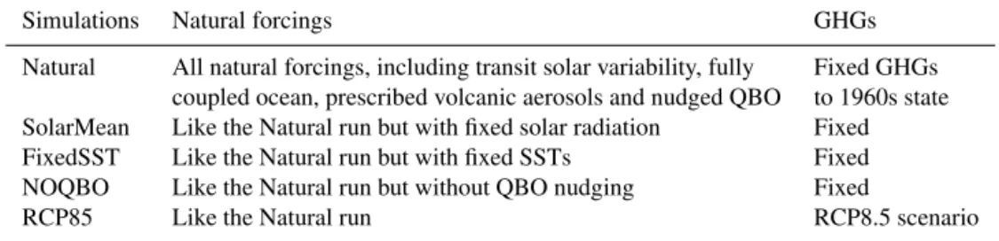
Table 1.Overview of fully coupled CESM-WACCM simulations (1955–2099).

Simulations Natural forcings GHGs

Natural All natural forcings, including transit solar variability, fully Fixed GHGs

coupled ocean, prescribed volcanic aerosols and nudged QBO to 1960s state

SolarMean Like the Natural run but with fixed solar radiation Fixed

FixedSST Like the Natural run but with fixed SSTs Fixed

NOQBO Like the Natural run but without QBO nudging Fixed

RCP85 Like the Natural run RCP8.5 scenario

2 Model simulations and method description 2.1 Fully coupled CESM-WACCM simulations

The model used here is NCAR’s CESM version 1.0. CESM is a fully coupled model system, including an interactive ocean (POP2), land (CLM4), sea ice (CICE) and atmosphere (CAM/WACCM) component (Marsh et al., 2013). As the at-mospheric component we use the Whole Atmosphere Com-munity Climate Model (WACCM), version 4. WACCM4 is a CCM with detailed middle atmospheric chemistry and a fi-nite volume dynamical core, extending from the surface to about 140 km (Marsh et al., 2013). The standard version has 66 (W_L66) vertical levels, which means about 1 km verti-cal resolution in the TTL and in the lower stratosphere. All simulations use a horizontal resolution of 1.9◦_×

2.5◦

(lati-tude×_{longitude) for the atmosphere and approximately 1}◦ for the ocean.

Table 1 gives an overview of all coupled CESM simula-tions. A control run was performed from 1955 to 2099 (Natu-ral run hereafter) with all natu(Natu-ral forcing including spect(Natu-rally resolved solar variability (Lean et al., 2005), a fully coupled ocean, volcanic aerosols following the SPARC (Stratospheric Processes and their Role in Climate) CCMVal (Chemistry– Climate Model Validation) REF-B2 scenario recommenda-tions (see details in SPARC-CCMVal, 2010) and a nudged QBO. The QBO is nudged by relaxing the modelled tropi-cal zonal winds to observations between 22◦

S and N, using a Gaussian weighting function with a half width of 10◦

de-caying latitudinally from the equator. Full vertical relaxation extends from 86 to 4 hPa, which is half the strength of the level below and above this range and 0 for all other levels (see details in Matthes et al., 2010; Hansen et al., 2013). The QBO forcing time series in CESM is determined from the observed climatology of 1953–2004 via filtered spectral de-composition of that climatology. This gives a set of Fourier coefficients that can be expanded for any day and year in the past and the future. Anthropogenic forcings like GHGs and ozone-depleting substances (ODSs) are set to constant 1960s conditions. Using the Natural run as a reference, a series of four sensitivity experiments were performed by system-atically switching on or off several factors. The SolarMean run uses constant solar cycle values averaged over the past four observed solar cycles. The FixedSST run uses monthly

varying climatological SSTs calculated from the Natural run and therefore neglects variability from varying SSTs such as ENSO. In the NOQBO run the QBO nudging has been switched off which means weak zonal mean easterly winds develop in the tropical stratosphere. An additional simula-tion, RCP85, uses the same forcings as the Natural run but in addition includes increases in anthropogenic GHGs and ODSs forcings. These forcings are based on observations from 1955 to 2005, after which they follow the representa-tive concentration pathways (RCPs) RCP8.5 scenario (Mein-shausen et al., 2011).

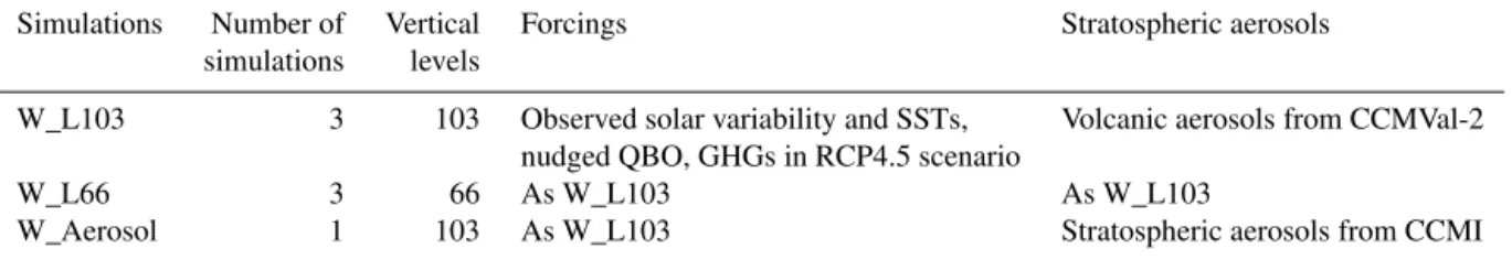
2.2 WACCM atmospheric stand-alone simulations Instead of using the fully coupled CESM-WACCM version, WACCM can be integrated in an atmospheric stand-alone configuration with prescribed SSTs and sea ice. Beside the standard version with 66 vertical levels (W_L66), we have also performed simulations with a finer vertical resolution, with 103 vertical levels and about 300 m vertical resolution in the TTL and lower stratosphere (W_L103) (Gettelman and Birner, 2007; Wang et al., 2013).

(4)

Table 2.Overview of WACCM atmospheric stand-alone simulations (2001–2010).

Simulations Number of Vertical Forcings Stratospheric aerosols

simulations levels

W_L103 3 103 Observed solar variability and SSTs, Volcanic aerosols from CCMVal-2

nudged QBO, GHGs in RCP4.5 scenario

W_L66 3 66 As W_L103 As W_L103

W_Aerosol 1 103 As W_L103 Stratospheric aerosols from CCMI

2.3 Estimation of factor contributions

For a pair of reference and single-factor runs (e.g. Natural and SolarMean), all configuration and drivers are the same except for the long-term variability of the respective factor (e.g. Solar). Temperature differences Tdiff(x, t )between the

reference and single-factor runs (e.g. Natural – SolarMean) can be estimated by a linear regression:

Test(x, t )=c(x)X(t ), (1)

whereTest(x, t )is an estimate ofTdiff(x, t )at each grid point

(x) and each simulation time (t).X(t )is the time series of the respective factor (e.g. Solar) andc(x)are the coefficients of that factor at each grid point.

Then the contributions of that factor to the recent warming in the TTL can be estimated as

Tfac(x)=c(x)bfac, (2)

whereTfac(x)represents the factor contribution to the recent

temperature trend,c(x)are the coefficients andbfacis the

ob-served linear trend of that factor during 2001–2011 (Fig. 1). The standard error (SE) can be used to estimate the un-certainty of the regressed coefficientsc(x), which is defined by

(SE)2=

Pn t=1e2t

(neff−2)Pn_t=1(Xt−X)2

, (3)

where n is the sample size, e=Tdiff−Test are the

residu-als andX is the mean value.neff is the effective number of

degrees of freedom, with consideration of the effect of auto-correlation, which is determined by

neff=n

1−ra

1+ra

, (4)

where ra is the lag-1 autocorrelation coefficient (Wigley,

2006).

For the estimated coefficientsc, the test statistics

t_test= c

SE (5)

has the Student’st distribution withneff−2 degrees of

free-dom.

Beside the regressions described above, the Pearson’s cor-relations (r) between temperature differences (Tdiff) and the

respective factor (X) were also estimated. The test statistics

t_test=r

r

neff−2

1−r2 (6)

has the Student’st distribution withneff−2 degrees of

free-dom, and the effective number of degrees of freedom can be estimated by

1

neff

=1

n+

2

nra1ra2, (7)

wherera1,ra2are the lag-1 autocorrelation coefficients of the

two time series in calculating the Pearson’s correlation re-spectively.

Such regressions, correlations and 11-year trend estima-tions were applied to all factors, i.e. Solar, SSTs, QBO, GHGs and stratospheric aerosols.

Special attention is given to the region 20◦_S–20◦_N

lat-itude and 16–21 km height, which is mainly the observed warming area in the TTL (see below). Hereafter, we use the average trend over this area to discuss the exact contribution of every factor to the temperature trend in the TTL.

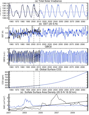
2.4 Forcings in observations and model simulations Figure 1 shows the time series of both natural and anthro-pogenic forcings over past and future decades in observations (black) and model experiments (blue). Observed linear trends during 2001–2011 are highlighted with straight lines.

Observations of the solar variability show that the total so-lar irradiance (TSI) exhibits a clear 11-year soso-lar cycle varia-tion of about 1 W m−2_{between sunspot minimum (}_S

min) and

sunspot maximum (Smax) in the past (Gray et al., 2010). The

future projection in the Natural run is a repetition of the last four observed solar cycles (Fig. 1a, blue line). With a de-layed and smaller amplitude return to maximum conditions, the observed TSI significantly (over 95 %) decreased during 2001–2011 (Fig. 1a, straight black line).

Figure 1b shows the variability of tropical (20◦

S–20◦

(5)

ex-(a) Total Solar Irradiance

1960 1970 1980 1990 2000 2010 2020 2030 2040 2050 2060 2070 2080 2090 1360.8

1361.0 1361.2 1361.4 1361.6 1361.8 1362.0

TSI (W/m

2)

(b) SST (20 S-N)

1960 1970 1980 1990 2000 2010 2020 2030 2040 2050 2060 2070 2080 2090 -0.5

0.0 0.5

SST (K)

QBO2

1960 1970 1980 1990 2000 2010 2020 2030 2040 2050 2060 2070 2080 2090 -2

-1 0 1 2

QBO2 (s.d.)

(d) Global Surface CO2

1960 1970 1980 1990 2000 2010 2020 2030 2040 2050 2060 2070 2080 2090 300

400 500 600 700 800 900

CO2 (ppm)

(e) Sulfate Surface Area Density (20 S-N 18-32 km)

2001 2003 2005 2007 2009 -1

0 1 2

SAD (um

2/cm 3)

Figure 1.Time series of forcing data sets used for the simulations

from 1955 through 2099.(a)TSI from observations (black), Natural

(solid blue) and SolarMean (dashed blue) runs.(b)SST anomalies

from HadISSTs (black), Natural (solid blue) and FixedSST (dashed

blue) runs.(c)QBO2 (see text for details) from observations (black)

and Natural (solid blue) run.(d)Global surface CO2concentration

from observations (black, overlapped with the blue line), RCP85

(solid blue) and Natural (dashed blue) runs.(e)AOD (532 nm, 18–

32 km) from the CCMI (black) and the CCMVal2 (blue) projects for the time 2001–2010. The black solid straight lines in each subfigure are the linear fits of the respective forcing during 2001–2011.

periment (blue line). Both the observed and simulated tropi-cal SSTs show a statistitropi-cally significant (over 95 %) decrease from 2001 to 2011. Note that there is a strong drop in SSTs around 1992 in the model, which does not occur in observa-tions. This might be caused by an overestimated response to the Pinatubo eruption in the CESM-WACCM model (Marsh et al., 2013; Meehl et al., 2012).

The QBO variations are represented by a pair of or-thogonal time series QBO1 and QBO2, which are con-structed from the equatorial zonal winds over 70–10 hPa (Randel et al., 2009). The observed QBO2 (data from the FU Berlin: http://www.geo.fu-berlin.de/en/met/ag/strat/ produkte/qbo/index.html), which is the dominate mode of QBO in the tropical lower stratosphere, shows an increase (a shift towards westerlies or stronger westerlies) during 2001– 2011 (Fig. 1c, straight black line). Note that this short-term linear trend of the QBO2 is sensitive to the start and

end-ing years. However, a further analysis for 2001–2012 endend-ing with a relative minimum of QBO2 confirms this significant increase of QBO2 (not shown).

As shown in Fig. 1d, GHGs show a steady increase after 2001. The increasing rate of global CO2release from 2001

to 2011 is close to the RCP8.5 scenario.

Similar to the GHGs, observed stratospheric aerosols (aerosol optical depth, AOD) have been steadily increasing since 2001 (Solomon et al., 2011) in the lower stratosphere (18–32 km) (Fig. 1e). This increase in stratospheric aerosol loading is attributed to a number of small volcanic eruptions and anthropogenically released aerosols transported into the stratosphere during the Asian Monsoon (Bourassa et al., 2012; Neely et al., 2013). An aerosol data set has been con-structed for the CCMI project (ftp://iacftp.ethz.ch/pub_read/ luo/ccmi/) and is similar to the data described by Solomon et al. (2011). The comparison of the two experiments with different AOD data sets will shed light on the stratospheric aerosol contribution to the observed temperature trend.

All natural and anthropogenic forcings will be discussed with respect to their contribution to the temperature variabil-ity in TTL in the following section.

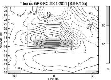
3 Quantification of observed temperature variability 3.1 Observed temperature variability in the TTL Figure 2 shows the latitude–height section of the linear tem-perature trends for the period 2001–2011 estimated from GPS-RO observations (see details of the GPS-RO data in Wang et al., 2013). A remarkable and statistically signif-icant warming occurs around the TTL between about 20◦

south to north and from 16 to 21 km height. The warming in the TTL is 0.9 K decade−1 _{on average, with a maximum}

of about 1.8 K decade−1 _{directly at the tropical tropopause}

around 17 to 18 km. This figure is an extension of earlier work by Schmidt et al. (2010) and Wang et al. (2013) and shows an unexpected warming, despite the steady increase in GHGs. Therefore it is interesting to study whether this warm-ing is simply a phenomenon of the past decade and the result of internal atmospheric variability, or whether it will persist for longer and therefore modify trace gas transport from the troposphere into the stratosphere.

(6)

T trends GPS-RO 2001-2011 [ 0.9 K/10a]

-30 0 30

Latitude 10 11 12 13 14 15 16 17 18 19 20 21 22 23 24 25

Altitude (km) 90

95

% 90 95

-30 0 30

Latitude 10 11 12 13 14 15 16 17 18 19 20 21 22 23 24 25 Altitude (km)

T trends GPS-RO 2001-2011 [ 0.9 K/10a]

-1.0 -0.8 -0.6 -0.4

-0.4 -0.2 -0.2 0.0 0.0 0.0 0.0 0.2 0.2 0.2 0.2 0.4 0.4 0.4 0.4 0.6 0.6 0.6 0.8

1.0 1.2

1.4 1.6

Figure 2.Latitude–height section of linear temperature trends over the past decade (2001–2011) from GPS-RO data over a height range

from 10 to 25 km and 35◦_{S to 35}◦_{N latitude; contour interval is}

0.2 K decade−1. Grey shading represents the statistical significance

for the trends.

still very important to understand the reasons and mecha-nisms behind these internal variability modes as it might eventually enhance our decadal to multi-decadal predictive skills.

3.2 Contribution of solar variability

Figure 3a and b show the correlation between temperature differences (Natural – SolarMean) with solar forcing (TSI) in the Natural run over the whole simulation period from 1955 through 2099, as well as the estimated temperature trends during 2001 through 2011 related to a decreasing TSI. The correlation between temperature differences and TSI is rela-tively weak, amounts to less than 0.1 in the TTL region and is a little higher and more significant in the lower stratosphere. With such a weak positive correlation, the decreasing solar irradiance contributed to a cooling of about 0.2 K decade−1

in the TTL during 2001–2011. 3.3 Contribution of tropical SSTs

Figure 4 shows the correlation between temperature differ-ences (Natural – FixedSST) with tropical (20◦

S–20◦

N) SSTs from the Natural run over the whole simulation period from 1955 through 2099, as well as the estimated temperature trends from 2001 through 2011 due to decreasing tropical SSTs. Temperature differences are closely correlated with tropical SSTs, which show strong positive correlations (up to 0.8) below and significant negative correlations (over 0.5) above the tropopause in the tropics. The strong correlation between tropical SSTs and atmospheric temperatures indi-cates that tropical SSTs have important impacts on the TTL temperature. A decrease in tropical SSTs contributes there-fore to a statistically significant warming of 0.3 K decade−1

(a) Tdiff & Solar Correlation (1955-2099)

-30 0 30

Latitude 11 13 15 17 19 21 23 25 Altitude (km)

90 95

%

-30 0 30

(a) Tdiff & Solar Correlation (1955-2099)

0.0

0.1

(b) Tfac Solar (2001-2011) [-0.2 K/10a]

-30 0 30

90 95

%

-30 0 30

(b) Tfac Solar (2001-2011) [-0.2 K/10a]

-0.2

-0.1

0.0

Figure 3. (a)Latitude–height sections of correlations between tem-perature differences (Natural – SolarMean) and solar TSI in the Natural run over the whole period (1955–2099); contour interval is 0.1; grey shading represents statistically significant correlations,

with Student’sttest.(b)The regressed contributions of solar TSI

to the TTL temperature trends during 2001–2011 (Eq. 2); contour

interval is 0.1 K decade−1_{; grey shading represents statistically}

sig-nificant regressions. See text for details on the calculation of the regressed trend and the testing of the statistical significance. The decadal temperature trend in the title is the mean value from the dashed box.

(a) Tdiff & SST Correlation (1955-2099)

-30 0 30

90 95

%

-30 0 30

(a) Tdiff & SST Correlation (1955-2099)

-0.5 -0.4 -0.3 -0.2 -0.1

0.0 0.1 0.2 0.2 0.2 0.3 0.3 0.3 0.4 0.5 0.6 0.7

(b) Tfac SST (2001-2011) [ 0.3 K/10a]

-30 0 30

90 95

%

-30 0 30

(b) Tfac SST (2001-2011) [ 0.3 K/10a]

-0.4 -0.2 -0.2 -0.2 0.0 0.2

0.4 0.6

Figure 4.Same as Fig. 3 but for the impact of tropical SSTs by

comparing the Natural and FixedSST runs. Contour interval is(a)

0.1 and(b)0.2 K decade−1_.

on average (0.6 K decade−1

in maximum) in the TTL during 2001–2011 (Fig. 4c).

3.4 Contribution of the QBO

As described in Sect. 2.5, a pair of orthogonal time series of the QBO are used in the regression between temperature dif-ferences (Natural – NOQBO) and the QBO from the Natural run. Since the QBO1 mainly affects temperature in the mid-dle and upper stratosphere, only the QBO2 correlation and impacts are shown in Fig. 5. QBO2 features a strong positive correlation in the TTL region, which amounts up to 0.6. An observed increase of QBO2 during 2001–2011, which means stronger westerlies, therefore contributes to a 0.2 K decade−1

warming on average (0.4 K decade−1

(7)

(a) Tdiff & QBO Correlation (1955-2099)

-30 0 30

90 95

%

-30 0 30

(a) Tdiff & QBO Correlation (1955-2099)

-0.4 -0.4 -0.2 -0.2 0.0 0.0 0.0 0.2 0.2 0.2 0.4

(b) Tfac QBO (2001-2011) [ 0.2 K/10a]

-30 0 30

90 95

%

-30 0 30

(b) Tfac QBO (2001-2011) [ 0.2 K/10a]

0.0 0.0

0.0

0.2

Figure 5.Same as Fig. 3 but for the impact of the QBO2 (see text for details) by comparing the Natural and the NOQBO experiments;

contour interval is(a)0.2 and(b)0.2 K decade−1_.

TTL. Another effect of the QBO is the statistically signif-icant cooling trend seen in the tropical middle stratosphere above 23 km. This QBO effect may help to explain the ob-served tropical cooling (see Fig. 2). However, CESM1.0 used for these simulations cannot generate a self-consistent QBO and hence uses wind nudging, which might cause problems when estimating QBO effects on temperature variability in the tropical lower stratosphere (Marsh et al., 2013; Morgen-stern et al., 2010).

3.5 Contribution of GHGs

As expected, GHGs show strong positive correlations with temperatures in the troposphere and significant negative cor-relations with temperatures in the stratosphere, with a switch of sign near the tropopause (about 18 km, Fig. 6a). Increasing GHGs in the RCP85 experiment tend to cool the lower strato-sphere and warm the upper tropostrato-sphere, but have no evident contribution around the tropopause (with a change of corre-lation sign at about 18 km, Fig. 6b). This is consistence with previous studies (e.g. Kim et al., 2013), which confirmed a warming at 100 hPa (below the tropopause) and a cooling at 70 hPa (above the tropopause) due to the increase of GHGs in CMIP5 (Coupled Model Intercomparison Project Phase 5) simulations.

3.6 Contribution of stratospheric aerosols

The correlations between temperature differences (W_Aerosol – W_L103) with CCMI stratospheric aerosols, as well as the contributions of increasing stratospheric aerosols to the recent warming in the TTL are shown in Fig. 7a and b respectively. Weak but partly significant correlations of stratospheric aerosols to temperature in the TTL can be found in Fig. 7a, with a change of correlation sign below the tropopause (about 15 km) and up to 0.2 in the lower stratosphere. The effect of increasing stratospheric aerosols during 2001–2011 is estimated to be 0.2 K decade−1

(a) Tdiff & GHG Correlation (1955-2099)

-30 0 30

90 95

%

-30 0 30

(a) Tdiff & GHG Correlation (1955-2099)

-0.8 -0.6 -0.4_-0.2

0.0 0.2 0.4_0.6

0.8

(b) Tfac GHG (2001-2011) [ 0.0 K/10a]

-30 0 30

90 95

%

-30 0 30

(b) Tfac GHG (2001-2011) [ 0.0 K/10a]

-0.1

0.0

0.1

0.2

Figure 6.Same as Fig. 3 but for the impact of anthropogenic forc-ings (GHGs) by comparing the Natural and RCP85 experiments;

contour interval is(a)0.2 and(b)0.1 K decade−1.

(a) TDiff & Aerosol Correlation (2001-2010)

-30 0 30

90 95

%

-30 0 30

(a) TDiff & Aerosol Correlation (2001-2010)

-0.1 -0.1 0.0 0.1 0.1 0.2 0.2

(b) Tfac Aeorosol (2001-2010) [ 0.2 K/10a]

-30 0 30

90 95

%

-30 0 30

(b) Tfac Aeorosol (2001-2010) [ 0.2 K/10a]

-0.1 0.0 0.1 0.1 0.2 0.2 0.2

Figure 7.Same as Fig. 3 but for the impact of stratospheric aerosols by comparing the W_L103 and the W_Aerosol experiments.

Con-tour interval is(a)0.1 and(b)0.1 K decade−1. The temperatures in

the W_L103 run were calculated from a three member ensemble mean.

warming in the TTL (Fig. 7b). Note that there may exist uncertainties for this result since we have only 10 years of simulations for the W_Aerosol run.

4 Effects of the vertical resolution

To estimate not only anthropogenic and natural contributions to the recent TTL temperature variability but also the effects of the vertical resolution in the model, Fig. 8 shows the tem-perature trends in both the standard (W_L66) and the high vertical resolution (W_L103) runs, as well as their differ-ences. The W_L103 run (Fig. 8b) shows a statistically sig-nificant 0.5 K decade−1 _{warming on average over the past}

decade around the TTL, which maximizes at 1.2 K decade−1_.

(8)

(b) T W_L103 [ 0.5 K/10a]

-30 0 30 Latitude 11 13 15 17 19 21 23 25 Altitude (km)

(b) T W_L103 [ 0.5 K/10a]

-0.6 -0.4

-0.4 -0.2 -0.2 -0.2 -0.2 0.0 0.0 0.0 0.2 0.4 0.6 0.8_1.0 (a) T W_L66 [-0.3 K/10a]

11 13 15 17 19 21 23 25 Altitude (km) 90 95 % 90 95 11 13 15 17 19 21 23 25 Altitude (km)

(a) T W_L66 [-0.3 K/10a]

-1.2

-1.0_-0.8 -1.0

-0.8

-0.6 _-0.6

-0.4

-0.4 -0.2

-0.2

0.0 0.0

0.0

(c) T W_L103-W_L66 [ 0.8 K/10a]

-30 0 30 Latitude

(c) T W_L103-W_L66 [ 0.8 K/10a]

0.0 0.0

0.2 0.4 0.4 0.6 0.6 0.8 1.0

Figure 8. (a, b) Latitude–height sections of temperature trends over 2001–2010 from the W_L103 and W_L66 experiments

respec-tively.(c)The differences between(a)and(b). Contour interval is

0.2 K decade−1and grey shading represents statistically significant

trends. The temperature trends in the W_L103 and W_L66 runs are calculated by multiple linear regression for each three simulations.

(Fig. 8c). Wang et al. (2013) showed that the tropical up-welling in the lower stratosphere has weakened over the past decade in the W_L103 run, while there is no significant up-welling trend in the standard vertical resolution (W_L66) run. The decreasing tropical upwelling in the W_L103 run might be the reason for the extra warming in the TTL com-pared to the W_L66 run, since dynamical changes would lead to adiabatic warming. More detailed investigations will be given in the following section.

4.1 Changes in the Brewer–Dobson circulation

To investigate dynamical differences between the two exper-iments with standard and higher vertical resolution in more detail, the transformed Eulerian mean diagnostic (Andrews et al., 1987) was applied to investigate differences in the wave propagation and BDC in the climatological mean as well as in the decadal trend.

Figure 9 shows the annual mean climatology of the BDC (arrows for the meridional and vertical wind components), the zonal mean zonal wind (blue contour lines) and the tem-perature (filled colours) from the W_L103 run (Fig. 9a), as well as the differences between the W_L103 and the W_L66 runs (Fig. 9c). The BDC shows an upwelling in the trop-ics and a downwelling through middle to high latitudes in the annual mean. With finer vertical resolution (W_L103)

(b) Tr W_L103

−30 0 30

10 12 14 16 18 20 22 24

(a) W_L103 Clm

10 12 14 16 18 20 22 24

(d) Tr L103−L66

−30 0 30

(c) L103−L66 Clm

0.03 0.1 0.01 0.01 −0.8 −0.6 −0.4 −0.2 0 0.2 0.4 0.6 0.8 1 1.2 1.4 195 200 205 210 215 220 225 230 235 240 245 −0.8 −0.6 −0.4 −0.2 0 0.2 0.4 0.6 0.8 1 1.2 1.4 −1.5 −1 −0.5 0 0.5 1 1.5 2 2.5 3 3.5 4

Figure 9. (a)Annual mean climatological zonal mean zonal wind

(contours; contour interval is 10 m s−1_{; dashed lines indicate}

east-erly winds), BDC vector (arrows, scaled with the square root of pressure) and temperature (colour shadings) for the W_L103

exper-iment from 8 to 25 km and 35◦S through 35◦N.(c)Differences of

the zonal mean zonal wind (contour interval 1.0 m s−1_{), BDC}

vec-tor and temperature (colour shadings indicate 95 % statistical

sig-nificance) between the W_L103 and the W_L66 experiments.(b)

and(d)are the same as(a)and (c)but for the linear trends from

2001 to 2010. The shadings in(b)and(d)indicate 95 % statistical

significance. The contour intervals are 2 and 1 m s−1_in_(c)_and_(d)

respectively.

the model produces a stronger upwelling in the tropics (and a consistent cooling) up to the tropopause region, with west-erly wind anomalies above. This strengthened tropical up-welling cannot continue further up because of the westerly wind anomalies which block the transport into the subtropics (Simpson et al., 2009; Flannaghan and Fueglistaler, 2013). Above the tropical tropopause there is less upwelling and in particular more transport from the subtropics into the trop-ical TTL, leading to a stronger warming around 19 km in the W_L103 experiment. These changes in the BDC indicate a strengthening of its lower branch and a weakening at up-per levels in the lower stratosphere (Lin and Fu, 2013). This is consistent with a previous work by Bunzel and Schmidt (2013) which indicates a weaker upward mass flux around 70 hPa in a model experiment with higher vertical resolution. The annual mean trends in the W_L103 experiment indi-cate a further strengthening of the BDC lower branch over the past decade in this simulation (Fig. 9b) and a statistically significant weakening in the lower stratosphere resulting in significant warming of 1 to 2 K decade−1_{in the TTL. In}

par-ticular the trends in the TTL are stronger in the W_L103 compared to the W_L66 experiment (Fig. 9d).

(9)

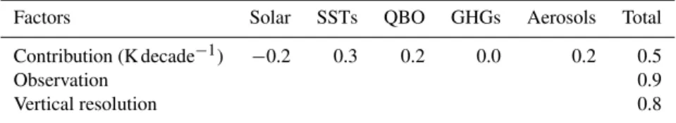
Table 3.Summary of contributions from the varying factors to the observed TTL warming between 2001 and 2011, in the region 20◦_S–20◦_N latitude and 16–20 km.

Factors Solar SSTs QBO GHGs Aerosols Total

Contribution (K decade−1₎ ₋_0.2 _0.3 _0.2 _0.0 _0.2 _0.5

Observation 0.9

Vertical resolution 0.8

of the BDC in the lower stratosphere. These changes in the BDC and corresponding wave–mean flow interactions (not shown) finally result in the statistically significant warming in the TTL.

Bunzel and Schmidt (2013) attributed the differences in the BDC to different vertical resolutions which tend to re-duce the numerical diffusion through the tropopause and the secondary meridional circulation. Our results show that the strong warming and subsequent enhanced static stability (not shown) above the tropopause may also influence wave dissi-pation and propagation around the tropopause. Oberländer et al. (2013) point out that an increase of tropical SSTs en-hances the BDC. This is consistent with our results, which show a weakening of the BDC in the lower stratosphere fol-lowing a decrease in tropical SSTs. At the same time, this response of the stratosphere to the surface can be better rep-resented by a model with finer vertical resolution.

5 Summary and discussion

Based on a series of sensitivity simulations with NCAR’s CESM-WACCM model, the relationships between differ-ent natural (solar, QBO, tropical SSTs) and anthropogenic (GHGs, ODS) factors and temperatures around TTL, as well as their contributions to the observed warming of the TTL over the past decade from 2001 through 2011, have been studied. By regressing the temperature differences between model experiments to the respective factors for the whole simulation periods between 1955 and 2099 and projecting the regressed coefficients onto the observed trends of the re-spective factor during 2001–2011, the contribution of each factor has been quantified in order to explain the causes of the observed recent decadal variability seen in GPS-RO data. The SSTs show strong significant negative correlation (−0.5) with temperatures in the TTL, while the QBO2 shows a reversed pattern (0.6). The TSI and stratospheric aerosols result in weak positive correlations (0.1–0.2) with TTL tem-peratures. GHGs show positive correlations with tempera-tures in the troposphere and negative correlations with tem-peratures in the stratosphere, while there is no significant cor-relation around the tropopause.

A decrease in tropical SSTs, an increase in stratospheric aerosol loading and stronger QBO westerlies contribute each about 0.3, 0.2 and 0.2 K decade−1 _{to this warming}

respec-tively, resulting in a total 0.7 K decade−1

warming, while the

delay and smaller amplitude of the current solar maximum contribute about 0.2 K decade−1_{to cooling. Adding all}

natu-ral and anthropogenic factors, we estimate a total modelled warming of 0.5 K decade−1_{around the TTL (Table 3), which}

is less than the observed 0.9 K decade−1_{warming from}

GPS-RO data. One possible reason of this weak estimate is the relative low vertical resolution of the model, which strongly influences the TTL response to the surface mainly via dy-namical changes, i.e. an enhancement of the lower branch of the BDC and a decrease of the upper branch in the lower stratosphere in response to decreasing tropical SSTs. This leads to a 0.8 K decade−1 extra warming in the TTL in the finer vertical resolution experiment as compared to the stan-dard vertical resolution. However, in reality non-linear inter-actions between the different factors occur which we did not take into account in our first-order linear approach. The com-prehensive impact of all factors on the recent TTL warming can be estimated by the W_Aerosol run. The W_Aerosol run, with almost all observed forcings considered in this study, can be seen as the most realistic simulation. The TTL warm-ing in the W_Aerosol run is on average 0.9 K decade−1_and

maximum 1.6 K decade−1_{(Fig. 7b), both of which are very}

close to the observed trend.

According to our experiments, one of the primary factors contributing to the recent warming in the TTL is the natu-ral variability in tropical SSTs. However, the mechanism of the TTL response to SSTs awaits further investigation. One key issue is how much improvement we can expect from using a fully coupled ocean–atmosphere model instead of atmosphere-only model with prescribed SSTs. Our W_L66 and W_L103 simulations indicate that the atmosphere-only model may not correctly reproduce the response of TTL vari-ability to SST, but can be improved with finer vertical reso-lution.

Another important factor in contributing to the recent warming in the TTL is the QBO. The QBO is closely related to the tropical upwelling Flury et al. (2013). A regression of temperature differences onto the differences in the vertical component of BDC between the Natural and NOQBO run shows a very similar result than the regression of tempera-ture differences onto the QBO time series (not shown). The QBO may influence the TTL temperature by modifying the BDC.

(10)

Era Retrospective-analysis for Research and Applications (MERRA) reanalysis data and our Natural and RCP85 runs, which provide strong support to the internal variability dom-inated TTL warming over the past decade.

The external forcings (solar, GHGs, ODS) contribute rel-atively little to the temperature variability in the TTL, ex-cept for the stratospheric aerosols. Internal variability, i.e. the QBO and tropical SSTs, seem to be mainly responsible for the recent TTL warming.

The Supplement related to this article is available online at doi:10.5194/acp-15-5815-2015-supplement.

Acknowledgements. W. Wang is supported by a fellowship of the China Scholarship Council (CSC) at FU Berlin. This work was also performed within the Helmholtz University Young Investigators Group NATHAN, funded by the Helmholtz Association through the president’s Initiative and Networking Fund and the GEOMAR – Helmholtz-Zentrum für Ozeanforschung in Kiel. The model calculations have been performed at the Deutsche Klimarechen-zentrum (DKRZ) in Hamburg, Germany. We thank F. Hansen, C. Petrick, R. Thiéblemont and S. Wahl for carrying out some of the simulations. We appreciate discussions about the statistical methods with D. Maraun and the help with grammar checking from L. Neef.

The article processing charges for this open-access publication were covered by a Research

Centre of the Helmholtz Association.

Edited by: P. Haynes

References

Andrews, D. G.: An Introduction to Atmospheric Physics, Cam-bridge University Press, New York, 248 pp., 2010.

Andrews, D. G., Holton, J. R., and Leovy, C. B.: Middle Atmo-sphere Dynamics, vol. 40, Academic Press, San Diego, 489 pp., 1987.

Baldwin, M. P., Gray, L. J., Dunkerton, T. J., Hamilton, K., Haynes, P. H., Randel, W. J., Holton, J. R., Alexan-der, M. J., Hirota, I., Horinouchi, T., Jones, D. B. A., Kin-nersley, J. S., Marquardt, C., Sato, K., and Takahashi, M.: The quasi-biennial oscillation, Rev. Geophys., 39, 179–229, doi:10.1029/1999RG000073, 2001.

Bourassa, A. E., Robock, A., Randel, W. J., Deshler, T., Rieger, L. A., Lloyd, N. D., Llewellyn, E. T., and Degen-stein, D. A.: Large volcanic aerosol load in the stratosphere linked to Asian monsoon transport, Science, 337, 78–81, doi:10.1126/science.1219371, 2012.

Bunzel, F. and Schmidt, H.: The Brewer–Dobson circulation in a changing climate: impact of the model configuration, J. Atmos. Sci., 70, 1437–1455, doi:10.1175/JAS-D-12-0215.1, 2013.

Butchart, N.: The Brewer–Dobson circulation, Rev. Geophys., 52, 157–184, doi:10.1002/2013RG000448, 2014.

Butchart, N., Cionni, I., Eyring, V., Shepherd, T. G., Waugh, D. W., Akiyoshi, H., Austin, J., Bruhl, C., Chipperfield, M. P., Cordero, E., Dameris, M., Deckert, R., Dhomse, S., Frith, S. M., Garcia, R. R., Gettelman, A., Giorgetta, M. A., Kinnison, D. E., Li, F., Mancini, E., McLandress, C., Pawson, S., Pitari, G., Plummer, D. A., Rozanov, E., Sassi, F., Scinocca, J. F., Shibata, K., and Tian, W.: Chemistry-climate model simulations of twenty-first century stratospheric climate and circulation changes, J. Climate, 23, 5349–5374, doi:10.1175/2010JCLI3404.1, 2010.

Dessler, A. E., Schoeberl, M. R., Wang, T., Davis, S. M.,

and Rosenlof, K. H.: Stratospheric water vapor

feed-back, P. Natl. Acad. Sci. USA, 110, 18087–18091,

doi:10.1073/pnas.1310344110, 2013.

Dessler, A., Schoeberl, M., Wang, T., Davis, S., Rosenlof, K., and Vernier, J.-P.: Variations of stratospheric water vapor over the past three decades, J. Geophys. Res., 119, 12–588, doi:10.1002/2014JD021712, 2014.

Engel, A., Mobius, T., Bonisch, H., Schmidt, U., Heinz, R., Levin, I., Atlas, E., Aoki, S., Nakazawa, T., Sugawara, S., Moore, F., Hurst, D., Elkins, J., Schauffler, S., Andrews, A., and Boering, K.: Age of stratospheric air unchanged within uncertainties over the past 30 years, Nat. Geosci., 2, 28–31, doi:10.1038/ngeo388, 2009.

Flannaghan, T. and Fueglistaler, S.: The importance of the tropi-cal tropopause layer for equatorial Kelvin wave propagation, J. Geophys. Res., 118, 5160–5175, doi:10.1002/jgrd.50418, 2013. Flury, T., Wu, D. L., and Read, W. G.: Variability in the speed

of the Brewer–Dobson circulation as observed by Aura/MLS, Atmos. Chem. Phys., 13, 4563–4575, doi:10.5194/acp-13-4563-2013, 2013.

Fueglistaler, S., Dessler, A., Dunkerton, T., Folkins, I., Fu, Q., and Mote, P. W.: Tropical tropopause layer, Rev. Geophys., 47, 1004, doi:10.1029/2008RG000267, 2009.

Fueglistaler, S., Liu, Y., Flannaghan, T., Haynes, P., Dee, D., Read, W., Remsberg, E., Thomason, L., Hurst, D., Lanzante, J., and Bernath, P. F.: The relation between atmospheric humidity and temperature trends for stratospheric water, J. Geophys. Res., 118, 1052–1074, doi:10.1002/jgrd.50157, 2013.

Gettelman, A. and Birner, T.: Insights into tropical tropopause layer processes using global models, J. Geophys. Res., 112, D23104, doi:10.1029/2007JD008945, 2007.

Gettelman, A. and Forster, P. D. F.: A climatology of the trop-ical tropopause layer, J. Meteor. Soc. Jpn., 80, 911–924, doi:10.2151/jmsj.80.911, 2002.

Gettelman, A., Birner, T., Eyring, V., Akiyoshi, H., Bekki, S., Brühl, C., Dameris, M., Kinnison, D. E., Lefevre, F., Lott, F., Mancini, E., Pitari, G., Plummer, D. A., Rozanov, E., Shi-bata, K., Stenke, A., Struthers, H., and Tian, W.: The Tropical Tropopause Layer 1960–2100, Atmos. Chem. Phys., 9, 1621– 1637, doi:10.5194/acp-9-1621-2009, 2009.

(11)

Grise, K. M. and Thompson, D. W.: Equatorial planetary waves and their signature in atmospheric variability, J. Atmos. Sci., 69, 857– 874, doi:10.1175/JAS-D-11-0123.1, 2012.

Grise, K. M. and Thompson, D. W.: On the signatures of equato-rial and extratropical wave forcing in tropical tropopause layer temperatures, J. Atmos. Sci., 70, 1084–1102, doi:10.1175/JAS-D-12-0163.1, 2013.

Hansen, F., Matthes, K., and Gray, L.: Sensitivity of strato-spheric dynamics and chemistry to QBO nudging width in the chemistry-climate model WACCM, J. Geophys. Res., 118, 10– 464, doi:10.1002/jgrd.50812, 2013.

Kawatani, Y. and Hamilton, K.: Weakened stratospheric quasibi-ennial oscillation driven by increased tropical mean upwelling, Nature, 497, 478–481, doi:10.1038/nature12140, 2013. Kim, J., Grise, K. M., and Son, S.: Thermal characteristics of the

cold-point tropopause region in CMIP5 models, J. Geophys. Res., 118, 8827–8841, doi:10.1002/jgrd.50649, 2013.

Lean, J., Rottman, G., Harder, J., and Kopp, G.: SORCE contribu-tions to new understanding of global change and solar variability, Sol. Phys., 230, 27–53, doi:10.1007/s11207-005-1527-2, 2005. Li, F., Austin, J., and Wilson, J.: The strength of the

Brewer–Dobson circulation in a changing climate: coupled chemistry-climate model simulations, J. Climate, 21, 40–57, doi:10.1175/2007JCLI1663.1, 2008.

Lin, P. and Fu, Q.: Changes in various branches of the Brewer– Dobson circulation from an ensemble of chemistry climate mod-els, J. Geophys. Res., 118, 73–84, doi:10.1029/2012JD018813, 2013.

Marsh, D. R., Mills, M. J., Kinnison, D. E., Lamarque, J.-F., Calvo, N., and Polvani, L. M.: Climate change from 1850 to 2005 simulated in CESM1 (WACCM), J. Climate, 26, 7372– 7391, doi:10.1175/JCLI-D-12-00558.1, 2013.

Matthes, K., Marsh, D. R., Garcia, R. R., Kinnison, D. E., Sassi, F., and Walters, S.: Role of the QBO in modulating the influence of the 11 year solar cycle on the atmosphere using constant forc-ings, J. Geophys. Res., 115, 18110, doi:10.1029/2009JD013020, 2010.

Meehl, G. A., Washington, W. M., Arblaster, J. M., Hu, A., Teng, H., Tebaldi, C., Sanderson, B. N., Lamarque, J.-F., Conley, A., Strand, W. G., and White, J. B.: Climate system response to ex-ternal forcings and climate change projections in CCSM4, J. Cli-mate, 25, 3661–3683, doi:10.1175/JCLI-D-11-00240.1, 2012. Meinshausen, M., Smith, S. J., Calvin, K., Daniel, J. S., Kainuma,

M. L. T., Lamarque, J.-F., Matsumoto, K., Montzka, S., Raper, S., Riahi, K., Thomson, A., Velders, G. J. M., and van Vuuren, D. P.: The RCP greenhouse gas concentrations and their ex-tensions from 1765 to 2300, Climatic Change, 109, 213–241, doi:10.1007/s10584-011-0156-z, 2011.

Morgenstern, O., Giorgetta, M. A., Shibata, K., Eyring, V., Waugh, D. W., Shepherd, T. G., Akiyoshi, H., Austin, J., Baumgaertner, A. J. G., Bekki, S., Braesicke, P., Brühl, C., Chipperfield, M. P., Cugnet, D., Dameris, M., Dhomse, S., Frith, S. M., Garny, H., Gettelman, A., Hardiman, S. C., Hegglin, M. I., Jöckel, P., Kinnison, D. E., Lamarque, J.-F., Mancini, E., Manzini, E., Marchand, M., Michou, M., Nakamura, T., Nielsen, J. E., Olivié, D., Pitari, G., Plum-mer, D. A., Rozanov, E., Scinocca, J. F., Smale, D., Teyssè-dre, H., Toohey, M., Tian, W., and Yamashita, Y.: Review of the formulation of present-generation stratospheric

chemistry-climate models and associated external forcings, J. Geophys. Res., 115, D00M02, doi:10.1029/2009JD013728, 2010. Neely, R. R., Toon, O. B., Solomon, S., Vernier, J. P., Alvarez, C.,

English, J. M., Rosenlof, K. H., Mills, M. J., Bardeen, C. G., Daniel, J. S., and Thayer, J. P.: Recent anthropogenic increases

in SO2from Asia have minimal impact on stratospheric aerosol,

Geophys. Res. Lett., 40, 999–1004, doi:10.1002/grl.50263, 2013. Oberländer, S., Langematz, U., and Meul, S.: Unraveling impact factors for future changes in the Brewer–Dobson circulation, J. Geophys. Res., 118, 10–296, doi:10.1002/jgrd.50775, 2013. Randel, W. J. and Jensen, E. J.: Physical processes in the

tropi-cal tropopause layer and their roles in a changing climate, Nat. Geosci., 6, 169–176, doi:10.1038/ngeo1733, 2013.

Randel, W. J., Shine, K. P., Austin, J., Barnett, J., Claud, C., Gillett, N. P., Keckhut, P., Langematz, U., Lin, R., Long, C., Mears, C., Miller, A., Nash, J., Seidel, D. J., Thomp-son, D. W. J., Wu, F., and Yoden, S.: An update of observed stratospheric temperature trends, J. Geophys. Res., 114, D02107, doi:10.1029/2008JD010421, 2009.

Richter, J. H., Solomon, A., and Bacmeister, J. T.: On the simula-tion of the quasi-biennial oscillasimula-tion in the Community Atmo-sphere Model, version 5, J. Geophys. Res.-Atmos., 119, 3045– 3062, doi:10.1002/2013JD021122, 2014.

Schmidt, T., Wickert, J., and Haser, A.: Variability of the upper tro-posphere and lower stratosphere observed with GPS radio occul-tation bending angles and temperatures, Adv. Space. Res., 46, 150–161, doi:10.1016/j.asr.2010.01.021, 2010.

Shepherd, T. G. and McLandress, C.: A robust mechanism for strengthening of the Brewer–Dobson circulation in response to climate change: critical-layer control of subtropical wave break-ing, J. Atmos. Sci., 68, 784–797, doi:10.1175/2010JAS3608.1, 2011.

Simpson, I. R., Blackburn, M., and Haigh, J. D.: The role of eddies in driving the tropospheric response to strato-spheric heating perturbations, J. Atmos. Sci., 66, 1347–1365, doi:10.1175/2008JAS2758.1, 2009.

Solomon, S., Rosenlof, K. H., Portmann, R. W., Daniel, J. S., Davis, S. M., Sanford, T. J., and Plattner, G.-K.: Con-tributions of stratospheric water vapor to decadal changes in the rate of global warming, Science, 327, 1219–1223, doi:10.1126/science.1182488, 2010.

Solomon, S., Daniel, J., Neely, R., Vernier, J.-P., Dutton, E., and Thomason, L.: The persistently variable “background” strato-spheric aerosol layer and global climate change, Science, 333, 866–870, doi:10.1126/science.1206027, 2011.

SPARC-CCMVal: SPARC Report on the Evaluation of Chemistry-Climate Models, SPARC Report 5, WCRP-132, WMO/TD-1526, 2010.

Stiller, G. P., von Clarmann, T., Haenel, F., Funke, B., Glatthor, N., Grabowski, U., Kellmann, S., Kiefer, M., Linden, A., Los-sow, S., and López-Puertas, M.: Observed temporal evolution of global mean age of stratospheric air for the 2002 to 2010 period, Atmos. Chem. Phys., 12, 3311–3331, doi:10.5194/acp-12-3311-2012, 2012.

(12)

Wang, W., Matthes, K., Schmidt, T., and Neef, L.: Recent variability of the tropical tropopause inversion layer, Geophys. Res. Lett., 40, 6308–6313, doi:10.1002/2013GL058350, 2013.

Wigley, T.: Appendix A: Statistical issues regarding trends, in: Tem-perature Trends in the Lower Atmosphere: Steps for Understand-ing and ReconcilUnderstand-ing Differences, edited by: Karl, T. R., Has-sol, S. J., Miller, C. D., and Murray, W. L., A Report by Cli-mate Change Science Program and the Subcommittee on Global Change Research, Washington, DC, USA, UNT Digital Library, 129–139, 2006.

Zhou, X.-L., Geller, M. A., and Zhang, M.: Cooling trend of the tropical cold point tropopause temperatures and

its implications, J. Geophys. Res., 106, 1511–1522,