Banks, Liquidity Crises and Economic Growth
∗
Alejandro Gaytan
New York University
Romain Ranciere
New York University and CERAS
This Version: November, 2002
First Draft: August, 2001
ABSTRACT
How do the liquidity functions of banks affect investment and growth at different stages of economic development? How do financial fragility and the costs of banking crises evolve with the level of wealth of countries? We analyze these issues using an overlapping generations growth
model where agents, who experience idiosyncratic liquidity shocks, can invest in a liquid storage
technology or in a partially illiquid Cobb Douglas technology. By pooling liquidity risk, banks play
a growth enhancing role in reducing inefficient liquidation of long term projects, but they may face liquidity crises associated with severe output losses. We show that middle income economies may
find optimal to beexposed to liquidity crises, while poor and rich economies have more incentives to develop a fully covered banking system. Therefore, middle income economies could experience banking crises in the process of their development and, as they get richer, they eventually converge
to afinancially safe long run steady state. Finally, the model replicates the empirical fact of higher costs of banking crises for middle income economies.
–––––––––––––––––––––––––
KEYWORDS: OLG growth models, liquidity, financial intermediation, financial fragility, bank-ing crises.
JEL Codes: E44, G21, O11
∗We are grateful to Debraj Ray, Jess Benhabib, Boyan Jovanovic, Douglas Gale, Jason Cummins, Olivier Jeanne,
1
Introduction.
This paper investigates the relationship between the liquidity roles of banks, financial fragility and economic growth. It integrates the analysis of liquidity crises into the analysis of the long run
growth effects offinancial intermediation.
The development of a banking system to pool liquidity risk allows economies to achieve higher
growth rates and higher long run level of wealth and consumption. We show that financial devel-opment is particularly important for the growth performance of middle-income economies.
However, a banking system may be vulnerable to liquidity crises with potentially large output
and welfare consequences in the short run. We show that sufficiently rich economies can afford the cost of full coverage against the risk of liquidity crises, while middle income economies may find optimal to remain vulnerable in exchange for higher returns and welfare. This explains why middle
income countries exhibit on average higher growth and higher frequency of banking crises.
A large number of empirical studies support the existence of a positive relationship between
financial intermediation and growth. King and Levine [1995] and Beck, Levine and Loayza [2000]
find a positive effect of the relative size of the banking sector, and several measures of financial development on per capita output growth.1 On the other hand, the banking crisis literature has
pointed out the role of financial liberalization and the rapid increase in financial depth as good predictors offinancial crisis.2 Loayza and Ranciere [2001] attempt to reconcile the apparent contra-diction between those two strands of the literature. They show that a long-run positive relationship
betweenfinancial intermediation and output growth can coexist for some countries with a negative short-run relationship, specially for those countries that have sufferedfinancial crises episodes.
1Beck, Levine and Loayza (2000) use an external instruments approach to address the issue of joint endogeneity
betweenfinancial development and growth.
2See for example Demirguc-Kunt and Degatriache [1998 and 2000]; Gourinchas, Landerretche and Valdes [1999];
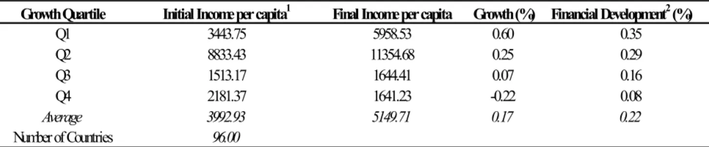
Table 1 : Financial Development and Real Per Capita Income Growth (1975-1998)
Growth Quartile Initial Income per capita1 Final Income per capita Growth (%) Financial Development2 (%)
Q1 3443.75 5958.53 0.60 0.35
Q2 8833.43 11354.68 0.25 0.29
Q3 1513.17 1644.41 0.07 0.16
Q4 2181.37 1641.23 -0.22 0.08
Average 3992.93 5149.71 0.17 0.22
Number of Countries 96.00
1
Real GDP per Capita Constant US$; source: World Development Indicators
2
Financial Development Indicator: Liquid Liabilities / GDP; source: International Financial Statistics
The empirical information on financial development and financial crises provide evidence that the costs and benefits of financial intermediation tend to differ with the level of wealth of the economy. Tables 1 and 2 summarize information on financial development, growth and financial crises.3 Tables 1 orders countries in quartiles according with the real per capita income growth
over the period 1975-1998. For each group, it displays the mean of initial and final income per capita and the degree of variation in financial depth4. Table 1 confirms the positive relationship between growth performance andfinancial development. Moreover, those countries with a joint high performance of growth and financial development are typically middle-income economies who have ”emerged” during the period. At the other end, in the fourth quartile, wefind countries that have experienced declines in per capita income during the period along with poorfinancial development. This suggest thatfinancial intermediation plays a crucial role in the growth performance of middle-income ”emerging” economies.
Table 2 : Real Income Per Capita and Systemic Banking Crises3
Income Quartile Number of systemic banking crisis4 Partition of crises
Q1 6 18.75%
Q2 9 28.13%
Q3 11 34.38%
Q4 6 18.75%
Total 32 100.00%
3
average 1975-1998 GDP per Capita Constant US$
4
source: Caprio and Klingebiel (1999)
3There are 96 countries in the sample from 1975 to 1998. 32 of the countries in this sample experienced at least
one systemic banking crises (Caprio-Klingebiel [1999]).
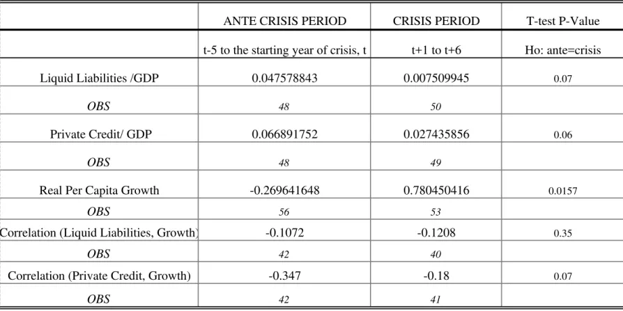
Table 2, presents information on income per capita and banking crises.5 Countries are divided in
quartiles according to their ”level” of GDP per capita. The table shows that the highest frequency
of banking crises is for middle-income economies. Moreover, emerging economies have not only
experienced higher recurrence of banking crises but also more severe costs. Figure 1 plots the
cumulative fiscal cost of banking crises (as percentage of GDP) for countries ranked according to their average per capita income. The severity of the banking crisis has been much higher for
middle-income economies than for poor and rich economies.
F ig u re 1 : F is c a l C o s t o f B a n k in g C ris e s (% G D P )
s o u rc e : C a prio -K lin g eb ie l (1 99 9 )
0 10 20 30 40 50 60
SEN GHA LKA PH
L
CI
V
EGY ECU PRY COL THA BRA URY MEX MYS CHL VEN ARG KOR ESP NZL FI
N FRA SW
E
US
A
NOR
C o u n trie s w ith a b a n k in g c ris is e x p e rie n c e ra n k e d b y In c o m e p e r C a p ita
Financial intermediaries play several roles that can increase depositors’ welfare and foster
eco-nomic growth. This paper focuses only on allocating and liquidity functions of the banks, in
particular: financial intermediaries (i) provide an efficient mechanism that channels investment capital into its higher returns; (ii) are efficient suppliers of liquidity (can transform illiquid assets into liquid liabilities); and (iii) provide liquidity insurance that eliminates idiosyncratic liquidity
5Caprio and Klingebiel define a systemic banking crisis as a situation where aggregate capital of the banking
risk.6 We study what are the costs and benefits of these liquidity functions on welfare and growth of the economy, and how they change in the process of economic development. This paper constitutes,
to our knowledge, the first attempt to study the possibility and consequences of financial crises in a growth model with financial intermediaries.
We use an inter-temporal model of financial intermediaries to analyze the dynamics of wealth, capital and consumption. The model embeds a modified version of the Diamond and Dybvig [1983] model of liquidity provision (henceforth DD)7 into an overlapping generations model (Diamond
[1965]). There are two technologies available, a short term storage technology, and a long term
technology. In this paper, the long run technology uses a standard Cobb-Douglas production
func-tion with labor and capital as inputs. This technology constitutes the channel for growth over time
and among generations.
As it has been noticed by Cooper and Ross [1998], the original Diamond-Dybvig solution does
not consider the impact of the possibility of runs on the design of the optimal deposit contract or
the bank’s investment portfolio. In this paper we characterize the optimal deposit contract offered by a competitive bank when panic runs can occur with positive probability, and we show how
this contract changes with the level of wealth of the economy. When panic crises are possible, an
equilibrium selection mechanism is required. In this paper we consider the simplest mechanism: a
sunspot; we assume that the bank can assign a fixed probability to the event of a panic run. The possibility of bank run occurring with positive probability affects the design of the contract offered by the bank. It involves a decision between being covered, that is, invulnerable to panic runs; and taking the risk to beexposed to liquidity crises. Covered banking is possible at the cost of lower liquidity insurance, while exposed banking has the cost of possible crises episodes. The
welfare implications of these two types of arrangements will depend on the probability with which
crises can happen, and on the level of wealth of the economy.
The characterization of the optimal banking system constitutes the key result of this paper: for
sufficiently high probabilities of crises, a covered banking system would be optimal for any level of wealth; for lower probabilities, poor and rich economies would opt for a covered banking system,
6Most of the existing literature on financial intermediation and growth focus on other functions of financial
intermediation: Pooling of risk among different investment projects, specialization, adoption of new technologies, etc. See for example Greenwood and Jovanovic [1990], Saint Paul [1992] and Acemoglou and Zilibotti [1997].
7The modified version of the Diamond-Dybvig model emphasizes the distinction between liquidity insurance and
while middle income economies would chose an exposed banking system; finally, when the risk of runs is small enough, poor and middle income economies will choose to be exposed to liquidity
crises. Nevertheless as long as the probability of runs is positive, there will be a level of wealth
above which a covered banking system would be optimal.
The analysis of the optimal banking system has important implications for economic growth.
Those economies that choose an exposed banking system take on the risk of short run output losses
of crises to enjoy the higher liquidity insurance and possible higher returns. Nevertheless, as they
get richer, they can eventually ”escape”financial vulnerability and converge to a long runfinancially safe steady state.
The comparison of optimal banking and the benchmark of autarky yields two results. First, the
optimal banking system always dominates autarky in terms of welfare of the current generation of
depositors independently of the probability of runs. Second, even if at early stages of economic
development, the provision of liquidity insurance imposes some growth costs, once the economy
has crossed a certain wealth threshold, the development of a banking system has unambiguously
positive growth consequences.
Finally, we show that the output losses suffered by an exposed system in case of a run, are more severe for middle income economies than for poor and rich economies replicating the empirical
pattern on the costs of banking crises(see Figure 1).
Some previous literature has studied liquidity provision by financial intermediaries in an in-tertemporal framework. In particular, Bencivenga and Smith [1991, 1998], Qi [1994] and Fulghieri
and Rovelli [1998] have studied the DD model in overlapping generations frameworks. Bencivenga
and Smith [1991] investigate the relationship between financial intermediation and growth. How-ever, their model is an endogenous growth model with constant returns to capital. With this
assumption, the role of financial intermediation is no longer dependent on the level of wealth, and
financial intermediation is always growth enhancing. Qi [1994] and Fulghieri and Rovelli [1998] focus is on intergenerational transfers and not on growth; their model has technologies with
con-stant returns to capital and is an endowment economy without dynamics in wealth and no capital
accumulation.8 Even when these authors recognize the presence and potential importance of a bank
8In our model, the use of a Cobb-Douglas technology, for the long asset, makes the returns to investment
run equilibrium, none of these models incorporatefinancial crises in their analysis.
Our results of the mapping between the level of development and the vulnerability to crises have
some similarities with Acemoglu and Zilibotti [1997]. In their model, uncertainty is suppressed above
a certain level of wealth through full diversification, while in our model a sufficiently rich economy can afford the cost of full coverage against crises
Section 2 describes the general set up of the model: the structure of overlapping generations, the
preferences, and the technologies available. Section 3 studies the optimal investment portfolio and
growth underfinancial autarky. Section 4 characterizes the optimal banking system and studies the distortions generated by the possibility of crises and the dynamic implications of banking. Section
5 analyzes the consequences of a banking system, first by comparing the economy with a banking system with the economy under autarky, and then by analyzing the output cost of banking crisis.
Finally, section 6 confronts our results to the empirical evidence, concludes and sets an agenda for
future research.
2
The Basic Model
The economy consists of an infinite sequence of overlapping generations. In each period, a gener-ation, composed by a continuum of ex-ante identical agents with unit mass, is born; there is no
population growth.
Agents live for two periods. They have an endowment of one unit of labor during the first period of their lives, which they supply inelastically. Agents do not value consumption when they
are young. During the second period of their life they are subject to a time preference shock. With
probability π, an agent only values consumption when middle aged (the beginning of her second
period), and becomes an early consumer. With probability (1−π), she only values consumption when old (the end of her second period) and becomes alate consumer. The shock is stochastically independent across agents, and is private information to the agent. Therefore, preferences of an
agent that belongs to generationt are:
U¡ctt, ctE, ctL¢ =Γu¡ctE¢+ (1−Γ)u(ctL) (1)
with
Γ= 1
Γ= 0
with probability π
wherect
E, ctL≥0, are the levels of early and late consumption respectively att+ 1 of an agent born att, andu(·) belongs to the constant relative risk aversion class of utility functions: u(c) = c11−−σσ.
Risk averse agents would like to reduce the ex-ante gap between early and late consumption. We can measure the level of liquidity insurance attained by afinancial arrangement by the ratio of consumptions (cE
cL).
There is one good, used for consumption and investment. There are two technologies available.
A storage technology, that uses the good as unique input and, for each unit invested at t, gives a
return of one unit in any sub-period of t+ 1. There is also a long term technology with a Cobb-Douglas production function, which uses laborl and capitalk as inputs.9 It is assumed that capital
fully depreciates after being used in production. If the technology is left until full maturity (the
end of the period), it gives the return:
z(k, l) =Akβl1−β (2)
Since the unit of labor is supplied inelastically, define the capital intensive production function by:
f(k)≡z(k,1) =Akβ
This production can be prematurely liquidated, with a liquidation cost. In this case the product
generated is a fraction 0< γ < 1 of the full return at maturity, i.e.,γf(k). Hence, the liquidation cost of the long term technology is expressed in terms of output and not in terms of capital. This
assumption makes the relative marginal returns of a long project left until maturity and liquidated
prematurely a constant (γff00(k(k)) ≡ 1 γ).
10
An example helps to better illustrate this liquidation technology. We can think about this
technology as a crop. It is irreversible in terms of the original capital invested (seeds). If it is left
until full maturity, it yields the maximum size of crop; however, premature liquidation would yield
9To motivate the differences of the two technologies, we can think that the country is a small open economy with
access to domestic production (the long technology) and to an international asset (the short technology) that has constant returns to investment (see Velasco and Chang [2000]).
10The results of the paper are robust to a broad range of specifications about concavity of the two technologies.
crop that is not fully grown. Finally, the amount of labor required both at the planting and at the
harvest is the same, and it is independent of the timing of the harvest.
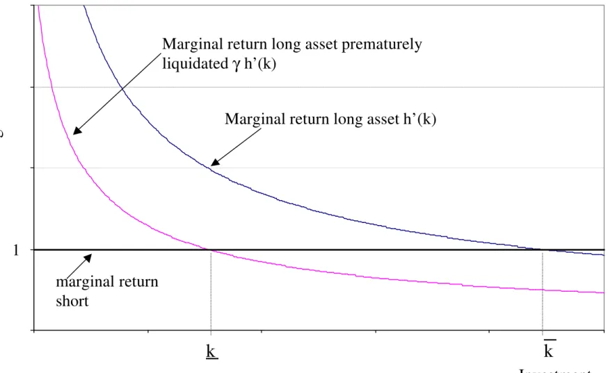
Define the return of holding the long asset as the function h(k) ≡ βf(k). Hence, the marginal return of the long investment ish0(k)if the investment is maintained until full maturity, andγh0(k)
if it is liquidated prematurely. Let’s define the two following capital levels: k such that γh0(k) = 1
k such that h0(k) = 1
Since labor is inelastically supplied, the long term asset presents diminishing returns to capital.
Figure 2 describes the marginal returns of the technologies as functions of the level of investment. For
low levels of capital (k < k), the marginal return of the long term asset, even when it is prematurely
liquidated, exceeds the marginal return of the storage technology (γh0(k)≥1). Beyond some level
of investment in the long asset (k > k), its marginal return is lower than one (h0(k)≤1)
Factor markets are competitive, so each input is paid its realized marginal product. However,
the realized marginal product depends on thefinancial arrangement in place because it depends on the proportion of long term projects liquidated.
Wages received at the end of period t represent the unique source of wealth for members of
the generation. After receiving wages, agents realize make investment decisions before observing
the realization of their liquidity shock. Since agents do not value consumption when young, the
consumption-saving decision at t is trivial, and they will invest their full wealth either directly in
the two technologies (autarky) or as bank deposits (financial intermediation).11 It is assumed that there is an initial generation endowed withw0 >0units of the consumption good.
In the two following sectiona we set up two financial arrangements: financial autarky and the competitive banking solution. Financial autarky is a benchmark to compare the welfare and growth
costs and benefits offinancial intermediation. In this case, agents have to insure themselves against future liquidity needs. In the second case we develop a general banking solution, where thefinancial intermediary provides liquidity and liquidity insurance to depositors. Under this arrangement,
the idiosyncratic liquidity shock is private information to the agent, and the bank has to offer incentive compatible allocations. However, even when a truth revelation mechanism is in place,
11This is an importan difference from the OLG model of Diamond (1965). We abstract from the
panic bank runs are still possible, and the optimal demand deposit contract must consider the
bank’s expectations about the probability of a panic.
3
Financial Autarky
Under financial autarky, young agents make their investment decision between storing goods and investing in capital on their own. We adopt a simplifying assumption about the structure of the
economy. We assume that each worker supplies her unit of labor to a continuum of representative
firms with massm ∈ (0,1].12. With this assumption, young workers are paid a wage equal to the expected marginal product of labor wt+1 = (1−β) [πγ+ 1−π]f(kt)13 and, at the same time, the investors (old agents) receive the marginal product of their investment-liquidation decision (γβf(k)
if early consumer and βf(k)if late).
3.1
The optimal individual investment decision
In the absence offinancial markets, agents cannot get insurance against idiosyncratic liquidity risk. Investment in capital is risky in the sense that its return will depend on the realization of the
liquidity shock. Agents’ investment choices will determine the level of consumption they will enjoy
under each state of nature . At the end of theirfirst period, for any given level of wealthw >0, a typical agent of generationt, chooses investment in the long technology k to maximize:
πu(cE) + (1−π)u(cL) (3)
subject to 0≤k≤w (4)
wherecE =w−k+γh(k), cL =w−k+h(k), and the difference between wealth and capital (w−k), represents investment in the storage technology.
The following proposition characterizes the optimal solution for members of any given generation
under financial autarky:
12This massmcan be arbitrarily close to zero, however, it is equivalent to assume that every worker works for all firms.
13This assumption avoids the possibility of heterogeneity among consumers, that would unnecessarily complicate
Proposition 3.1
w u0(cE)
u0(cL) k cE cL
I 0< w ≤w∗ γ1σ k =w γh(w) h(w)
II w≥w∗ u0(c
E) u0(cL) =
(1−π)(h0(k)−1)
π(1−γh0(k)) k =k
a(w) w−k+γh(k) w−k+h(k)
with w∗ defined by: h0(w∗) = π+(1−π)γσ γπ+(1−π)γσ
Proof. Gaytan—Ranciere (2002a).
The optimal solution under autarky is inefficient. The source of inefficiencies is that, in the absence offinancial markets, each agent needs to insure herself against any liquidity need she may face. In poor economies self insured agents invest, as precautionary savings, their full wealth in
capital beyond the point where it is efficient to do so. When the marginal return of the short asset exceeds the marginal liquidation value of the long asset, (γh0(w)<1), it would be efficient to start
investing a fraction of wealth in the short asset. However,w∗ > k means that for any level of wealth
between k andw∗ agents are over-investing in the long asset (k=w), although γh0(w)<1.
For levels of wealth greater than the thresholdw∗, a second inefficiency arises. Early consumers
are forced to liquidate productive investments to cover their liquidity needs, while late consumers
finance some of their consumption by using the less productive liquid investment. The impossi-bility of receiving insurance through financial markets generates an inefficient liquidation of the long investment. Therefore, when w is very large investment in capital is bounded above by kmax
(h0(k
max) = πγ+(11−π) >1), while it is efficient to invest up to the higher level k (h0
¡
k¢= 1)14. For low levels of wealth, when agents are investing only in the long technology, liquidity self
insurance is constant (cE
cL =γ). For higher levels of wealth, when agents are investing in both assets
(w > w∗), an increase in wealth reduces the gap between early and late consumption. Nevertheless,
full liquidity risk insurance is not possible under financial autarky.
3.2
The dynamics of wealth, capital and consumption under autarky
We can now characterize the steady state of the economy and study the evolution of wages, capital
and consumption towards this stationary equilibrium. Since capital fully depreciates after it is
14Notice that our analysis of the inefficiency of financial autarky echoes the literature on precautionary savings
used, the connection between the individual problem and the dynamics of the intertemporal model
is given by wages of the next generation:
wt=Fa(wt−1) = (1−β)(πγ+ 1−π)f(k(wt−1)) (5) kt=k(wt−1) =kopt(wt−1)
The following proposition characterizes the dynamics of this economy :
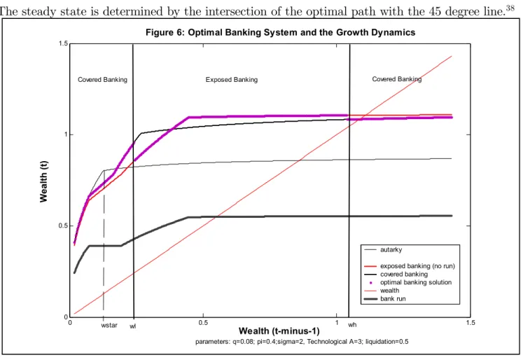
Proposition 3.2 (convergence and the steady state) The economy converges towards a unique stable steady state w_a>0 and k(w_a). The steady state is defined by Fb(w_a) =w_a
Proof. Gaytan-Ranciere (2002a)
Figure 6 presents the dynamics of wealth under autarky. Beyond the threshold w∗, the rate of
growth decreases rapidly, overinvestment in the previous region has already exhausted the marginal
returns on capital. A constant level of liquidationπ,due to self insurance, becomes more and more
costly in terms of growth. Finally, as both consumptions (cE, cL) are monotonically increasing in
wealth, their dynamics follow the dynamics of wealth.
4
Intra-generational Risk Sharing: the Optimal Banking
System
All liquidity uncertainty in this economy pertains to the liquidity needs of individuals, and it is
idio-syncratic. Therefore, welfare gains are possible via a mechanism of liquidity preference insurance.
In addition, underfinancial autarky the mismatch betweenex-post liquidity needs of the agents and the timing of highest returns of the assets, generates an inefficient allocation of aggregate resources. Financial intermediaries can provide welfare improvements by pooling liquidity needs and by fi nd-ing an efficient balance between the agents’ preference for insurance and the timing of the highest returns on the assets.
However, since liquidation is costly, if the value of the bank’s assets at the early sub-period
cannot cover a total withdraw on deposits, the bank is vulnerable to a panic run. Afinancial crisis driven by a panic appears as a coordination problem in which late consumers believe that the bank
won’t be able to service all deposits in the late sub-period, driving a total run on the bank at the
The bank faces a tension between improving welfare of depositors, by offering higher returns and liquidity insurance, and having a more vulnerable system. If the bank could assign a probability to
the event of afinancial panic, it couldfind the most efficient balance between these two objectives. Diamond and Dybvig (1983) does not consider the effect of the possibility of bank runs on the optimal risk sharing contract and the optimal portfolio of the bank. Nevertheless the DD solution
is a benchmark because it is the best risk sharing possible if the liquidity shocks were observable.
We will refer to the DD contract and investment portfolio as thefirst best orunconstrained optimal risk sharing solution.
In this section we develop the optimal risk sharing solution when the bank assigns a fixed probability to a financial panic. The unconstrained optimal risk sharing appears as a limiting case of the general problem (in the limit when the probability of a panic tends to zero). This benchmark
is useful to determine the distortions generated by the existence of unobservable shocks and the
existence of a positive probability of afinancial panic.15
4.1
Generation
t’s
Optimal Risk-Sharing
We consider a generational bank that pools resources and maximizes expected utility of current
depositors. Since the t-bank pools labor income from the agents w, on the aggregate, all liquidity uncertainty disappears: by the law of large numbers, the bank knows that a proportionπ of agents
will demand their deposits in the early sub-period, and a proportion (1−π) in the late sub-period. Therefore it can offer a deposit contract that promises a fixed payment cE for the beginning of periodt+ 1,andcL for the late sub-period oft+ 1. To provide the optimal risk sharing contract the financial intermediary chooses the investment portfoliok, and the optimal liquidation policy. Since the relative marginal returns of the assets vary with the level of wealth, it may be optimal to transfer
resources between sub-periods: the bank can liquidate a proportion λ of the long asset, to serve
early consumers, and it can keep in storage an amountiof the short asset, or ”excess liquidity”, for late consumption. This policy is aimed to form the most efficient match between liquidity needs of agents and the highest returns of the assets. Since the type of agent remains private information,
a self-revelation mechanism is necessary to make the contract incentive compatible. Whenever the
15In our model all the ongoing projects arefinanced with investment of the older generation alive, therefore any
contract offers higher consumption in the late sub-period (cE ≤cL), patient agents have an incentive to wait until the full realization of the assets’ returns.
Existence of a Bank Run Equilibrium
At the beginning oft+ 1those agents that claim to be early consumers withdraw their deposits, and the bank is forced to liquidate any amount of assets required to satisfy that demand. The
remaining assets are let to mature until the second sub-period to serve late consumers. The
impli-cation of the liquidation cost on the long technology is that the value of the bank’s total portfolio
at the early sub-period, (cR ≡w−k+γh(k)) is lower than the value if the technologies were left to mature as planned (w−k+ (λγ + 1−λ)h(k)). When all consumers withdraw their deposits according with their true type, the bank faces a demand ofπcE in the early sub-period. However if
all late agents misrepresent their type and withdraw early, the bank has to meet a total demand for
resources ofcE. Once late agents have learned their type they face the decision between waiting and
receiving a share of the remaining assets in the late sub-period, or claim to be early and withdraw
their resources from the bank. Whenever the bank has enough resources in the early period to
sat-isfy any withdrawal, the dominant strategy for late consumers is to wait. Therefore, a run strategy
can only be optimal if the value of all liabilities in the early sub-period exceed the liquidation value
of the banks portfolio, that is if:
cE > cR ≡w−k+γh(k) (6)
If (6) holds, and the contract is incentive compatible, there are two possible equilibria: a honest equilibrium where agents withdraw from the bank according with their true type, and a run equi-librium where all agents withdraw their deposits, pretending to be early consumers. In the run equilibrium the bank declares bankruptcy and distributes any remaining assets among claimants
following a bankruptcy rule. Here we will assume as bankruptcy rule a pro-rata distribution of the
assets.16 The pro-rata distribution divides equally the liquidation value of the bank’s assets, among
all claimants. Since it is not possible to distinguish who has misrepresented her type and who has
16There are two main bankrupcy rules: the sequential service rule, and the pro-rata distribution. Under the
sequential service rule, the bank services all early withdrawals the promised pay-offcE up to exhaustion of its assets,
withdrawn according with her real liquidity needs, it is optimal to assign the same consumption to
any consumer that has withdrawn early. In the run equilibrium the bank will provide all consumers
an equal share of its assets cR.
Equilibrium Selection Mechanism.
A maximizing bank must necessarily realize that a contract for which (6) holds makes it
vul-nerable to panic runs, and this fact will affect the design of the contract. The question of how the equilibrium is selected when both equilibria are possible is crucial to determine how it affects the choice of the optimal contract. In the absence of additional uncertainty, it is not clear what
drives expectations about the future solvency of the bank. In this paper we assume the most
ba-sic equilibrium selection mechanism:17 a sunspot. We assume that there is a publicly observable
variable that influences the agents’ level of ”optimism” about the solvency of the bank. Suppose that with probabilityq the variable takes values that lead to a pessimistic assessment about future
solvency. Nevertheless, pessimistic expectations can lead to afinancial crisis only when the bank is vulnerable.
4.1.1 The Bank’s Problem
Letθ∈{0,1}be the state variable of a bank run. Ifθ = 1 late agents withdraw the deposits in the early sub-period, and ifθ = 0all agents make their withdrawals according with their type. Letη be the probability of a bank run given the optimal contract and investment portfolio. If the contract
makes the bank solvent under any circumstance in the early sub-period (cE ≤cR) it is not optimal
to run, even if all other late agents run (η = 0). On the other hand if (6) holds the probability of a bank run is the probability of pessimistic expectations (η=q).
At any periodt, and for any given level of deposits (wealthw >0), a representative bank chooses k, λ, i, cE, cL to maximize expected utility of a representative current depositor:18
17Several authors have studied bank runs as an equilibrium phenomenon (Postlwaite and Vives [1987], Jacklin and
Bhattacharya [1988], Cooper and Ross [1998], Allen and Gale [1998], Golfajn and Valdes [1997]). These papers either assume an exogenous probability of crises, or neglect the possibility of panic-based runs. In a recent paper Goldstein and Pauzner [2001] tackle the problem of equilibrium selection and endogenize the probability of bank runs. Based on the ideas of global games developed by Carlsson and van Damme [1993], and Morris and Shin [1998] the authors show that the existence of aggregate uncertainty and imperfect and asymmetric private information, can select a unique equilibrium in the static DD model.
18The bank centralizes production and pays a wage to the following generation (w0) equal to the realized marginal
V(η, w) = max k,λ,i,cE,cL
(1−η) [πu(cE) + (1−π)u(cL)] +ηu(cR) subject to: (7)
πcE ≤w−k−i+λγh(k) (8)
(1−π)cL+πcE ≤w−k+λγh(k) + (1−λ)h(k) (9)
cE ≤cL (10)
0≤λ ≤1 (11)
0≤k ≤w (12)
0≤i≤w−k (13)
cR =w−k+γh(k) (14)
η =
Pr(θ = 1|k∗, λ∗, i∗, c∗E, c∗L) = 0 ⇔cE ≤cR Pr(θ= 1|k∗, λ∗, i∗, c∗
E, c∗L) =q ⇔cE > cR
(15)
Equation 8 is the resource constraint at the early sub-period of t+ 1; for serving agents with early liquidity needs, the bank can liquidate the short asset (w−k) and a proportion λ of the long
term technology. Equation 9 is the resource constraint at the late sub-period of t+ 1; the bank uses all its remaining assets to serve late consumers. Since agents still have access to the storage
technology, the bank must offer a higher return to patient consumers (the incentive compatibility constraint 10). Finally, the probability of a bank run (equation 15) given the optimal contract is
equal to the sunspot probability if the bank is vulnerable to a crisis, and zero otherwise.
The bank’s problem can be decomposed into two decision problems that provide insights about
the tensions and distortions of the optimal contract generated by the possibility of crises. The bank
can offer two alternative types of contracts. Under thefirst type of contract”covered banking”,the
financial intermediary chooses a contract that makes it invulnerable to crisis (cE ≤ cR ⇒ η = 0). The returns on deposits under this contract are independent of the realization of the sunspot. Under
the second type of contract ”exposed banking”, the bank takes on the risk of having a run on its deposits (cE > cR⇒η=q) .19 For any given level of wealth, the bank determinesfirst the optimal contract for each type and, in the second stage, it selects the type of contract that maximizes
expected utility.20 This second decision is equivalent to choosing the probability with which crisis
19Using the terminology of Cooper and Ross (1998) ”covered banking” correspond to ”run preventive contracts”
and ”exposed banking” to ”contracts with runs”.
will occur (η).
The optimal covered banking contract Oc={kc, λc, ic, cc, cc}solves the problem:
Vc(w) = max k,λ,i,cE,cL
πu(cE) + (1−π)u(cL) subject to: (Ps) (8), (9), (11), (10), (12),(13), and
cE ≤w−k+γh(k) (16)
where (16) is the run preventive constraint..
The optimal exposed banking contract Oe={ke, λe
, ie, ce, ce} solves the problem:
Ve(q, w) = max k,λ,i,cE,cL
(1−q) [πu(cE) + (1−π)u(cL)] +qu(cR) subject to: (Pc) (8), (9), (11), (10), (12),(13), and (14)
In the second stage of the problem, the bank chooses the contract that gives the larger expected
utility, which is equivalent to choosing η = arg max{V (η, w)} between the two contracts, where V (η, w) =Max{Ve(q, w), Vc(w)}.
The analysis of the tensions and distortions generated by run proof contracts, under covered
banking, and by a positive probability of a run, under exposed banking, require a the definition of an efficient benchmark. We consider the intra-generationalfirst best solution, in which a planner (or bank) can observe the realization of the liquidity shock. This solution is equivalent to the limiting
case of exposed banking when the probabilityq tends to zero.21. Using this benchmark we can make
assessments about the distortions of the two banking contracts in terms of technology (investment
capitalk), liquidity provision (λ and i) and liquidity insurance (cE cL).
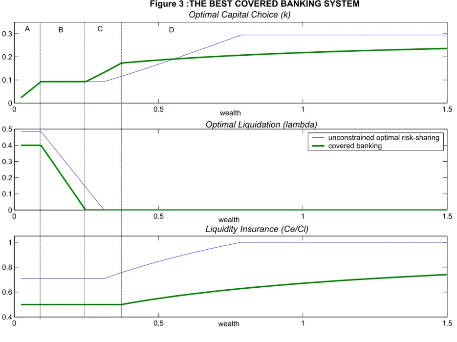
The General Shape of the Solutions.
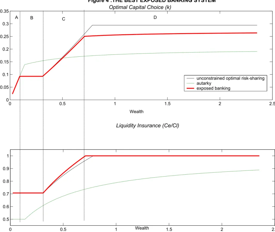
Before presenting thefirst best, covered and exposed contracts, it is possible to characterize the general shape of the solution. Technological considerations on the returns of the assets define four regions (A to D) depending on the level of wealth for the three solutions. Although the thresh-olds that define these regions differ among the three contracts, we define the generic thresholds: k, w˜j, and wˆj where j = {u, c, e} is an index for the unconstrained or first best solution, the covered banking and exposed banking solutions respectively.
regulation of banks.
21The two contracts are equivalent because in the absence of aggregate uncertainty the incentive compatibility
Region A: No investment in short-term technology, no liquidity provision.
For poor economies (w≤k) investing in capital dominates investing in the short asset because
the marginal return even is higher if it is liquidated. Therefore all wealth is invested in the long
technology (k = w), and early consumption is served by liquidating a constant proportion of this asset (λj is constant). Notice that the optimal portfolio is the same as under autarky. Since the
optimality of full investment in capital is a technological consideration, the optimal portfolio, and
the threshold of the region is common to all solutions.
Region B: Constant level of investment in capital, reduction of early liquidation, in-creasing liquidity provision.
For k≤ w ≤ wej the financial intermediary invests in both assets and provides extra liquidity. The defining characteristic of this region is that investment in capital is keptfixed atk. All optimal solutions keep the marginal return of the long asset fixed at a high level, where its value, when liquidated prematurely, equals the marginal return of storing the good.22 Even for a constant level
of the capital stock, output can grow because the bank is liquidating a decreasing proportion of the
long asset (λj is decreasing in wealth). The bank starts using the liquid asset as a source of liquidity
to pay out early consumers, reducing premature liquidation of the long asset. Late consumers are
served using an increasing proportion of the fully matured output.
Region C: No liquidation of long term investment, increasing investment in both assets.
When wealth has crossed a certain threshold (w ≥ wej), the financial intermediary stops using the long asset to serve early consumers. All the long technology is left until full maturity (λj = 0) to serve late consumers, and investment in capital can increase again. If there is no crisis, early
consumption is served only using the short asset (cjE = w−πkj), and late consumption using the long term technology (cjL = h1(−kjπ)). Increasing investment in capital over this region implies that the marginal return of the asset used to serve late consumers decreases relative to the return of the
asset used for early consumption.
Region D: No liquidation of long term investment, and excess liquidity.
For high levels of wealth (w >wˆj) high investment in capital has exhausted the marginal return of the long asset, and it is optimal to transfer some returns of storage to serve late consumers
(ij ≥0). Over this region there is no early liquidation of the long technology (λj = 0).
22Two assets can be used to serve the same type of consumption only if their marginal returns are the same at the
A general expression for early and late consumption for all contracts and all regions is given by:
cjE = w−k
j−ij +λjγh(kj)
π and c
j
L =
ij +¡1−λj¢h(kj) 1−π
We present first the main features of the efficient benchmark (4.1.2). Then we characterize the optimal covered (4.1.3), and exposed banking (4.1.4) contracts. Section (4.1.5) presents then the
optimal banking system as the bank’s choice between these contracts.
4.1.2 The Efficient Benchmark: Unconstrained Optimal Risk Sharing
Gaytan and Ranciere (2002) characterize the unconstrained optimal risk sharing solution. The main
implications for investment, liquidation policy and liquidity insurance are presented in the following
table:
w ku λu iu cE
cL
A 0< w ≤k w λ∗ 0 γσ1
B k≤w≤weu k λu
(w) 0 γσ1
C weu ≤w≤wˆu ku(w) 0 0 h0(ku)−1σ
D w≥wˆu k 0 (1−π) (w−k)−h(k) 1
where weu, wˆu, λ∗, λu(w) are de
fined by:23 :
e
wu =k
µ
1 + πγ
1/σ
(1−π)γβ
(17)
ˆ
wu =k
µ
1 + π
β(1−π) 
(18)
λ∗ = πγ
1
σ
πγ1σ + (1−π)γ
(19)
λu(w) =λ∗−(1−λ∗)βw−k
k (20)
Efficiency of the unconstrained solution can be summarized by the following conditions:
Technology efficiency:
23The definition of the unconstrained threholdsweu andwˆu is presented in the Appendix. ku(w)is a continuous,
strictly increasing and concave function implicitly defined by (see Gaytan and Ranciere (2002)):
u0(c E)
u0(cL) =h
(i) There is full investment in capital whenever the early liquidation marginal return on capital
exceeds the marginal return on storage (k =w ⇔ γh0(k)>1);
(ii) whenever there is liquidation of the long technology, capital investment never exceeds k (if
λ >0⇒ γh0(k)≥1);
(iii) when wealth is large enough (w≥wˆu) the bank fully exploits the marginal return on capital (k=k).
Liquidity efficiency:
(iv) There is never inefficient liquidation of the long technology (if γh0(k)≥1 ⇒ λ >0);
(v) whenever the marginal return of capital at maturity exceeds the marginal return on storage
there is no excess liquidity (if h0(k)>1 ⇒i= 0).
Efficient liquidity insurance:
(vi) Whenever there is early liquidation of the long asset (λ > 0), liquidity insurance is kept constant at a level that equates the marginal rate of substitution with the marginal return of
k (if λ >0⇒ u0(cE) u0(cL) =
1 γ);
(vii) wheneverγh0(k)<1, an increase in capital investment is optimally associated with an increase
in liquidity insurance;
(viii) excess liquidity is held (i > 0) only to make an efficient transfer from the early to the late subperiod to provide perfect insurance (ifi >0⇒ cE
cL = 1).
An important question is whether a bank that offers a contract that replicates the first best solution is vulnerable or not to panic runs. If the first best solution is run proof, it must be the optimal contract chosen both under covered, and under exposed banking; and therefore, it must
be the optimal banking solution. There is the following relationship between risk aversion and
invulnerability of thefirst best solution.
Proposition 4.1 (Optimal risk sharing and bank runs) (i) Ifσ >1(high risk aversion),
(ii) If σ≤1 (low risk aversion), there exists a unique level of wealth wrp∈(weu,wbu), such that:
— if w≤wrp, the unconstrained risk sharing solution is run proof (cE ≤cR)
— if w > wrp, the unconstrained risk sharing solution is vulnerable to crises (cE > cR).
wherewrp =krp(1 + (1−πγπ)βγσ) and h0 ¡
krp ¢
= γ1σ
Proof. See Gaytan and Ranciere (2002a).
Impatient agents (σ >1) have a stronger preference for liquidity insurance and demand higher early pay-off, making the first best contract vulnerable to runs. Patient agents (σ ≤ 1), on the other hand, prefer to enjoy higher payoffs on late withdrawals while the marginal returns are still high. However, as wealth increases and liquidity insurance improves, the economy reaches a point
where the optimal risk sharing solution becomes necessarily vulnerable to runs.24
For 0 < w ≤ wrp and σ ≤ 1, the first best solution is the optimal covered bank contract and the optimal banking solution. For higher levels of income, the optimal contracts are subject to the
optimality conditions that prevail for σ > 1. Therefore, we can concentrate our attention on the results for high risk aversion(σ >1).
4.1.3 Covered Banking (η= 0).
Before presenting the optimal covered contract, it is useful to notice that the autarkic solution is
run proof (ca
E = w−k+πγh(k) < w−k+γh(k)). A covered bank could always replicate the autarkic solution by settingλ=π, k =ka, andi= (1−π) (w−k)and, therefore, optimal covered banking will necessarily dominate the autarkic outcome.
Proposition 4.2 The optimal covered banking contract for high risk aversion (σ > 1) is charac-terized in the following conditions25:
24Improving insurance and the existence of a wealth level above which the economy is vulnerable to a run, represent
a difference with respect to the original DD model. In their original framework offixed returns to assets, low risk aversion (σ≤1) implied that the optimal risk sharing contract was necessarily run proof.
w u0(cE)
u0(cL) kc λ
c
ic
A 0< w ≤k γ1σ w π 0
B k≤w≤wec 1
γσ k λ
c(w) 0
C wec≤w≤wˆc 1
γσ kcC(w) 0 0
D w≥wˆc 1−π
π
[(11−−πγπ)h0(k)−1]
(1−γh0(k)) kDc (w) 0 (1−π) (w−kc)−πγh(kc) where the thresholds wec, wˆc, liquidation policy λu(w) , and investmentks(w)are given by:
e
wc = k
µ
1 + π
β(1−π) 
ˆ
wc = bkc
µ
1 + γπ
β(1−π)h
0³bkc´¶ W here:h0³bkc´= π+ (1−π)γσ
πγ+ (1−πγ)γσ
λc(w) =π−(1−π)βw−k
k (21)
kc(w) is implicitly defined by the marginal rate of substitution u0(cE)
u0(cL) and excess liquidity i
c.26
The source of distortions in covered banking is the limit imposed in the degree of liquidity
insurance. The unconstrained level of liquidity insurance violates the run preventive constraint,
therefore, a covered bank will provide a strictly lower level of liquidity than the first best. The incentive to increase early consumption towards the first best level, makes that the run preventive constraint binds for all levels of wealthcE =w−k+γh(k).This limit in early consumption forces the bank to provide a constant level of liquidity insurance over regions A, B and C (cE = γcL), below the efficient level. Lower liquidity insurance frees resources to provide higher late consumption either through reducing liquidation or increasing capital investment.
Over regions A and B, since capital is determined by pure technological considerations (k =w and k = k), a lower liquidity insurance implies a smaller liquidation of the long asset λc(w) < λu(w).27 The bank stops liquidating the long asset at lower levels of wealth (wec < weu). This reduction in liquidation increases the marginal product of capital and has a positive effect on economic growth. Once the covered economy has stopped early liquidation of the long technology
it starts increasing capital. However, over region C, the increase in capital is not accompanied by
an increase in liquidity insurance. Over region C and the first part of D, the bank ”over-invest”
26ks
in capital with respect to the first best level to maintain a covered contract. In the second part of region D, there is underinvestment in capital relatively to the first best, as ”excess liquidity” i >0becomes a more efficient way to restrict liquidity insurance. The use of excess liquidity before fully exhausting the return on the long asset (h0(k)< 1) is a technological inefficiency of covered
banking. Over region D, the bank can maintain a covered contract and increase liquidity insurance,
reducing the distortion generated by the run preventing constraint.
Making a banking system ”safe” implies restricting both the banks’ asset portfolio, and the
provision of liquidity insurance offered by the deposit contact in a way that banks can always satisfy any claim by depositors. In the previous literature, a requirement of excessive liquid reserves
can attain this objective. However, when returns are endogenous it is not necessarily the case. We
find that, except for rich economies, it is more efficient to reduce the promises to early consumers rather than to hold more liquid assets. This reduction of liquidity insurance allows the bank to
allocate more resources to long term projects, with positive consequences for economic growth.
4.1.4 Exposed Banking (η=q).
Proposition 4.3 The optimal exposed banking for high risk aversion (σ > 1) is characterized in the following conditions28
w u0(cE)
u0(cL) k
e λe ie
A 0< w ≤k 1
γ w λ∗ 0
B k≤w≤weu 1
γ =h0(k) k λ
u(w) 0
C weu ≤w≤wˆe h0(ke)− q
1−q(1−γh0(k
e))u0(cR)
u0(cL) k
e
C(w) 0 0
D w≥wˆe h0(ke)− q
1−q(1−γh0(k
e))u0(cR)
u0(cL) k
e
D(w) 0 (1−π) (w−ke)−πh(ke) Where wˆe is given by:
ˆ
we =bke 1 +
πh0³bke´
β(1−π)
where :h0³bke´= q+ (1−q) (π+ (1−π)γ) σ
γq+ (1−q) (π+ (1−π)γ)σ
ke
C(w) is implicitly defined by the expression for the marginal rate of substitution u0(cE)
u0(cL), and kc
Regions A and B of the exposed contract are identical to the intra-generationalfirst best solution. Since over these regions the level of investment is determined by technological efficiency, it is optimal to provide thefirst best level of liquidity insurance, because a reduction of liquidity insurance helps only if it makes the contract run proof (covered banking); otherwise, crises are still possible. As
a consequence, for this range of wealth an optimizing bank will be restricted to maximize utility
under the good state of no-crisis only.
Exposed banking introduces an important new element. Having crises with positive probability
generates aggregate uncertainty in the payoff for both types of consumers. The bank will have incentives to smooth consumption over realizations of the aggregate state. This ”banking
self-insurance” against crisis risk is done by increasing the payoffin the bad state, that is, by increasing the early liquidation value of the bank’s portfolio. Since the early value of the portfolio increases
with investment in the storage technology, the bank will invest less capital than the optimal risk
sharing over regions C and D.29
There is no conflict for the exposed bank between increasing liquidity insurance and increasing crises self-insurance. A promise of higher early consumption adds extra liquidity, which can be used
in case of afinancial crisis. That is why over region C the bank provides excessive liquidity insurance
³ce E ce
L > cu
E cu L
´
, and starts providing full liquidity insurance at a lower level of wealth (wˆe <wˆu). Excess liquidity (i > 0) is used to provide perfect insurance, although the marginal product of capital is not the same than that of storage. Since the marginal return on capital have not been
completely exhausted (h0(k) > 1), the bank will continue to increase capital as wealth increases
over D.30
Therefore a maximizing bank that faces a positive probability of a run, will increase the level
of liquidity and liquidity insurance beyond the first best solution increasing the vulnerability of
29In region C of the unconstrained problem, the marginal cost of increasing capital was justu0(c
E), the valuation
in terms of utility of the marginal return of storage. When crises occur with positive probability the marginal cost increases to
u0(c
E) + (1−γh0(k)) q
1−qu
0(c R)
because investment in capital also reduces consumption in case of a total run.
30It is interesting to notice that over region D (c
E =cL =c= w−k+h(k)), the optimality condition can be
written as:
region D: u
0(c R)
u0(c) =
(1−q) (h0(ke)−1)
q(1−γh0(ke))
the system and reducing the growth benefits. Although this ”excessive risk” result resembles those coming from a moral hazard problem, the distortion is not a consequence of insurance received, but
of insurance provided. In effect, by increasing liquidity the bank is providing crisis insurance. At the cost of lower returns, a more liquid system reduces the output loss in case of a crisis, because
it increases the bankruptcy value of the bank.
An exposed bank never ”over-invest”. At low levels of wealth (regions A and B), capital and growth are the same as under the unconstrained solution. For higher levels of wealth, the risk of a
run reduces the level of investment, with negative consequences for economic growth.
4.1.5 The Optimal Banking System
In this section we characterize the optimal risk sharing solution when there is an exogenous
probabil-ity of pessimism that can drive a panic run on the bank as the choice between the optimal”covered”
and ”exposed” contracts. For any given level of wealth, the financial intermediary will choose the contract that maximizes expected utility. The bank’s decision reflects the tension between crisis prevention and precautionary measures to minimize the costs of a possible crisis. The financial intermediary chooses η= arg max{V (η, w)}, whereV (η, w) =Max{Ve(q, w), Vc(w)}.
Since the distortions generated by the contracts vary with the level of wealth, the optimal
choice between the contracts will depend on wealth, and on the probabilty of a bad realization of
the sunspot. Expected utility of covered banking (Vc(w)) is invariant to q, while expected utility of the exposed contract (Ve(q, w)) is strictly decreasing inq. The choice between the two contracts will be determined by a wealth dependant cut-offprobability q∗(w). This threshold probability is
defined in the following proposition.
Proposition 4.4 The Optimal Banking System
For any level of wealth for σ > 1, and for w > wrp when σ ≤ 1, there exists a unique cut-off probability q∗ ∈(0, π] such that:
q > q∗(w)⇔a covered banking system is optimal
q < q∗(w)⇔an exposed banking system is optimal
whereq∗(w) is a continuous function defined by:
Proof. See Appendix A
Over region A and B the optimal exposed contract replicates the first best contract; therefore, there are no distortions in the contract, and the only cost is the expected cost of a run. This
cost increases with q and therefore expected utility is decreasing in q. Over regions C and D, a
positive probability of a runq increases the liquidation risk, reducing the expected marginal return
of capital, and investment.
Lower capital investment has two effects on expected utility: a positive effect because it increases liquidity insurance, and a negative effect because it reduces the returns for late consumption. The overall effect is negative, because the bank is increasing the expected payoffin case of a run at the cost of reducing it when there is no run, exacerbating the distortion in the non-run case.31 Over
regions C and D, every dollar kept for crisis self-insurance pays less in terms of utility than a dollar
invested to increase the payoffin the good equilibrium.
In Appendix B, we show that if the probability of the sunpot is higher than the probability of
the idiosyncratic liquidity shock (q > π), autarky dominates the exposed banking solution. Since
covered banking weakly dominates the autarkic outcome, the cutoff probability q∗(w) must be
strictly lower than π.
The cutoff probability determines the bank’s optimal choice of contract for any given level of wealth. However, it is useful to invert the problem andfind, for a given probability of the sunspot, how does the decision between the two contracts changes with the level of wealth? This analysis
sheds light over how the choice of the risk taken by an exposed bank varies over the development
path, or equivalently it provides a broad picture of the cross sectional distribution of risk for countries
with different levels of wealth.
Proposition 4.5 Optimal Banking and the Level of Wealth.
There exist two cutoff probabilities q0, q1 (0< q0 < q1 < π) such that:
(i) high probability of run: if q > q1, a covered banking system is the optimal for all levels of
wealth
31Using the envelope condition we can see that:
dVe(q, w)
(ii) intermediate probability of run: if q0 < q < q1, there exist two levels of wealth wl < wh such that an exposed banking system is optimal for middle income economies(wl< w < wh) and a covered banking system is optimal for poor and rich economies (w∈R+−[wl, wh])
(iii) low probability of run: if q < q0, there exist one level of wealth wh such that an exposed banking system is optimal, except for rich economies (w > wh)
where:
q0 =qo∗ =
·
π+(1−π)γσσ−1
¸σ
−[π+(1−π)γσ−1]
·
π+(1−π)γσ−σ1
¸σ
−1 q1 =Max{q∗(w)}< π
δwl δq >0;
δwh
δq <0 and limq→0wh = 0
Proof. See Appendix A
Figure 5 illustrates the characterization of the optimal solution in proposition 4.5. For any
probability of the pessimistic state (q in the horizontal axis), it shows the upper and lower wealth
0 0.05 0.1 0.15 0.2 0.25 0.5
1 1.5 2 2.5 3
3.5 Figure 5: The Optimal Banking System
Probability of Run (q)
Le
vel
o
f W
eal
th
Wlow Whigh
Case (iii) Case (ii)
Optimal: Exposed Banking
Optimal: Covered Banking
Optimal:Covered Banking
Optimal: Covered Banking
Case (i)
qzero qone
Optimal: Exposed Banking
For poor economies, the cost of covered banking is the low liquidity insurance provided by the
intermediary, however, the cost is partially compensated because lower liquidation increases late
consumption. On the other hand, since the exposed banking replicates the unconstrained solution,
the cost of exposed banking is the cost of a run. Therefore, poor economies will prefer a covered
contract when the probability of the pessimistic state is high enough (q > q0).
The underinsurance distortion of covered banking becomes more pervasive for higher levels of
wealth. Liquidity insurance is kept constant even when the return of the long asset is decreasing. In
addition, the covered bank eventually uses excessive liquidity (i > 0) to satisfy the run preventive constraint although the returns to the long assets are not fully exhausted (h0(k)>1).
On the other hand, an exposed contract does increase insurance and crisis insurance, partially
q that can make the exposed banking suboptimal.
There is always a high level of wealth after which covered banking is the optimal contract.
The distortions of covered banking tend to disappear as the bank increases liquidity insurance and
increases investment towards the best maximum capital (k); while the exposed banking always faces
an uninsurable crisis risk that prevents capital investment to achieve the maximum efficient level.32
Thee degree of exposure of the optimal banking system.
Even though under exposed banking crises happen with fixed probability, it is illustrative to construct an indicator of the degree of exposure of the banking system. Total runs are triggered when the proportion of late consumers that misrepresent their type is enough to violate the incentive
compatibility constraint. Therefore, we can define the maximum fraction of late consumers a bank can serve in the early sub-period without triggering a bank run33:
r= 1
(1−γ)(1−π) ·
cR
cE −
(π+ (1−π)γ) ¸
In this case (1−r) is a measure of the degree of exposure of the banking system.34 A covered contract that does not exhibit any exposure (1−r≤0) is run proof. This degree of exposure varies with the level of wealth. Since over regions A, B and CcR=πcE+γ(1−π)cL, we can express the degree of exposure as a function of liquidity insurance:
1−r = 1− γ 1−γ
" 1 cE cL
−1 #
for regions A,B and C
Exposed banking for low income economies (regions A and B) imply constant exposure. Over region
C, the increase in liquidity insurance leads to an increase in the degree of financial exposure. Over region D, ascE =cL=c, q−r can be expressed as:
1−r= 1
(1−γ)(1−π) h
1− cR c
i
for region D
Over region D, cR
c increases, and this increase in self-insurance against crises decreases the degree of financial exposure. In summary:
32In the limit for infinite large wealth kc attainsk, whileke attains an upperbound given by
h0(ke
max) =
1 qγ+ 1−q
33See Appendix * for details on the derivation ofr.
34An alternative interpretation of (1−r) is the minimum trust a bank needs to remain solvent. The more expose