The relevance of the EU banking sector to economic growth and the recent financial crisis

(1)

Cândida Ferreira

The relevance of the EU banking sector to economic

growth and the recent financial crisis

WP02/2015/DE/UECE _________________________________________________________

De pa rtme nt o f Ec o no mic s

W

ORKING

P

APERS

(2)

The relevance of the EU banking sector to economic growth and the recent financial crisis

Cândida Ferreira [1]

Abstract

Using static and dynamic panel estimates in a sample including all 28 European Union countries during the last decade, this paper seeks to improve upon the existing literature with empirical evidence on the important role that well-functioning EU banking institutions can play in promoting economic growth. The banking sector performance is proxied by the evolution of some relevant financial ratios and economic growth is represented by the annual Gross Domestic Product growth rate. In order to analyse the possible differences arising after the outbreak of the recent international financial crisis, the estimations consider two panels: one for the time period 1998– 2012 and another for the subinterval 2007–2012. The results obtained allow us to draw conclusions not only on the importance of the variation of different operational, capital, liquidity and assets quality financial ratios to economic growth but also on some differences evidenced in the two considered panels, reflecting the consequences of the recent financial crisis and the correspondent reactions of the European banking institutions.

Keywords: bank performance, economic growth, European Union, financial crisis, panel estimates JEL Classification: G21; F43; F36; C23.

___________________________________________________

[1]_{ISEG, UL – Lisboa School of Economics and Management of the University of Lisbon and UECE} - Research Unit on Complexity and Economics

Rua Miguel Lupi, 20, 1249-078 - LISBON, PORTUGAL tel: +351 21 392 58 00

(3)

The relevance of the EU banking sector to economic growth and the recent financial crisis

1. Introduction

During the last decade, and particularly after the outbreak of the recent international financial crisis, which deeply affected the European Union (EU) countries, concerns have mounted over the role of the financial institutions in dealing with the phenomena resulting from asymmetric information. It became more evident that the consequences of excessively risky credit supply can not only contribute to the possible collapse of some banking and other financial institutions, but also affect the process of financing the other economic sectors that contribute to economic growth. This paper seeks to improve upon the existing literature by testing the contribution of the EU banking institutions’ performance, proxied by some relevant financial ratios, to economic growth during the last decade and particularly after the recent financial crisis. Using static and dynamic panel estimation methods on a data set including all 28 current EU member states, we compare the results obtained for two panels: one considering the years between 1998 and 2012 and a second one for the subinterval spanning only from 2007 to 2012.

The results obtained reveal not only the importance of the variation of different operational, capital, liquidity and assets quality financial ratios to the Gross Domestic Product (GDP) growth rate but also some differences evidenced in the two considered panels, reflecting the consequences of the recent financial crisis and the European banking institutions’ reactions to the crisis.

(4)

2. Review of some relevant literature

The importance of the banking sector’s performance to economic growth has been the subject of intense theoretical debates and empirical studies, particularly after the publication of the renowned King and Levine papers (1993-a, 1993-b).

There is a strand of literature pointing to a general consensus that well-functioning banking institutions and financial markets contribute to economic growth by decreasing transaction costs and the problems connected to asymmetric information. Furthermore, banking institutions are supposed to facilitate trade and the diversification of risk, and also to increase the financial resources to assist economic growth, by mobilizing savings, identifying the best investment opportunities and selecting the most profitable projects.

Nevertheless, as already underlined by Khan and Senhadji (2000), while the general effects of financial development on the real outputs may be considered positive, the size of these effects varies not only with the different variables, namely with the chosen financial development indicators, but also with the estimation methods, data frequency or the defined functional forms of the relationships.

(5)

More recently, Greenwood et al. (2010, 2013) empirically analysed the effects of financial development on economic growth, deploying a state cost verification model, and concluded that as financial sector efficiency rises, financial resources get redirected from the less productive firms to their more productive peers. This analytical approach was applied to both U.S. and cross-country data (more precisely, to a 45-country sample, first applied in Beck et al., 2000) and one of the key findings points to the conclusion that world output could increase by 53 per cent if all countries adopted the best global financial practices.

Cecchetti and Kharroubi (2012) consider a sample of developed and emerging economies and study how financial development contributes to aggregate productivity growth and conclude in favour of an inverted U-shaped financial development effect, meaning that this development exerts a positive influence on productivity growth but only up to a certain point and after that point the influence on growth turns negative. Moreover, these authors focus also on advanced economies, showing that a fast-growing financial sector can be detrimental to aggregate productivity growth. Other studies had already underlined that the contribution of the financial intermediaries to economic growth is far from consensual as the financial institutions can also be subject to adverse selection and moral hazard problems that will constrain real economic growth through non-adequate resource allocation, exaggerating the fluctuations in interest rates, or contributing to the decrease of the prevailing saving rates (among others, Bhide, 1993; Bencivenga et al., 1995; Rajan and Zingales, 1998; Shan, 2005).

(6)

bank deposits are negatively associated with economic growth; however, on the stock market side, their results indicate that stock market size and liquidity do contribute to growth.

There is also another strand of literature testing the causality relations between financial development and economic growth, including authors such as Berthelemy and Varoudakis (1996) and Greenwood and Bruce (1997), who believe that there may be a reverse causality between economic growth and financial development; others (like Demetriades and Hussein, 1996; Shan et al., 2001; Calderon and Liu, 2003; Bangake and Eggoh, 2011; Kar et al., 2011; Abdelhafidh, 2013) assume that there is a two-way causality relationship between financial development and economic growth.

Hassan et al. (2011) analyse how financial development links to economic growth applying Granger causality tests for a sample period between 1980 and 2007, and categorizing low- and middle-income countries into six geographic regions: East Asia and the Pacific, Europe and Central Asia, Latin America and the Caribbean, Middle East and North Africa, South Asia and Sub-Saharan Africa; and also two groups of high-income countries: OECD and non-OECD countries. The conclusion to be drawn from their finding is that the evidence favours the contribution of financial development to economic growth, particularly in low- and middle-income countries.

(7)

role of credit market frictions in the performance of the real economic activity during the recent crisis, using a sample including a large cross section of firms from 50 countries in both advanced and emerging market economies.

To our knowledge, not many studies have empirically tested the relevance of the banking sector’s performance to economic growth in the context of all the European Union member states.

In Ferreira (2008), quarterly data were used to analyse the possible influence of the financial systems on economic growth, in the context of the integration of new member states in the European Union. The real per-capita GDP growth was explained by the following variables: the real growth of domestic credit, the foreign liabilities, the sum of the bonds and money market instruments, the bank assets/bank liabilities ratio, and the domestic credit/bank deposits ratio. Two balanced panels were considered with subsets of EU countries: one including 11 “old” EU member countries (excluding Luxembourg, Denmark, Ireland and Sweden) for the period between Q2 1980 and Q4 1998, and another including 24 EU countries (excluding only Luxembourg) for the period between Q2 1999 and Q4 2002. The results obtained confirm the importance of the included financial variables to the real per-capita GDP growth and also the relatively more homogeneous behaviour in the panel considering only 11 of the “old” member states.

Koetter and Wedow (2010) analysed the relevance of banking financial intermediation to economic growth but in 97 German economic planning regions for the time period between 1993 and 2004 and concluded that the quality of these banks, defined by bank cost efficiency, robustly contributes to growth, while the quantity of bank credit provided does not clearly correlate with

economic growth. The same kind of conclusions were also obtained by Hasan et al. (2009), who

studied whether regional growth in 11 European countries was influenced by bank costs and profit

efficiency over the time period 1996–2005. Their findings indicate how, in these countries, an

increase in bank efficiency generates five times more influence on economic growth than the same

(8)

Recently, Ferreira (2015) also analysed the effects of the performance of the banking institutions on GDP growth using panel estimations and considering 27 EU countries for the time period between 1996 and 2008. Bank performance is represented not only by the traditional ROA and ROE ratios but also by bank efficiency, measured through Data Envelopment Analysis (DEA) and taking into account the influence of bank market concentration represented by the percentage share of the total assets held by the three largest banking institutions (C3). The main findings point to the expected and statistically significant positive influence of the ROA and ROE ratios and also of the DEA bank cost efficiency, and, although less strongly, to a negative effect of the C3 bank market concentration measure on EU economic growth.

3. Data and estimation methodology

3.1. Data

In our estimations we use data sourced from the European Commission database, AMECO, more precisely the dependent variable, GDP and also the financial sector leverage, that is, the ratio of debt to equity. All the other financial ratios are sourced from the privately owned financial database maintained by the Bureau van Dijk, BankScope.

Taking into account the classifications and definitions proposed by the BankScope database we consider the banking sector (more precisely, all commercial and savings banks) of each of the 28 current EU member states and opt to use different kinds of financial ratios, more precisely:

Operational ratios:

(9)

lending operations of the bank. The increase of the margins is usually considered as desirable but only as long as the asset quality is being maintained.

- Return on Average Assets, which is the ratio of the net income to the total assets of the banks and is useful in the assessment of the use of the banks’ resources and their financial strength. This ratio is often considered to be the most important single ratio in comparing the efficiency and operational performance of banks as it takes into account the returns generated from the assets financed by the bank.

- Cost to Income, which is one of the most cited ratios as it measures the overheads or costs of operating the bank as the percentage of income generated before provisions. It is a useful measure of bank efficiency, although it can be distorted by high net income from associates or volatile trading income; moreover, if the lending margins in a particular country are comparatively very high then the cost-to-income ratio will improve as a result of this situation.

Capital ratios:

- Equity to Total Assets, which is one of the most important capital ratios, representing the book value of equity divided by the total assets. Taking into account that equity represents a cushion against asset malfunction, the equity-to-total-assets ratio measures the amount of protection afforded to the bank by the equity invested in the bank; the higher this ratio is, the more protected the bank is. Furthermore, this ratio measures the bank leverage levels and reflects the differences in risk preferences across banks.

- Debt to Equity, which also measures the leverage levels and particularly the solvency of the bank, as this ratio represents the percentage of the bank’s equity that is owed by its creditors. It is a useful measure to evaluate the amount of risk that the bank creditors will be taking on by providing financial support to the bank.

(10)

Liquidity ratios:

- Net Loans to Total AssetsRatio, which is a liquidity measure and also a credit risk measure, obtained through the percentage of the assets of the bank that is tied up in loans; the lower this ratio is, the more liquid the bank will be.

- Net Loans to Total Deposits and Borrowings, which is also a measure of bank liquidity, similar to the previous one, but its denominator includes the bank deposits and borrowings with the exception of capital instruments.

Assets quality ratio:

- Impaired Loans to Gross Loans, which is a measure of the amount of the total loans that is doubtful, representing the quality of the bank assets; the lower this ratio is, the better the bank asset quality is.

Different combinations of these ratios were included in the four estimated models in order to explain their influence on economic growth, here represented by the Gross Domestic Product, more precisely, the AMECO series “GDP total in national currency (including ‘euro fixed’ series for euro area countries), current prices – annual data”.

We aim to analyse the bank performance contribution to the GDP growth (the natural logarithm of the GDP) of all the current EU member states as well as the possible differences after the outbreak of the recent financial crisis considering two panels of EU countries: one for the time period 1998–2012 and another for the shorter interval 2007–2012.

(11)

The Levin, Lin and Chu (2002) may be viewed as a pooled Dickey-Fuller test, or as an augmented Dickey-Fuller test, including lags and the null hypothesis stems from the existence of non-stationarity. This test is adequate for heterogeneous panels of moderate size, such as the panels included in this paper. The results, considering the first differences of the chosen series, are reported in Appendix A and enable us to reject the existence of the null hypothesis.

3.2. Estimation methodology

The use of a panel data approach in our estimations not only guarantees more observations for estimations, but also reduces the possibility of multicollinearity among the different variables. Following, among others, Wooldridge (2010), we consider the general multiple linear panel regression model for the cross unit (in our case, the country’s i bank sector, defined as the sample of all commercial and saving banks) i = 1,…,N, which is observed for several time periods t =1,…,T:

t i i t i t

i x c

y_,   '_,   _,

where: yi,tis the dependent variable (that is, each country’s i GDP growth rate at time t);



is the

intercept; xi,tis a K-dimensional row vector of explanatory variables (here, the presented bank

sector financial ratios) excluding the constant;



is a K-dimensional column vector of parameters; ci is the individual country-specific effect; and



,tis an idiosyncratic error term.

As we are dealing with balanced panels, we guarantee that each individual, i (here each country’s banking sector), is observed in all time periods, t. And one of the main advantages of using a panel data approach in this kind of cross-country regression is its ability to deal with the time-invariant individual effects (ci).

(12)

explanatory variables. In order to decide either to use fixed- or random-effects estimates it is possible to implement the Hausman (1978) procedure, which tests the null hypothesis that the conditional mean of the disturbance residuals is zero. The fixed-effects model will be preferred over the random-effects one if the null hypothesis is rejected; in contrast, the random-effects approach will be more appropriate than the fixed-effects method if the null hypothesis is accepted. However, neither fixed- nor random-effects models can deal with endogenous regressors, which may reveal an important concern in the context of the considered model. In order to deal with this limitation, we use dynamic panel estimates, developed by Arellano and Bover (1995) and Blundell and Bond (1998), which can not only address the endogeneity problems (although only for weak endogeneity and not for full endogeneity, as explained by Bond (2002)) but also reduce the potential bias in the estimated coefficients.

Here we chose the robust one-step and two-step system GMM (Generalized Method of Moments) estimates. The system GMM method uses cross-country information and jointly estimates the equations in first difference and in levels, with first differences instrumented by lagged levels of the dependent and independent variables and levels instrumented by first differences of the regressors.

(13)

In order to avoid the problems connected to the proliferation of instruments in relatively small samples, like the one we are using here, Roodman (2009) says that in these kinds of estimations the number of instruments should not approach or exceed the number of cross units (in our case, the number of EU countries).

4. Empirical results

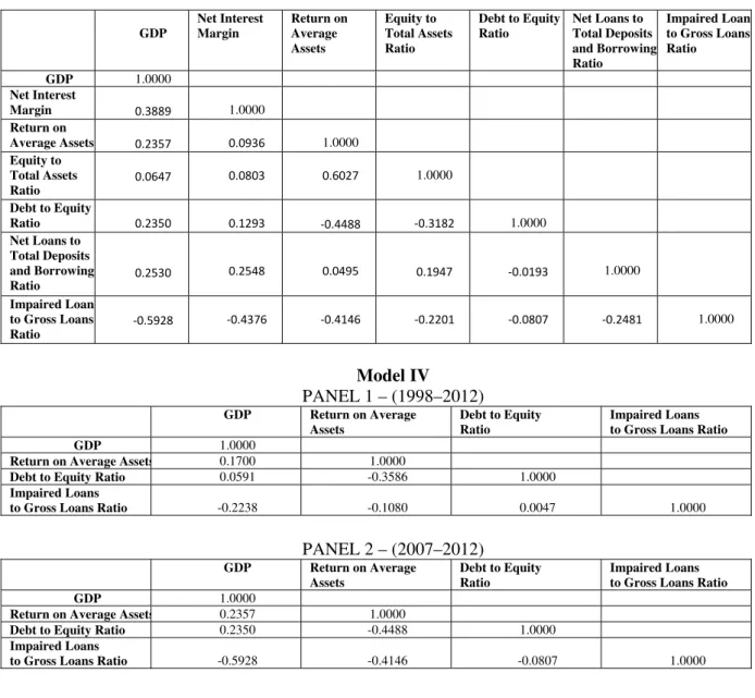
Using different combinations of the presented financial ratios as instruments, we estimate four models, considering for each of them two time periods: a longer one, between 1998 and 2012 (Panel 1), and another one, for the interval spanning only from 2007 to 2013 (Panel 2), as we want to analyse the possible differences after the outbreak of the recent financial crisis. Appendix B reports the correlation matrices of these models.

We will analyse the results obtained for the considered four models with robust panel random-effects estimates and also with robust dynamic panel-data one-step and two-step system GMM estimates. As the coefficients obtained with the used panel estimation methodologies are very stable across the different model specifications, we will comment on their economic meaning once for all.

We opt to present the results obtained with panel robust random-effects estimates, assuming that the unobserved variables are uncorrelated with the observed ones, as these results are completely in line with those obtained with robust fixed-effects estimates and the Hausman test did not clearly validate the fixed-effects approach.

Table 1 around here

(14)

values allow us to conclude that our estimates are in general robust, meaning that the evolution (first differences) of the chosen financial ratios is statistically relevant to explain the GDP growth rate (first differences of natural logarithms). This relevance is also corroborated in Panel 1 (1998– 2012) as the results obtained for all financial ratios included in each of the four models are statistically very robust.

In order to test the robustness of the results obtained with random-effects estimates we use robust dynamic panel-data system GMM estimates that reduce the potential bias in the estimated coefficients and control for the potential endogeneity of all explanatory variables.

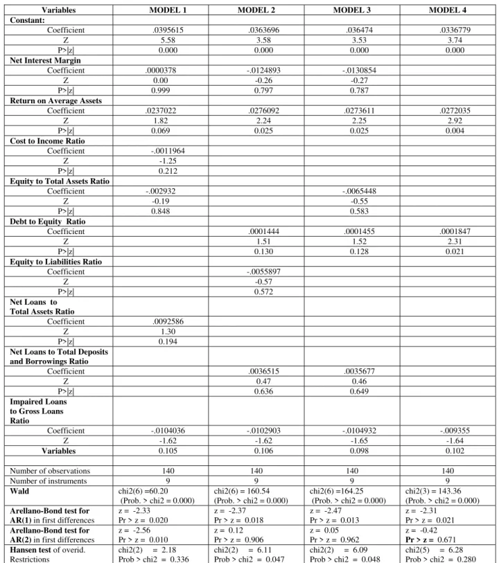
Here we begin by using the robust one-step estimates of the standard errors, which are consistent in the presence of any pattern of heteroskedasticity and autocorrelation within panels, and we present the results obtained in Table 2.

In both panels, and more clearly in Panel 1, the Wald tests results reveal the overall fit of the considered models. The Roodman (2009) rule of thumb is respected in all estimations as in the models of Panel 1 the number of instruments is 27 and in the models of Panel 2 the number of instruments is 9, thereby never exceeding the current number of the EU countries.

The quality of these one-step estimates in Panel 1 is corroborated by the results obtained, in the four models, with the Arellano and Bond (1991) tests as they clearly reject the null hypothesis of no autocorrelation of the first order and do not reject the hypothesis of no autocorrelation of the second order. Moreover, the Hansen J statistic does not reject the overidentifying restrictions, allowing us to believe that all included instruments are valid.

(15)

no autocorrelation of the second order. At the same time, the Hansen J statistic validates all the internal and external instruments in models 1 and 4 but not so clearly in the other two models. In our estimations we also used the robust dynamic system GMM two-step estimates of the standard errors, which are considered asymptotically more efficient than the one-step estimates. However, as demonstrated by Arellano and Bond (1991) and by Blundell and Bond (1998), in a finite sample the standard errors reported with two-step estimates tend to be severely downward biased. In order to compensate this bias, Windmeijer (2005) recommends a finite-sample correction to the two-step covariance matrix, which could make the two-step estimates more efficient than the one-step ones, but unfortunately, here, the limited number of current EU countries (our cross-section units) did not allow us to apply the Windmeijer correction.

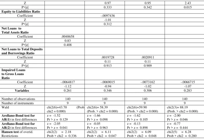
Nevertheless, the results obtained using robust dynamic two-step system GMM estimates, presented in Table 3, are completely in line with those obtained with the one-step estimates. In both panels and for the considered models, the Wald test results validate the estimations. As before, for Panel 1 (1998-–2012), in all models the Hansen test clearly does not reject the null that the instruments are valid and that they are not correlated with the errors, and, according to the results reported for the Arellano-Bond tests, the validity of the instruments is clearly supported as the residuals are always AR (1), but not AR (2).

(16)

The results obtained for the considered models with the used panel estimation methodologies are summarized in Table 4 and clearly show that, although not always with the same statistical robustness, the coefficients are always very stable across the different model specifications and estimation methodologies.

With regard to Panel 1, as expected, the evolution of the Return on Average Assets (included as an instrument in the four considered models) always goes in line with the GDP growth rate, revealing that the increase in efficiency and operational performance of the banking sector will contribute to the economic growth of the EU member states.

Staying with the results reported in Table 4 for Panel 1, we can look at two other financial ratios that clearly go in line with the GDP growth rate, namely the Equity-to-Total-Assets ratio, indicating that more protected banks will be relevant to economic growth, and the Debt-to-Equity ratio, revealing that during this time period the bank sector leverage levels and the correspondent risks may have increased but they did not contradict economic growth. The Equity-to-Liabilities ratio, which is another bank leverage ratio, as well as the Net-Loans-to-Total-Assets and Net-Loans-to-Total-Deposits-and-Borrowings ratios also grow in line with GDP.

Not surprisingly, the evolution of the Impaired-Loans-to-Gross-Loans ratio, representing the dubious provided bank loans, is negatively related to the GDP growth rate; and the same occurs with the Cost-to-Income ratio as the increase of the banking operational costs may be synonymous with less efficiency in providing the necessary bank financing of productive investments that will contribute to economic growth.

(17)

a more attentive look at the evolution of the bank Net Interest Margins reveals that during the considered time period they were in many cases decreasing, so it is not a real surprise to find that their evolution was not in line with economic growth.

Most of these tendencies were kept after the outbreak of the recent financial crisis, as evidenced by the results still reported in Table 4 but for the years between 2007 and 2012 (Panel 2). Nevertheless, there are also some differences, due to the reactions of European banking to the financial crisis. More precisely, during this shorter time period the evolution of the Equity-to-Liabilities and Equity-to-Total-Assets ratios was opposite to the GDP growth rate, as a symptom of the decrease of the bank sector leverage levels after the outbreak of the crisis. At the same time, and revealing the tendency to the increase of the traditional bank activities that was another response to the crisis, in Panel 2 the evolution of Net Interest Margins is now in line with the economic growth.

5. Summary and conclusions

Using static and dynamic panel estimates in a sample of all 28 EU member states during the last decade this paper provides empirical evidence of the important role that well-functioning banking institutions can play in promoting economic growth, here represented by the annual GDP growth rate. The data were sourced from the AMECO database and mostly from the Bankscope database as the performance of the banking institutions was proxied by some relevant financial ratios, including operational, capital, liquidity and assets quality ratios. In order to analyse the possible differences arising after the outbreak of the recent international financial crisis, the estimations considered two panels: one for the time period 1998–2012 and another for the subinterval 2007-– 2012.

(18)

1. With regard to the included operational ratios:

 For the first panel (1998–2012) there is clear and statistically strong evidence that the variation (mostly the decrease) of the Net Interest Margins, representing the traditional borrowing and lending operations, contrasts he GDP growth rate; but after the outbreak of the crisis (2007–2012) this variation is in line with economic growth, confirming that after the crisis many banking institutions decided to give emphasis to the traditional banking activities.

 In both panels there is clear evidence that the variation of the Return on Average Assets of the EU banking institutions contributes positively to economic growth.

 And although not with the same statistical strength, there is still evidence that before and after the crisis, the increase of the Cost-to-Income ratio, a proxy for less bank efficiency, does not contribute to the GDP growth rate.

2. With regard to the capital ratios:

 The contribution to economic growth of the Equity-to-Total-Assets ratio, one of the measures of the banking leverage levels and the correspondent risk preferences, also reveals the differences in the behaviour before and after the outbreak of the international crisis. In our first panel (1998–2012) this ratio increases in line with the GDP, but for the subinterval 2007-2012 it looks like it is opposite to the economic growth as a symptom of the decrease of the banking leverage levels.

 There is clear evidence that in both panels, the increase of the bank solvency, here represented by the evolution of the Debt-to-Equity ratio, contributes positively to the GDP growth rate.

(19)

but it is in contrast to the GDP growth in the subinterval 2007–2012, confirming the tendency to increase the bank protection after the outbreak of the crisis.

3. As for the liquidity ratios:

 There is clear evidence that in both panels more liquid banks, here represented by the Net-Loans-to-Total-Assets ratio, contribute positively to the GDP growth rate.

 The same results were obtained when bank liquidity was proxied by the Net-Loans-to-Total-Deposits-and-Borrowings ratio.

4. Finally, for the assets-quality ratio:

 As expected, the increase of the Impaired-Loans-to-Gross-Loans ratio, representing the fall of the quality of the bank assets, clearly contradicts the GDP growth rate, before and after the recent international financial crisis.

These results lead us to conclude that, although banking institutions were generally considered responsible for the recent financial crisis, their wealthy performance could also be a relevant contribution to economic growth, at least in the universe of all 28 EU member states during the last decade.

References

Abdelhafidh, S. (2013) “Potential financing sources of investment and economic growth in North African countries: A causality analysis”, Journal of Policy Modelling, 35, pp. 150–169.

Arellano, M. and S Bond (1991) “Some tests of specification for panel data: Monte Carlo evidence and an application to employment equations”, The Review of Economic Studies, 58, pp. 277–297.

Arellano, M. and O. Bover (1995) “Another look at the instrumental-variable estimation of error-components model”, Journal of Econometrics, 68, pp. 29–52.

(20)

Bangake, C. and J. Eggoh (2011) “Further evidence on finance-growth causality: A panel data analysis”,

Economic Systems, 35, pp. 176–188.

Beck, T., A. Demirgüç-Kunt and R. Levine (2000) “A new database on financial development and structure”, World Bank Economic Review, 14, pp. 597–605.

Beck, T., A. Demirgüç-Kunt and R. Levine (2004) Finance, Inequality and Poverty: Cross-Country Evidence, World Bank Policy Research Working Paper No. 3338.

Bencivenga, V., B. Smith and R. Starr (1995) “Transaction costs, technological choice and endogenous growth”, Journal of Economic Theory, 67, pp. 53–117.

Berthelemy, J.C. and A.Varoudakis (1996) “Economic growth, convergence clubs, and the role of financial development”, Oxford Economic Papers, 48, pp. 300–328.

Bhide, A. (1993) “The hidden costs of stock market liquidity”, Journal of Financial Economics, 34, pp. 1–51.

Blundell, R. and S. Bond (1998) “Initial conditions and moment restrictions in dynamic panel data models”, Journal of Econometrics, 87, pp.115–143.

Bond, S. (2002), Dynamic Panel Data Models: A Guide to Micro Data Methods and Practice, Institute forFiscal Studies, London, Working Paper No. 09/02.

Calderon, C. and L. Liu (2003) “The direction of causality between financial development and economic growth”, Journal of Development Economics, 72, pp. 321–334.

Cecchetti, S. and E. Kharroubi (2012) Reassessing the Impact of Finance on Growth, Bank for International Settlements, Working Paper No. 381.

Dell’Ariccia, G., E. Detragiache and R. Rajan (2008) “The real effect of banking crises”, Journal of Financial Intermediation, 17(1), pp. 89–112.

Demetriades, P. and K. Hussein (1996) “Does financial development cause economic growth? Time series evidence from 16 countries”, Journal of Development Economics, 5, pp. 387–411.

Demirguç-Kunt, A. and R. Levine (1999) Bank-Based and Market-Based Financial Systems: Cross Country Comparisons, World Bank Policy Research Working Paper, No 2143.

Ferreira, C. (2008) “The banking sector, economic growth and European integration”, Journal of Economic Studies, 35 (6), pp. 512–527.

Ferreira, C. (2015) “Does bank performance contribute to economic growth in the European Union?”,

Comparative Economic Studies, forthcoming.

Gaytan, A. and R. Rancière (2004) Wealth, Financial Intermediation and Growth, Departments of Economics and Business, Universitat Pompeu Fabra, Economics Working Papers No 851.

Greenwood, J. and S. Bruce (1997) “Financial markets in development, and the development of financial markets”, Journal of Political Economy, 98, pp. 1076–1107.

Greenwood, J., C. Wang and J. M. Sanchez (2010) “Financing development: The role of information costs”, American Economic Review, 100, pp. 1875–1891.

Greenwood, J., J.M. Sanchez and C. Wang (2013) “Quantifying the impact of financial development on economic development”, Review of Economic Dynamics, 16, pp. 194–215.

Hasan, I., M. Koetter and M. Wedow (2009) “Regional growth and finance in Europe: Is there a quality effect of bank efficiency?”, Journal of Banking and Finance, 33, pp. 1446–1453.

Hassan, M., B. Sanchez, and J. Yu. (2011) “Financial development and economic growth: New evidence from panel data”, The Quarterly Review of Economics and Finance, 51, pp. 88–104.

(21)

Kaminsky, G. L. and C. Reinhart (1999) “The twin crises: The causes of banking and balance-of-payments problems”, American Economic Review, 89 (3), pp. 473–500.

Kar, M., S. Nazlioglu and H. Agir (2011) “Financial development and economic growth nexus in the MENA countries: Bootstrap panel granger causality analysis”, Economic Modelling, 28, pp. 685–693.

Khan, M. S. and A. Senhadji (2000) Financial Development and Economic Growth: An Overview, IMF Working Paper No 209.

King, R. and R. Levine (1993-a) “Finance and growth: Schumpeter might be right”, Quarterly Journal of Economics, 108, pp. 717–737.

King, R. and R. Levine (1993-b) “Finance, entrepreneurship and growth: Theory and evidence”, Journal of Monetary Economics, 32, pp. 513–542.

Koetter, M. and M. Wedow (2010) “Finance and growth in a bank-based economy: Is it quantity or quality that matters?” Journal of International Money and Finance, 29, pp. 1529–1545.

Laeven, L. and F. Valencia, F. (2013) “The Real Effects of Financial Sector Interventions during Crises",

Journal of Money, Credit and Banking, 45(1), pp. 147-177.

Laeven, L., D. Klingebiel and R. Krozner (2002) Financial Crises, Financial Dependence, and Industry Growth, World Bank Research Working Paper No. 2855.

Levin, A, C. Lin and C. Chu (2002) “Unit Root Tests in Panel Data: Asymptotic and Finite Sample Properties”, Journal of Econometrics, 108, pp. 1–24.

Levine, R. and S. Zervos (1998) “Stock markets, banks and economic growth”, American Economic Review, 88 (3), pp. 537–558.

Loayza, N. V. and R. Rancière (2006) “Financial development, financial fragility, and growth”, Journal of Money, Credit and Banking, 38(4), pp. 1051–1076.

Rajan, R. and L. Zingales (1998) “Financial dependence and growth”, AmericanEconomic Review, 88, pp.559–587.

Roodman, D. (2009) “A note on the theme of too many instruments”, Oxford Bulletin of Economics and Statistics, 71(1), pp. 135–158.

Shan, J. (2005) “Does financial development ‘lead’ economic growth? A vector auto-regression appraisal”, Applied Economics, 37, pp. 1353–1367.

Shan, J., A. Morris, A. and F. Sun (2001) “Financial development and economic growth: An egg– chicken problem?” Review of International Economics, 9, pp. 443–454.

Windmeijer, F. (2005) “A finite sample correction for the variance of linear efficient two-step GMM estimators”, Journal of Econometrics, 126, pp. 25–51.

Wooldridge, J. M. (2010) Econometric Analysis of Cross Section and Panel Data, the MIT Press.

APPENDIX A – PANEL UNIT ROOT TEST

PANEL 1 – (1998–2012)

Variables Coefficient t-star P > t obs.

GDP -0.45558 -5.56807 0.0000 351

Net Interest Margin -1.08930 -19.31776 0.0000 351

Return on Average Assets -1.11523 -23.67703 0.0000 351

Cost to Income Ratio -1.43582 -28.31398 0.0000 351

Equity to Total Assets Ratio -1.27586 -22.14069 0.0000 351

Debt to Equity Ratio -1.13918 -15.61671 0.0000 351

Equity to Liabilities Ratio -1.46836 -28.22642 0.0000 351

(22)

Net Loans to Total Deposits

and Borrowings Ratio -1.05457 -16.26953 0.0000 351

Impaired Loans to

Gross Loans Ratio -0.98484 -16.44459 0.0000 351

PANEL 2 – (2007ü2012)

Variables Coefficient t-star P > t obs.

GDP -1.14952 -21.08455 0.0000 108

Net Interest Margin -1.29413 -10.66102 0.0000 108

Return on Average Assets -1.31640 -8.78615 0.0000 108

Cost to Income Ratio -1.45812 -46.31647 0.0000 108

Equity to Total Assets Ratio -1.18626 -12.72064 0.0000 108

Debt to Equity Ratio -1.48950 -14.40565 0.0000 108

Equity to Liabilities Ratio -0.59464 -5.28540 0.0000 108

Net Loans to Total Assets Ratio -1.30110 -18.89312 0.0000 108

and Borrowings Ratio -1.37850 -21.48547 0.0000 108

Impaired Loans to

Gross Loans Ratio -1.28129 -12.44569 0.0000 108

APPENDIX B – CORRELATION MATRICES

MODEL I

PANEL 1 – (1998–2012)

GDP Net Interest Margin Return on Average Assets Cost to Income Ratio Equity to Total Assets Ratio

Net Loans to Total Assets Ratio

Impaired Loan to Gross Loans Ratio

GDP 1.0000

Net Interest

Margin -0.2095 1.0000

Return on Avera

Assets 0.1700 0.0089 1.0000

Cost to Income

Ratio -0.0346 -0.1465 0.1387 1.0000

Equity to Total Assets Ratio

-0.0007 0.2166 0.0170 -0.0116 1.0000

0.1657 0.1370 -0.0026 -0.0348 -0.1958 1.0000

Impaired Loans to Gross Loans Ratio

-0.2238 -0.0997 -0.1080 -0.0246 0.0150 -0.0357 1.0000

PANEL 2 – (2007–2012)

GDP Net Interest Margin Return on Average Assets Cost to Income Ratio Equity to Total Assets Ratio

GDP 1.0000

Net Interest

Margin 0.3889 1.0000

Return on

Average Assets 0.2357 0.0936 1.0000

Cost to Income

Ratio -0.0630 -0.1802 0.2992 1.0000

Equity to Total

Assets Ratio 0.0647 0.0803 0.6027 0.3199 1.0000

0.2638 0.2413 -0.1153 -0.0022 -0.0897 1.0000

-0.5928 -0.4376 -0.4146 0.0199 -0.2201 -0.1809 1.0000

Model II

(23)

GDP

Net Interest Margin

Return on Average Assets

Debt to Equity Ratio

Equity to Liabilities Ratio

Net Loans to Total Deposits and Borrowing Ratio

GDP 1.0000

Net Interest

Margin -0.2095 1.0000

Return on

Average Assets 0.1700 0.0089 1.0000

Debt to Equity

Ratio 0.0591 0.0328 -0.3586 1.0000

0.0085 0.2030 -0.0684 0.0010 1.0000

0.1296 0.1689 0.0554 0.0058 -0.1800 1.0000

-0.2238 -0.0997 -0.1080 0.0047 0.0028 -0.0315 1.0000

PANEL 2 – (2007–2012)

GDP

GDP 1.0000

Net Interest

Margin 0.3889 1.0000

Return on

Average Assets 0.2357 0.0936 1.0000

Debt to Equity

Ratio 0.2350 0.1293 -0.4488 1.0000

0.0664 0.0834 0.6011 -0.3418 1.0000

0.2530 0.2548 0.0495 -0.0193 0.1969 1.0000

-0.5928 -0.4376 -0.4146 -0.0807 -0.2132 -0.2481 1.0000

Model III

PANEL 1 – (1998–2012)

GDP Net Interest Margin Return on Average Assets Equity to Total Assets Ratio

GDP 1.0000

Net Interest

Margin -0.2095 1.0000

Return on

Average Assets 0.1700 0.0089 1.0000

-0.0007 0.2166 0.0170 1.0000

Debt to Equity

Ratio 0.0591 0.0328 -0.3586 -0.0435 1.0000

0.1296 0.1689 0.0554 -0.1281 0.0058 1.0000

-0.2238 -0.0997 -0.1080 0.0150 0.0047 -0.0315 1.0000

(24)

GDP Net Interest Margin Return on Average Assets Equity to Total Assets Ratio

GDP 1.0000

0.3889 1.0000

0.2357 0.0936 1.0000

0.0647 0.0803 0.6027 1.0000

Debt to Equity

Ratio 0.2350 0.1293 _‐0.4488 ‐0.3182 1.0000

Net Loans to Total Deposits and Borrowing Ratio 0.2530 0.2548 0.0495 0.1947

‐0.0193 1.0000

‐0.5928

‐0.4376 ‐0.4146 ‐0.2201 ‐0.0807 ‐0.2481 1.0000

Model IV

PANEL 1 – (1998–2012)

GDP Return on Average Assets

Impaired Loans to Gross Loans Ratio

GDP 1.0000

Return on Average Assets 0.1700 1.0000

Debt to Equity Ratio 0.0591 -0.3586 1.0000

Impaired Loans

to Gross Loans Ratio -0.2238 -0.1080 0.0047 1.0000

PANEL 2 – (2007–2012)

GDP Return on Average Assets

GDP 1.0000

Return on Average Assets 0.2357 1.0000

Debt to Equity Ratio 0.2350 -0.4488 1.0000

Impaired Loans

to Gross Loans Ratio -0.5928 -0.4146 -0.0807 1.0000

TABLE 1 – RESULTS OBTAINED WITH ROBUST PANEL RANDOM-EFFECTS ESTIMATES

PANEL 1 – (1998–2012)

Variables MODEL 1 MODEL 2 MODEL 3 MODEL 4 Constant:

Coefficient .0522928 .052782 .0528509 .0570513

Z 11.89 11.30 11.24 8.73

P>|z| 0.000 0.000 0.000 0.000

Net Interest Margin

Coefficient -.020414 -.0197993 -.0194422

Z - 2.73 -2.58 -2.52

P>|z| 0.006 0.010 0.012

Return on Average Assets

Coefficient .0077313 .009462 .0090373 .0088976

Z 1.92 2.41 2.33 2.07

P>|z| 0.054 0.016 0.020 0.038

Cost to Income Ratio

Coefficient -.0001108

Z -2.59

P>|z| 0.010

Equity to Total Assets Ratio

Coefficient .0011713 .0009857

Z 2.94 2.11

P>|z| 0.003 0.035

Debt to Equity Ratio

(25)

Equity to Liabilities Ratio

Coefficient .0001745

Z 3.25

P>|z| 0.001

Net Loans to Total Assets Ratio

Z 3.15

P>|z| 0.002

Net Loans to Total Deposits and Borrowings Ratio

Coefficient .0017024 .0016124

Z 2.82 2.79

P>|z| 0.005 0.005

Coefficient -.0033026 . -.0032209 -.0032458 -.0032348

Z -2.08 -2.17 -2.18 -1.93

P>|z| 0.038 0.030 0.029 0.053

Number of observations 392 392 392 392

R-squared: overall 0.1816 0.1779 0.1734 0.0856

Wald chi2(6)= 18.77

(Prob. > chi2 = 0.0046)

chi2(6)= 21.01 (Prob. > chi2 = 0.0018)

chi2(6)= 15.41 (Prob. > chi2 = 0.0173)

chi2(3)= 12.32 (Prob. > chi2 = 0.0064)

PANEL 2 – (2007–2012)

Variables MODEL 1 MODEL 2 MODEL 3 MODEL 4 Constant: .0363955 .035119 .0353325 .035386

Coefficient 6.99 6.24 6.26 6.67

Z 0.000 0.000 0.000 0.000

P>|z|

Net Interest Margin .0248209 .0271866 .027126

Coefficient 1.84 1.98 1.98

Z 0.066 0.048 0.048

P>|z|

Return on Average Assets .0033513 .0073346 .0078133 .0038298

Coefficient 0.81 1.76 1.85 0.79

Z 0.416 0.078 0.064 0.429

P>|z|

Cost to Income Ratio -.0000155

Coefficient -0.58

Z 0.562

P>|z|

Equity to Total Assets Ratio -.0045794 -.0073134

Coefficient -1.57 -3.64

Z 0.116 0.000

P>|z|

Debt to Equity Ratio .000049 .00005 .0000505

Coefficient 2.24 2.38 2.10

Z 0.025 0.017 0.036

P>|z|

Equity to Liabilities Ratio -.0051919

Coefficient -2.99

Z 0.003

P>|z|

Net Loans to

Total Assets Ratio .0023714

Coefficient 1.57

Z 0.117

P>|z|

and Borrowings Ratio .0017666 .001808

Coefficient 1.33 1.35

Z 0.185 0.178

P>|z|

Impaired Loans

to Gross Loans Ratio -.0101189 -.0092901 -.0092821 -.0113432

Coefficient -4.67 -4.03 -3.95 -4.80

(26)

R-squared: overall 0.3983 0.4316 0.4338 0.3973

Wald chi2(6)= 85.82

(Prob. > chi2 = 0.0000)

chi2(6)= 106.59 (Prob. > chi2 = 0.0000)

chi2(6)= 110.40 (Prob. > chi2 = 0.0000)

chi2(3)= 50.44 (Prob. > chi2 = 0.0000)

TABLE 2 – RESULTS OBTAINED WITH GMM ONE-STEP SYSTEM ROBUST ESTIMATES

PANEL 1 – (1998–2012)

Coefficient .0493973 .0512404 .0505405 .0594523

Z 8.23 8.73 9.19 9.38

P>|z| 0.000 0.000 0.000 0.000

Coefficient -.0482579 -.0459546 -.0451795

Z - 4.14 -4.80 -4.36

P>|z| 0.000 0.000 0.000

Coefficient .0141178 .0203632 .0184421 .0306129

Z 1.14 1.62 1.30 2.54

P>|z| 0.254 0.106 0.194 0.011

Z -1.31

P>|z| 0.191

Coefficient .0074547 .0057554

Z 0.87 0.69

P>|z| 0.384 0.492

Coefficient .0000712 .0000765 .000102

Z 1.16 1.18 1.68

P>|z| 0.247 0.236 0.093

Z 0.94

P>|z| 0.349

Z 2.42

P>|z| 0.016

Coefficient .0048514 .0053426

Z 1.88 2.14

P>|z| 0.060 0.033

Coefficient -.0200331 -.018912 -.0190542 -.0112152

Z -3.69 -3.57 -3.15 -2.86

Variables 0.000 0.000 0.002 0.004

Number of instruments 27 27 27 27

Wald chi2(6)=345.70

(Prob. > chi2 = 0.000)

chi2(6)=231.67 (Prob. > chi2 = 0.000)

chi2(6)= 214.29 (Prob. > chi2 = 0.000)

chi2(3)=129.61 (Prob. > chi2 = 0.000)

Arellano-Bond test for AR(1) in first differences

z = -2.45 Pr > z = 0.014

z = -2.15 Pr > z = 0.031

z = -3.03 Pr > z = 0.002

z = -2.61 Pr > z = 0.009

z = -1.10 Pr > z = 0.273

z = -0.56 Pr > z = 0.574

z = -0.88 Pr > z = 0.378

z = -1.36

Pr > z = 0.173

Hansen test of overid. Restrictions

chi2(20) = 25.85 Prob > chi2 = 0.171

chi2(20) = 21.85 Prob > chi2 = 0.349

chi2(20) = 19.76 Prob > chi2 = 0.473

(27)

Coefficient .0395615 .0363696 .036474 .0336779

Z 5.58 3.58 3.53 3.74

P>|z| 0.000 0.000 0.000 0.000

Coefficient .0000378 -.0124893 -.0130854

Z 0.00 -0.26 -0.27

P>|z| 0.999 0.797 0.787

Coefficient .0237022 .0276092 .0273611 .0272035

Z 1.82 2.24 2.25 2.92

P>|z| 0.069 0.025 0.025 0.004

Z -1.25

P>|z| 0.212

Coefficient -.002932 -.0065448

Z -0.19 -0.55

P>|z| 0.848 0.583

Coefficient .0001444 .0001455 .0001847

Z 1.51 1.52 2.31

P>|z| 0.130 0.128 0.021

Z -0.57

P>|z| 0.572

Z 1.30

P>|z| 0.194

Coefficient .0036515 .0035677

Z 0.47 0.46

P>|z| 0.636 0.649

Coefficient -.0104036 -.0102903 -.0104932 -.009355

Z -1.62 -1.62 -1.65 -1.64

Variables 0.105 0.106 0.098 0.102

Wald chi2(6) =60.20

(Prob. > chi2 = 0.000)

chi2(6) = 160.54 (Prob. > chi2 = 0.000)

chi2(6) =164.25 (Prob. > chi2 = 0.000)

chi2(3) =143.36 (Prob. > chi2 = 0.000)

z = -2.33 Pr > z = 0.020

z = -2.37 Pr > z = 0.018

z = -2.47 Pr > z = 0.013

z = -2.31

Pr > z = 0.021

z = -2.56 Pr > z = 0.010

z = 0.12 Pr > z = 0.906

z = 0.05 Pr > z = 0.962

z = -0.42

Pr > z = 0.671

chi2(2) = 2.18 Prob > chi2 = 0.336

chi2(2) = 6.11 Prob > chi2 = 0.047

chi2(2) = 6.09 Prob > chi2 = 0.048

chi2(5) = 6.28 Prob > chi2 = 0.280

TABLE 3 – RESULTS OBTAINED WITH GMM TWO-STEP SYSTEM ROBUST ESTIMATES

PANEL 1 – (1998–2012)

Coefficient .0495289 .0488487 .0472125 .058415

Z 8.59 7.48 6.76 8.99

P>|z| 0.000 0.000 0.000 0.000

Coefficient -.0470439 -.0463135 -.047058

Z -3.94 -4.81 -4.33

(28)

Coefficient . .0139477 .0228858 . .0220348 .0318669

Z 1.14 1.96 1.28 2.55

P>|z| 0.253 0.050 0.200 0.011

Z -1.29

P>|z| 0.196

Coefficient . .0071458 .0038635

Z 0.92 0.62

P>|z| 0.357 0.537

Coefficient .0000712 .0000733 .000106

Z 1.30 1.25 1.83

P>|z| 0.193 0.212 0.068

Z 0.58

P>|z| 0.562

Z 2.74

P>|z| 0.006

.

Coefficient .0052782 .0060862

Z 1.65 2.13

P>|z| 0.100 0.033

Coefficient -.0199294 -.0183571 -.0185143 -.0110235

Z -3.47 -4.26 -3.51 -2.89

Variables 0.001 0.000 0.000 0.004

Wald chi2(6)=252.49

(Prob. > chi2 = 0.000)

chi2(6)=193.45 (Prob. > chi2 = 0.000)

chi2(6)= 181.07 (Prob. > chi2 = 0.000)

chi2(3)=125.04 (Prob. > chi2 = 0.000)

z = -2.37

Pr > z = 0.018

z = -2.81 Pr > z = 0.005

z = -2.60 Pr > z = 0.009

z = -2.39

Pr > z = 0.017

z = -1.00 Pr > z = 0.315

z = -0.69 Pr > z = 0.491

z = -0.70 Pr > z = 0.487

z = -1.11

Pr > z = 0.266

chi2(20) = 25.85 Prob > chi2 = 0.171

chi2(20) = 21.85 Prob > chi2 = 0.349

chi2(20) = 19.76 Prob > chi2 = 0.473

chi2(23) = 25.94 Prob > chi2 = 0.304

PANEL 2 – (2007–2012)

Coefficient .0364753 .0289431 .0291311 .0249584

Z 4.70 2.67 2.64 3.53

P>|z| 0.000 0.007 0.008 0.000

Coefficient .0393553 -.0220063 -.0241139

Z 0.94 -0.27 -0.30

P>|z| 0.349 0.790 0.767

Coefficient .0274706 .0371236 .036514 .0304691

Z 2.36 1.60 1.61 2.53

P>|z| 0.018 0.110 0.108 0.012

Z -1.14

P>|z| 0.254

Coefficient -.0079079 -.0114652

Z -0.56 -0.97

P>|z| 0.577 0.334

(29)

Z 0.97 0.95 2.43

P>|z| 0.333 0.342 0.015

Z -1.01

P>|z| 0.312

Z 0.83

P>|z| 0.408

Coefficient .0019728 .0020911

Z 0.11 0.11

P>|z| 0.913 0.909

Coefficient -.0064817 -.0069015 -.0073162 -.0066715

Z -1.12 -0.94 -1.02 -1.07

Variables 0.261 0.346 0.306 0.283

Wald chi2(6)=43.70 (Prob.

chi2 = 0.000)

chi2(6)= 58.39 (Prob. > chi2 = 0.000)

chi2(6)=59.90 (Prob. > chi2 = 0.000)

chi2(3)= 88.19 (Prob. > chi2 = 0.000)

z = -1.52

Pr > z = 0.129

z = -1.66 Pr > z = 0.098

z = -1.62 Pr > z = 0.105

z = -2.00

Pr > z = 0.046

z = -2.05 Pr > z = 0.041

z = -0.05 Pr > z = 0.963

z = -0.13 Pr > z = 0.898

z = -0.77 Pr > z = 0.444

chi2(2) = 2.18 Prob > chi2 = 0.336

chi2(2) = 6.11 Prob > chi2 = 0.047

chi2(2) = 6.09 Prob > chi2 = 0.048

chi2(5) = 6.28 Prob > chi2 = 0.280

TABLE 4 – SUMMARY OF THE RESULTS OBTAINED WITH PANEL ROBUST ESTIMATES

PANEL 1 – (1998–2012)

Random fixed effects + *** + *** + *** + ***

GMM one-step system + *** + *** + *** + ***

GMM two-step system + *** + *** + *** + ***

Random fixed effects - *** - *** - ***

GMM one-step system - *** - *** - ***

GMM two-step system - *** - *** - ***

Random fixed effects + ** + ** . + ** + **

GMM one-step system + + + + ***

GMM two-step system + + ** + + ***

Random fixed effects - ***

GMM one-step system -

GMM two-step system -

Random fixed effects + *** + ***

GMM one-step system + +

GMM two-step system + +

Random fixed effects + *** + *** + ***

GMM one-step system + + + *

GMM two-step system + + + *

Random fixed effects + ***

(30)

GMM two-step system +

Net Loans to Total Assets Ratio

Random fixed effects + ***

GMM one-step system + **

GMM two-step system + ***

Random fixed effects + *** + ***

GMM one-step system + * + **

GMM two-step system + + **

Impaired Loans to Gross Loans Ratio

Random fixed effects - ** - ** - ** - **

GMM one-step system - *** - *** - *** - ***

GMM two-step system - *** - *** - *** - ***

PANEL 2 – (2007–2012)

Random fixed effects + *** + *** + *** + ***

GMM one-step system + *** + *** + *** + ***

GMM two-step system + *** + ** + ** + ***

Random fixed effects + * + ** + **

GMM one-step system + - -

GMM two-step system + -

-Return on Average Assets

Random fixed effects + + * + * +

GMM one-step system + * + ** + ** + ***

GMM two-step system + ** + * + * + **

Random fixed effects -

GMM one-step system -

GMM two-step system

-Equity to Total Assets Ratio

Random fixed effects - - ***

GMM one-step system - -

GMM two-step system -

-Debt to Equity Ratio

Random fixed effects + ** + ** + **

GMM one-step system + + + **

GMM two-step system + + + **

Random fixed effects - ***

GMM one-step system

-GMM two-step system

-Net Loans to Total Assets Ratio

Random fixed effects +

GMM one-step system +

GMM two-step system +

Net Loans to Total Deposits and Borrowings Ratio

Random fixed effects + +

GMM one-step system + +

GMM two-step system + +

Impaired Loans to Gross Loans Ratio

Random fixed effects - *** - *** - *** - ***

GMM one-step system - - - *

-GMM two-step system - - -

-Number of observations 140 140 140 140

+ Positive effect; - negative effect; * Statistically significant at 10%; ** statistically significant at 5%; *** statistically significant at 1%.

(31)