Deciding diﬀerence logic in a Nelson-Oppen combination framework

(1)

Universidade Federal do Rio Grande do Norte Centro de Ciˆencias Exatas e da Terra

Departamento de Informática e Matemática Aplicada Programa de Pós-Graduação em Sistemas e Computação

Deciding diﬀerence logic in a Nelson-Oppen

combination framework

Diego Caminha Barbosa de Oliveira

Natal / RN

(2)

Diego Caminha Barbosa de Oliveira

Deciding diﬀerence logic in a Nelson-Oppen

combination framework

Disserta¸c˜ao submetida ao Programa de

Pós-Gradua¸cão em Sistemas e Computa¸cão do

De-partamento de Inform´atica e Matem´atica

Apli-cada da Universidade Federal do Rio Grande do

Norte como parte dos requisitos para a obten¸c˜ao

do grau de Mestre em Sistemas e Computa¸c˜ao

(MSc.).

Prof. Dr. David Boris Paul D´eharbe

Orientador

Natal / RN

(3)

(4)

Resumo O método de combina¸cão de Nelson-Oppen permite que vários procedimentos de decisão, cada um projetado para uma teoria espec´ıfica,

possam ser combinados para inferir sobre teorias mais abrangentes, atrav´es

do princ´ıpio de propaga¸c˜ao de igualdades. Provadores de teorema baseados

neste modelo s˜ao beneﬁciados por sua caracter´ıstica modular e podem evoluir

mais facilmente, incrementalmente.

Difference logic é uma subteoria da aritmética linear. Ela é formada por constraintsdo tipo x−y≤c, onde x e y são variáveis e cé uma constante. Difference logic é muito comum em vários problemas, como circuitos digi-tais, agendamento, sistemas temporais, etc. e se apresenta predominante em

v´arios outros casos.

Difference logic ainda se caracteriza por ser modelada usando teoria dos grafos. Isto permite que vários algoritmos eficientes e conhecidos da teoria

de grafos possam ser utilizados. Um procedimento de decisão paradifference logicé capaz de induzir sobre milhares de constraints.

Um procedimento de decisão para a teoria de difference logic tem como objetivo principal informar se um conjunto deconstraintsde difference logic é satisfat´ıvel (as variáveis podem assumir valores que tornam o conjunto

con-sistente) ou não. Além disso, para funcionar em um modelo de combina¸cão

baseado emNelson-Oppen, o procedimento de decisão precisa ter outras fun-cionalidades, como gera¸cão de igualdade de variáveis, prova de inconsistência,

premissas, etc.

Este trabalho apresenta um procedimento de decis˜ao para a teoria de

difference logicdentro de uma arquitetura baseada no método de combina¸cão deNelson-Oppen.

O trabalho foi realizado integrando-se ao provador haRVey, de onde foi

(5)

(6)

Chapter 1 Introduction

The construction of software that works perfectly is always desired. But

building software 100% free of failures is most of the times a hard task.

Many techniques may be applied during software construction to make they

work as well as possible. Good software engineering, architecture and coding

can help to achieve this goal, but usually they are not enough. Tests are the

most common way to try to ensure that a software works as expected, but it

might be hard (or even impossible) to test it exhaustively. Formal methods

try to prove formally models of a software, so that, if it is proved, we can be

totally sure that the model is correct with respect to the proven properties.

But as any of the other techniques, they have their limitations.

It is not all sort of software that have the real need to be entirely correct.

For many applications the extra eﬀort to ensure that it works perfectly is

not even worth. That is because using techniques to prove the correctness

may take a long time and may also not be easy to use. Sometimes, software

can be released when it seems to work correctly, and later, when a problem

comes out, it is ﬁxed and a new version is released. That is usually what

happens and it is not a serious concern if these hypothetical problems do not

(9)

Chapter 1. Introduction 2

cause a big loss when it comes to lives or money.

The real necessity of software that works correctly comes from critical

ap-plications. This is where software deals with human lives, money, credibility,

that cannot be changed, etc. Software that controls airplanes, space

rock-ets, air traﬃc, metro, trains, and so on, deals with lives. Making sure it is

correct is essential, as lives cannot be brought back. System that deals with

money, like bank and commercial software, can spend an extra eﬀort during

the construction of the software to make sure they will not lose money later.

Operating Systems need to have the credibility that they will work correctly,

as they are the base for many other software. Bug free software may also be

a good propaganda for companies that produce such software, as they may

gain the trust of their users. As a last example, embedded systems or

hard-ware, that once out in the market cannot be changed, need extra attention

too.

Testing is a mandatory phase when making a software. It is a good

starting point and may detect many simple and common mistakes as well

as deeper problems such as wrong algorithms. A simple way of completely

testing the system and be sure it works correctly is to test all possible input

conﬁgurations and to see if they return the expected results. But testing

every input conﬁguration is only possible for very few special cases as the

number of conﬁgurations usually grows exponentially with the size of the

input. So testing them all would take unreasonable time even for relatively

small inputs. Also, in some situations, testing all the cases is impossible as

they might be inﬁnite. Therefore, for most software, testing techniques must

be applied, using only a fraction of the whole input set of conﬁgurations.

It will probably detect some errors, but it will not be possible to know if a

(10)

Formal methods come to help proving the correctness of software. There

are many techniques that aim to prove that an implementation of an

algo-rithm works, based on formal theories. But proving that any code on any

programming language gives always the expected result is not possible, as

there is no formal theory that handles all the aspects of an arbitrary

pro-gramming language. So, normally, important aspects of the software are

translated to a model that can be then checked. After that, the proof may

be done with the help of tools that can be interactive or automated.

Formal methods are in constant evolution, as researchers create new

methodologies, model languages and more robust provers. Although

cur-rently not attractive to all, it is well used in industry in many cases and it

is also a promising area, as one of its main goals is to be suitable for more

users and situations.

The aspects to be proven usually have many theories involved of

diﬀer-ent complexity levels: theory of lists, arrays, functions, numbers, sets, etc.

Making a tool that can infer about a combination of them might not be an

easy task. A common way of doing it is to have a framework that combines

decision procedures that can infer about single theories, e.g., the Nelson and

Oppen combination framework [14]. That also allows a prover to be more

adaptive and to progressively incorporate new decision procedures that will

make it possible to prove more facts.

In number theory, a very common branch is linear arithmetic. Proving

for instance that x+x = 1 is valid in the real ﬁeld, but not in the integer

ﬁeld, is one of its concerns. Many arithmetic information can be extracted

from applications and most of it is linear.

(11)

is a numerical constant. Although very simple, diﬀerence logic can express

important practical problems like timed systems, scheduling problems and

paths in digital circuits (see for example [15]). It also appears in a huge

proportion inside linear arithmetic problems. Diﬀerence logic can be entirely

modelled with graph theory. That allows the use of fast known algorithm

making trackable the resolution of large problem instances.

This work aims at the construction of a decision procedure for diﬀerence

logic and its integration to a theorem prover (haRVey [8, 11]) based on the

Nelson and Oppen combination framework. The aim of the decision

pro-cedure is to collect the information necessary to prove the diﬀerence logic

constraints giving the correct status of satisﬁability along with other

impor-tant information necessary to work well inside the combination framework.

Following in this thesis, there will be information about: theorem proving,

where we will describe Nelson and Oppen combination framework and

Sat-Solvers with DPLL [9, 10], focusing their importance to understand well the

requirements; diﬀerence logic, where we will explore the interesting properties

always using the graph analogy, for later introducing the algorithms necessary

for the decision procedure; ﬁnally some implementation details will show the

minor diﬀerences from the theory. The aim is to work correctly for the

(12)

Chapter 2 Techniques for SMT solving

In this chapter we give a quick introduction to theorem proving and describe

the Nelson and Oppen combination framework [14] and the SAT-Solver with

DPLL [9, 10]. They are important as a basis to understand well following

chapters, particularly the requirements and some of the algorithms.

2.1 Introduction

The complexity and functionality of software and hardware systems are

grow-ing and so is the error probability when makgrow-ing them. Money, time and even

lives can be lost because of failures, and therefore, avoiding them is a big

concern in critical systems.

Software engineering comes to help developing systems with

methodolog-ical techniques, so big projects can be made despite their complexity. One

of its concerns is to make systems correct. Besides testing, formal methods

are being used to certify the correctness of software and hardware systems.

Formal methods are languages based on mathematics, techniques and tools

used to specify and verify systems. They do not guarantee, a priori, the

(13)

Chapter 2. Techniques for SMT solving 6

rectness of a system. However, they improve the understanding about it and

help to reveal inconsistencies, ambiguities and incompleteness that otherwise

would not be noticed.

In formal veriﬁcation, two approaches are more spreadly used [4]: model

checking and theorem proving. They are used to prove or disprove a system

property. Both are based on formal speciﬁcation.

A formal speciﬁcation is a mathematical model of a system or part of it.

It helps to remove the ambiguities that a speciﬁcation in a natural language

would normally have. It needs to be precise and correct, so its validation

would reﬂect the validation of the modelled system. Examples of formal

speciﬁcation models are: ﬁnite state machines, labelled transition systems,

Petri nets, timed automata, hybrid automata, process algebra, formal

seman-tics of programming languages such as operational semanseman-tics, denotational

semantics, axiomatic semantics and Hoare logic.

Model checking consists of exhaustive searches of a (ﬁnite) formal model.

Using some techniques to reduce the computing time, it explores all states

and transitions of the model.

Theorem proving will searches for the proofs of the modelled properties

of a system, using axioms and inference rules. The proof may even be

pro-duced by hand, but even for small speciﬁcations this can become a hard task.

Theorem provers are used to help this process. They may be interactive or

(14)

2.2 Nelson and Oppen Combination

Frame-work

Nelson and Oppen combination framework [14] allows a theorem prover to

handle larger (combined) theories that otherwise would be hard or impossible

to deal with. It will combine decision procedures where each of them only

needs to worry about its speciﬁc theory and generate the equalities with the

set of constraints that was given.

A single decision procedure that handles combined theories might be

pos-sible to make. However, it will suﬀer from modularity and it will probably

have diﬃculties to grow and incorporate new theories, as adding a new theory

might make it totally diﬀerent.

Nelson and Oppen combination framework has as strong property its

modularity. A decision procedure in this framework has to worry only about

its designed theory. If a theorem prover wants to raise its capacity and handle

a new theory, it is just necessary to design a new decision procedure for the

theory and incorporate it to the theorem prover.

The main idea of Nelson and Oppen combination framework is the

prop-agation of equalities between decision procedures. Every time a new equality

is generated by a decision procedure it will be propagated to all the other

decision procedures which, with more information, can try to infer about

more things. The process continues until unsatisﬁability is detected by one

of the decision procedures or until no more equalities are found.

To explain how it works, consider the following formula:

x≤y∧y≤car(cons(x, l))∧P(f(x)−f(y))∧ ¬P(0)

The formula contains information from three theories. There is

(15)

uninterpreted function f and predicate P; and list functions car (that

re-turns the ﬁrst element of a list) and cons (that adds a new element to the

head of a list and returns the new list).

Evaluating the formula and dispatching, according to the Nelson and

Oppen scheme, the appropriated constraints to their corresponding decision

procedures, we would get what is shown in Table 2.1. Every literal that

has information from more than one theory is split so that each part can

be dispatched directly to a decision procedure. This is done by introducing

fresh variables and equalities. For example, y ≤ car(cons(x, l)) becomes

y≤v1∧v1 =car(cons(x, l)).

level DP A DP UF DP L

0 x≤y P(v2) =true v1 =car(cons(x, l))

y≤v1 P(v5) =f alse v1 =x (detected)

v2 =v3−v4 v3 =f(x)

v5 = 0 v4 =f(y)

1 v1 =x v1 =x

x=y (detected)

2 x=y x=y

v3 =v4 (detected)

3 v3 =v4 v3 =v4

v2 =v5 (detected)

4 v2 =v5 v2 =v5

unsatisﬁable

Table 2.1: Checking satisﬁability with Nelson and Oppen method.

There are 3 decision procedures, the ﬁrst one for arithmetic (DP A), the

second one for uninterpreted function and predicate (DP UF) and the third

one for list theory (DP L). We have the following sequence of events through

time:

0 - At a ﬁrst moment, all the decision procedures (DPs) are executed and

(16)

the elementxto the beginning of listlandcar returns the ﬁrst element of the resulting list, i.e., x) byDP L and propagated to the others DP.

1 - With a new constraint received, both DP A and DP UF can be ex-ecuted again. The set of constraints is almost the same, except for

the new equality received that should also be considered now. After

checking the satisﬁability, the status still does not change and remains

satisﬁable, but a new equality is detected by DP A ((v1 =x) ⇒(x ≤

y∧y≤v1 ⇔x≤y∧y≤x⇔x=y)).

2 - Once more, two DPs have a new constraint and can check for

satisﬁabil-ity one more time. The status continues the same, and a new equalsatisﬁabil-ity

is detected by DP UF ((x=y∧f(x) = v3∧f(y) =v4)⇒(v3 =v4)).

3 - Once again, new constraints are received and the status does not change.

A new equality is detected by DP A ((v3 = v4 ⇒ v3 −v4 = 0) and

(v2 = 0∧v5 = 0⇒v2 =v5)).

4 - Finally, with the new equality v2 = v5, DP UF is able to detect the

unsatisﬁability due to a contradiction in v2 = v5 ∧ P(v2) = true ∧

P(v5) =f alse.

2.3 Sat-Solver with DPLL

Given a formula, if there are only conjunctions, we can know if the formula

is satisﬁable by just making one check. We assume that all the literals are

true and check if there is no contradiction. For such a case a Sat-Solver is

not even necessary.

But if the formula has disjunctions, the number of checks will grow

(17)

constraints in some theory:

(A∨B)∧(C∨D)∧(E∨F)

To check if it is satisﬁable using brute force, we might need to do 8

consistency checks. When we do a check, we assume some literals as true and check for their consistency. If one of them is consistent the formula is

satisﬁable. Otherwise, if all the checks have contradictions the problem is

unsatisﬁable. The brute force checks would be:

A∧C∧E

A∧C∧F A∧D∧E

A∧D∧F B∧C∧E

B∧C∧F B∧D∧E

B∧D∧F

This is the Boolean satisﬁability problem (SAT) and was the ﬁrst known

NP-complete problem, as proved by Stephen Cook [5].

When there are repeated information, a Sat-Solver with smart techniques

and heuristics becomes more interesting than just a brute force solver.

Con-sider now this formula:

(A∨B)∧(C∨F)∧(A∨F)

A smart Sat-Solver with only 3 checks, with less literals, could see if the

(18)

A∧C

A∧F B∧F

A very used technique in Sat-Solvers is DPLL [9, 10]. It is a complete,

backtracking-based algorithm for checking the satisﬁability of propositional

logic formulas in CNF (Conjunctive Normal Form - a formula is in CNF if it

is a conjunction of clauses, where a clause is a disjunction of literals).

The basic algorithm is shown in Algorithm 1. It recursively chooses a

literal, assigning a truth value to it, simpliﬁes the formula and then checks if

the simpliﬁed formula is satisﬁable; if this is the case, the original formula is

satisﬁable; otherwise, the same recursive check is done assuming the opposite

truth value.

input :φ :F ormula

output:isSatisf iable:Boolean;φ′

:F ormula

if φ is a consistent set of literals then

1

return true;

2

end

3

if φ contains an empty clause then

4

return false;

5

end

6

foreach unit clause l in φ do

7

φ =UnitPropagate(l, φ);

8

end

9

foreach literal l that occurs pure in φ do

10

φ =PureLiteralAssign(l, φ);

11

end

12

l =ChooseLiteral(φ);

13

return DPLL(φ∧l) or DPLL(φ∧ ¬l);

14

Algorithm 1: DPLL

The simpliﬁcation step essentially removes all clauses which become true

(19)

from the remaining clauses.

The unit propagation checks if the clause is aunit clause, i.e., it contains only a single unassigned literal. This clause can become true by just assigning

the only value possible to make the literal true.

The pure literal assign will check if the literal occurs with only one polarity

in the formula (pure). Pure literals can always be assigned in a way that

makes all clauses containing them true, so the clauses can be deleted as they

do not constrain anymore.

The formula is unsatisﬁable if the clause becomes empty, i.e., there were

assignments that made the clausefalse.

Choosing the literal may change the search tree of the satisﬁability check.

Some heuristics can be used for this.

This is the basic DPLL. Many extensions were and are been developed,

each of them may be good for a speciﬁc scenario. They may change the

algo-rithm a bit using new heuristics, but a high degree of similarity is preserved.

2.4 Conclusion

The information here presented gives the basis to understand the

require-ments of the decision procedure that is proposed later in this thesis. Nelson

and Oppen is strongly necessary to understand these requirements. DPLL

is the technique that the Sat-Solver of haRVey is based on. But from the

viewpoint of the decision procedure, its knowledge is mainly necessary to

(20)

Chapter 3 Diﬀerence Logic

In this chapter, we describe diﬀerence logic. We give the details of how it can

be understand using graph theory and show some properties necessary for a

good comprehension of the algorithms for the decision procedure presented

later.

3.1 Introduction

Diﬀerence Logic (DL) is the part of arithmetic that handles constraints of

the typex−y≤c, wherexand yare variables andcis a numerical constant that can be real, integer or rational. It appears in lots of diﬀerent and

important practical problems such as timed systems, scheduling problems,

paths in digital circuits, see, e.g., [15]. They also are the predominant kind

of constraint in problems involving arithmetic.

Diﬀerence logic is a well studied subject and it can be fully modelled

with graph theory, using many fast known algorithms that this theory

pro-vides. Therefore, solvers that are aware of these facts and make use of these

algorithms may accomplish a good performance.

(21)

Chapter 3. Diﬀerence Logic 14

Diﬀerence logic can be found in books, see, e.g., [6]. Its study is strongly

related to graphs and algorithms for satisﬁability check, but usually are

su-perﬁcial. Here, we go deeper, describing in details interesting properties

necessary to our decision procedure and illustrating them.

3.2 Properties and Graph Representation

The classic diﬀerence logic problem deals only with x−y ≤ c. It can be

interpreted in graph theory as an edge from y to x with cost (or weight) c,

see Figure 3.1, for both real and integer theory. That can be read as node

(or vertex) x should be at most node y+c.

Figure 3.1: Representation of the constraintx−y≤c using graphs.

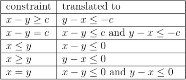
There are other constraints that can be easily translated and integrated

to this graph model. Table 3.1 gives a few of the common constraints that

can be translated to DL.

constraint translated to x−y≥c y−x≤ −c

x−y=c x−y≤c and y−x≤ −c x≤y x−y≤0

x≥y y−x≤0

x=y x−y≤0 and y−x≤0

Table 3.1: Table of constraints

Strict inequalities can also be handled with minor changes. We can always

(22)

on the type of numerical variables presented in the constraint. If they are all

integers,δ is precisely 1, e.g., we can change x−y <1 tox−y≤0 without any loss of precision. But if there are rationals or reals in the constraint,

δ has to be a very small value, small enough to not change the result of

evaluating the constraints.

It is a hard task to determine the value ofδin this case. However, we can

always say that the value ofδ is something very small like 1

∞. Representing this value in the computer is not possible, but we do not actually need it.

We can say thatδ is 1

∞, do the calculations using the symbolδ as a variable and see its real value when necessary.

Instead of evaluating a number c as itself, we think of it as a pair (c, k)

equivalent toc+kδ. The operations on the pair are like the ones we use for

equations (c+kδ), where cand k are known and δ is a variable. Only a few

operations will be necessary:

• (c1, k1) + (c2, k2)≡(c1+c2, k1+k2)

• (c1, k1)−(c2, k2)≡(c1−c2, k1−k2)

• c′

×(c, k)≡(c′ ×c, c′

×k)

Additionally, we can also compare two pairs because we know the value

of δ. We know that:

• (c1, k1)≤(c2, k2)≡(c1 < c2)∨(c1 =c2∧k1 ≤k2)

After mounting a graph with the entire set of diﬀerence logic constraints

we can observe many interesting facts. The following subsections will describe

(23)

3.2.1 Dependency

If two variables x and y don not depend on each other, there will not be a

path fromx toy neither a path fromy tox. In graph theory, a path fromx

toy is a set of edges that connect x toy.

A variable x may depend on another variable y either directly or

indi-rectly. In the ﬁrst case, there will be an edge from x to y and thus a path

fromxto y. In the second case, there will be a path from x toy that

repre-sents a combination of the constraints in the path and the length (or sum of

the edges cost) indicates the relationship between the variables.

For instance, take two constraints x−y ≤ −1 and y−z ≤ −2. The

combination of them (x−z≤ −3) show the indirect dependency between x and z. The graph representation for this example can be seen in Figure 3.2.

Figure 3.2: Direct (x−y ≤ −1 and y−z ≤ −2) and indirect (x−z ≤ −3) dependency of variables.

3.2.2 Strongest Constraint

The Strongest Constraint is related to a pair of variables. As the name suggests, it is the strongest constraint that can be created (or extracted)

(24)

y−x≤c1 is the strongest constraint related toyand x, that means that we

cannot extract any other constrainty−x≤c2 wherec2 < c1.

If there is a path from x to y, the shortest path len (the shortest path

in our case is related to the sum of the edges cost and not to the number

of the edges) from x to y gives the strongest constraint, related to x and y

(y−x ≤ len), that it is possible to create from the given facts. It means that y must be at mostx+len.

For instance, the following set of constraints are represented by the graph

in Figure 3.3: y−x≤ −1,z−x≤ −2,w−y≤ −3,w−z ≤0 andy−z ≤0.

The strongest constraint that we can build betweenx and wis w−x≤ −5, built from the shortest path from x tow (that goes throughz and y).

Figure 3.3: The strongest constraint related to two variables (vertices) can be build from the shortest path between them. In the ﬁgure, we have three strongest constraints (w −x ≤ −5, w− z ≤ −3 and y −x ≤ −2) that are derived from the shortest path and are not given in the set of original constraints.

3.2.3 Unsatisﬁability

A set of constraints is unsatisﬁable if there is a contradiction, e.g., x−y ≤ −1∧x−y≥2. If there is no combination of constraints that can make the

(25)

Theorem 1 There is a negative cycle in the graph if and only if the problem

is unsatisﬁable.

Proof. If there is a negative cycle in the graph it means that there are two vertices x and y in the cycle where the shortest path from x to y costs

−∞and the shortest path fromy tox is also−∞. That is possible because since the shortest path is related to the length (sum of the weights), and not

the number of edges, we can take the same edge many times. So, we have

x−y ≤ −∞ and y−x ≤ −∞, that implies: x−y≤ −∞ and x−y ≥ ∞, and thus a contradiction.

For the other half, if the problem containing only diﬀerence constraints is

unsatisﬁable it is because we have something such asx−y≤c1∧x−y≥c2,

wherec1 < c2. The ﬁrst literal implies that we have a path fromy toxwith

length c1 and the second one (can be changed to y−x ≤ −c2 implies that

we have a path from x to y with length −c2. So, we have a cycle (x, y, x)

with lengthc1 + (−c2). We know that c1 < c2 ⇒c1−c2<0. Therefore the

length of the cycle is negative.

After looking for negative cycles, we do not need to check for satisﬁability.

In case no negative cycle is detected the problem is satisﬁable.

Figure 3.4 shows a scenario where there is a negative cycle. The proof

for the unsatisﬁability (or conﬂict set) can be constructed from the edges

in the negative cycle, the combination of these constraints will lead to a

contradiction likex−y≤ −∞ and x−y≥ ∞.

3.2.4 Equality Between Variables

Theorem 2 Two variables x andy are equal if and only if the shortest path

(26)

Figure 3.4: Graph with a negative cycle. The set of constraints representing it is unsatisﬁable. The proof is the edges from the negative cycle: z−x≤0, y−z ≤0 and x−y≤ −1.

Proof. That is easy to see, with the knowledge that we presented so far, we know that the constraints representing these two shortest paths are

x−y ≤ 0 and y−x ≤ 0 (which is the same as x−y ≥ 0). Thus, from x−y ≤0 and x−y≥0 we have x−y= 0 (orx=y).

For the other half of the theorem, if we have two variables that are equal,

x and y, we have: x = y ⇒ x− y = 0 ⇒ x− y ≤ 0 ∧x −y ≥ 0 ⇒

x−y ≤ 0∧y−x ≤ 0. These last two represents the shortest paths with length 0. They cannot be stronger because otherwise the problem would be

unsatisﬁable.

Figure 3.5 shows an example where an equality is found using shortest

path information.

x−y≤0∧y−x≤0⇒x=yis exactly the way back from understanding

a constraint like x = y showed in Table 3.1. The diﬀerence is that this

(27)

Figure 3.5: Graph made from 3 constraints: z −x ≤ −1, y−z ≤ 1 and x−y ≤0. An equality can be found in this graph: x = y.

3.3 Conclusion

We presented diﬀerence logic and its graph model. We showed some

in-teresting properties that allow us to present, in Chapter 4, algorithms for

the decision procedure. We know, along other things, that we can check

for satisﬁability using algorithms for negative cycle detection. Additionally,

the theorem of equality between variables will give us enough knowledge to

(28)

Chapter 4 Decision Procedure for

Diﬀerence Logic

A decision procedure is a method to solve a decision problem, where the

expected answer isyes orno. In our case, a decision procedure will decide if a set of formulas is satisﬁable or not, i.e, if there exists an interpretation of

variables, functions and predicates that makes true every formula in the set.

For a decision procedure to work well in a Nelson and Oppen combination

framework and produce some worthy results, it should take some

require-ments in consideration. In this chapter, we will explain these requirerequire-ments

and show how the algorithms for implementing them work.

The work here was implemented in the theorem prover haRVey [8, 11].

Everything in the following sections is related to this implementation.

4.1 Requirements

A few things are necessary to the decision procedure beyond returning the

status of satisﬁability. They are requirements for the correct integration with

(29)

Chapter 4. Decision Procedure for Diﬀerence Logic 22

the Nelson and Oppen combination framework in a theorem prover.

There are a few basic requirements that are necessary. The decision

procedure needs to be correct, i.e., it should always return the correct status

of satisﬁability. It should terminate, i.e., it cannot run for an undeterminable

amount of time.

The other requirements will be presented in the following subsections.

The desirable requirements are conﬂict set generation, premisses,

incrementabil-ity. They can be considered accessory because the prover can still give the

correct status of satisﬁability without them, but they are useful for

improv-ing eﬃciency. The mandatory requirement is equality generation, that is

fundamental for the Nelson and Oppen combination framework.

4.1.1 Conﬂict Set Generation

Given a set of constraints, if the decision procedure detects that the problem

is unsatisﬁable then a proof is necessary. We call proof any subset of the

constraints that is unsatisﬁable. It can optionally contain the explanation of

how rules were applied to get the status. It is useful for the user to understand

if there is something wrong, so he/she can reformulate the problem when

necessary. It also can be used to conclude that the result is as expected.

The proof may also be useful when used by the theorem prover to reduce

the time of execution. If it is detected that an already proved unsatisﬁable

subset of constraints is in the current problem the prover can stop running

the problem, because it is known that it is unsatisﬁable. This can be realized

by the SAT solver by adding a so called conﬂict clause, corresponding to the

negation of the literals found in the proof.

As a simple example, given the set of constraints:

(30)

The decision procedure should be able to detect that the problem is

un-satisﬁable due to:

x−y≤0;y−x≤ −1

4.1.2 Equality Generation

One of the main assumptions of the Nelson and Oppen combination

frame-work is the equality propagation between decision procedures. Every

deci-sion procedure in the framework should be able to detect equalities, so these

equalities may be propagated to the other decision procedures. That will

allow the theorem prover to infer about combined theories.

Without the equality propagation, the isolated decision procedures may

not have enough information to ﬁnd satisﬁability of some combined theory.

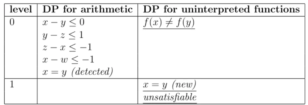
For example, given the formula:

x−y≤0∧y−z ≤1∧z−x≤ −1∧x−w≤ −1∧f(x)=f(y)

The Nelson and Oppen scheme could split the formula and send

con-straints to two decision procedures, one to deal with the arithmetic theory

and another one to deal with uninterpreted functions. A possible scenario is

shown in Table 4.1.

The Table 4.1 shows that, in a ﬁrst moment, working alone, the

deci-sion procedures cannot detect the unsatisﬁability. However, an equality is

detected and propagated to the other decision procedure. This new

informa-tion allows the decision procedure for uninterpreted funcinforma-tion to detect the

(31)

level DP for arithmetic DP for uninterpreted functions

0 x−y≤0 f(x)=f(y) y−z ≤1

z−x≤ −1 x−w≤ −1 x=y (detected)

1 x=y (new)

unsatisﬁable

Table 4.1: Example of equality generation.

Integer Case

For non-convex theories, such as integer diﬀerence logic, it is also necessary to

generate disjunction of equalities (see Nelson and Oppen [14]). To illustrate

the necessity, consider the following set of constraints as example, where the

variables can only have integer values.

¬(x−y= 1) ¬(x−y= 2)

x−y≥1

x−y≤2

The ﬁrst two constraints are not handled by the decision procedure for DL

because they are not part of the theory. They will be handled by another DP.

The decision procedure for DL should be able to generatex−y= 1∨x−y= 2. If such disjunction is not generated, the contradiction (¬(x−y= 1)∧ ¬(x−

(32)

4.1.3 Premisses

When unsatisﬁability is detected, the proof may contain constraints that are

not in the original problem. That is because a decision procedure may have

constraints generated internally by the theorem prover, like, for example, the

detected and propagated equalities.

For constructing a consistent proof, the original constraints are necessary.

It is possible to track them by knowing the premisses of a constraint. The

premisses of a constraint are the constraints used to generate it.

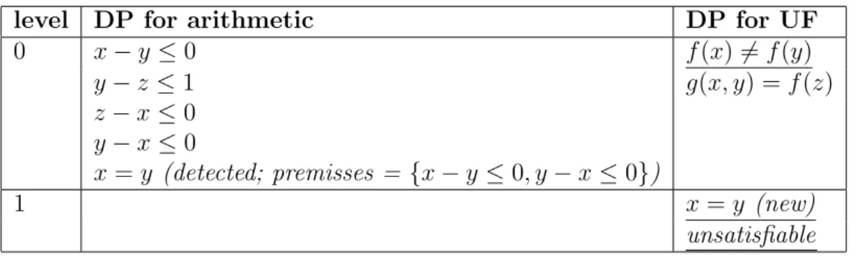
For example, from the following formula, we extract the information

pre-sented in Table 4.2:

x−y≤0∧y−z ≤1∧z−x≤0∧y−z≤0∧f(x)=f(y)∧G(x, y) =f(z)

level DP for arithmetic DP for UF

0 x−y≤0 f(x)=f(y)

y−z ≤1 g(x, y) = f(z)

z−x≤0 y−x≤0

x=y (detected; premisses = {x−y ≤0, y−x≤0})

1 x=y (new)

unsatisﬁable

Table 4.2: Example of premisses.

In the decision procedure for uninterpreted functions (U.F.), the problem

is detected to be unsatisﬁable due to f(x) = f(y) and x = y. But the information x = y is not present in the original formula, so giving it in the

proof might not be interesting.

The decision procedure that generates the new constraint should also be

(33)

when the unsatisﬁability is detected using premisses information, we can

construct as proof:

x−y≤0∧y−x≤0∧f(x)=f(y)

4.1.4 Incrementability

When testing a set of constraints, a decision procedure may detect that a

subset of the constraints is unsatisﬁable. In that case, it is not necessary

to continue executing the decision procedure since the entire problem is also

unsatisﬁable.

Therefore, a decision procedure that works incrementally (checking the

satisﬁability each time a new constraint is received) may be more eﬃcient.

But, for that, a good incremental algorithm is necessary. It should remember

the previous status and when a new constraint comes, it should use previous

calculated information to reduce the computation of the new check.

Moreover, even after testing the entire set of constraints originally

as-signed by the Nelson and Oppen scheme, new constraints may come. These

new constraints, such as the variable equalities, produced by other decision

procedures, have to be incorporated and a new check for satisﬁability is

nec-essary. The set of constraints to test is the same, except for the new one.

For a large problem, this might happen a considerable number of times. So,

using an incremental algorithm for checking the consistency of the new set

is also very desirable for this situation.

Another importance of using incrementability comes when testing

formu-las leads to several checking paths. When disjunction is present in a formula,

a SAT-solver, using techniques such as DPLL [9, 10], may have to test

re-peatedly some sets of constraints to verify the satisﬁability of the original

(34)

techniques will keep track of paths and occasionally, when testing another

path is necessary, backtrack to a common point in the path and do not redo

subproblems over and over again.

As a consequence of having to come back in the path, i.e., remove some

constraints from the set and later add others, the incremental algorithm also

should be backtrackable. It should be able to remove the last constraint

added and then reestablish the previous state eﬃciently, when the removed

constraint was not in the set.

As an example of this situation and the necessity of having an incremental

and backtrackable algorithm, consider the following formula:

(x−y ≤0∨x−y≤ −1)∧(y−z ≤0∨y−z≤ −1)∧(z−x≤ −1∨z−x≤ −2)

For testing the formula in CNF (Conjunctive Normal Form - a formula

is in CNF if it is a conjunction of clauses, where a clause is a disjunction of

literals), a SAT-solver will set values (true or false) to the literals to make

each clause true. In this example, where all the literals are diﬀerent from each

other, in the worst case scenario it may be necessary to explore 2×2×2(= 8) paths to check diﬀerent sets of constraints. In Figure 4.1, there is a simulation

of a scenario where a SAT-solver based on DPLL using a decision procedure

for arithmetic checks the formula.

In an incremental and backtrackable algorithm, for every new constraint

added, a satisﬁability check is done. If there is a contradiction in the current

set, it is not necessary to continue and a backtrack to a common point is

done. From this point, the process continues and the SAT-solver resumes

assigning appropriated values to the literal to ﬁnd out if the original formula

(35)

Figure 4.1: Paths to check (from the previous formula). In this case, it was necessary to take 4 paths to conclude that the formula is unsatisﬁable. After events 9 and 12 contradictions are early found so there is no necessity to continue checking the branch.

4.2 Algorithms for the Diﬀerence Logic

De-cision Procedure

With these requirements in mind, the following subsections will explain how

algorithms for a diﬀerence logic decision procedure work. Many diﬀerent

algorithms can be used for the same purpose. We decided to describe those

(36)

4.2.1 Satisﬁability Checking

As shown in the Section 3.2.3, a set of constraints is unsatisﬁable if, and

only if, the graph made from the constraints has a negative cycle. The

classical algorithm to check if a graph has a negative cycle is the

Bellman-Ford algorithm [3, 12]. Algorithm 2 shows its pseudocode. Although it

does not match our requirements for incrementability, it is a good reference

algorithm.

input :G= (V, E) :Graph, source:V ertex

output:hasN egativeCycle:Boolean

// Initialize graph

foreach vertex v in V do

1

v.distance=IN F IN IT Y;

2

v.predecessor =N U LL;

3

end

4

V[source].distance= 0;

5

// Relax edges repeatedly

for i= 1 to |V|do

6

foreach edge e in E do

7

u=e.source;

8

v =e.destination;

9

if v.distance > u.distance+e.weightthen

10

v.distance=u.distance+e.weight;

11

v.predecessor =u;

12

// Check for negative-weight cycles

if i== |V| then

13

return hasN egativeCycle=true;

14 end 15 end 16 end 17 end 18

return hasN egativeCycle=f alse;

19

Algorithm 2: BellmanFord

(37)

graph and also looks for negative cycles. It is a non incremental algorithm

and runs inO(V E), where V is the number of vertices and E is the number

of edges.

The idea of Bellman-Ford algorithm is based on relaxing the estimated

distance between the source and all the other vertices. After the cycle i

from the For loop, v.distance will contain the shortest path from source to v using at most i edges. After the |V| −1 cycle, the distances from source to the vertices should be the shortest path. The exception is when there is

a negative cycle reachable fromsource. In such cases, the shortest path can

always be reduced by going through the cycle an inﬁnite number of times.

4.2.2 Incremental Satisﬁability Checking

To be worth using, an incremental algorithm should be more eﬃcient than

a static (non incremental) one. In this subsection we present an incremental

satisﬁability check algorithm developed by us, Algorithm 3. It can be

imple-mented using a heap with complexityO(V+E′ logV′

), whereV is the number

of vertices,V′

is the number of vertices that have their distance changed in

the algorithm and E′

is the number of outgoing edges of theV′

vertices.

The idea of the algorithm is to search in the graph for the vertices that

may have their distances changed due to the last added edge. The distance

is the length of the shortest path from an arbitrary source vertex. For this

purpose and for simplicity, anartiﬁcial vertexcan be created to be the source vertex. It will connect all the other vertices with an unidirectional edge with

weight 0. The original system will be unsatisﬁable if, and only if, the slightly

modiﬁed one (with the artiﬁcial vertex) is.

The algorithm starts by checking if the new edge will improve the distance

(38)

input :G= (V, E) :Graph, e :Edge

output:hasN egativeCycle:Boolean

// Initialize Δ

foreach vertex v in V do

1

Δ(v) = 0;

2

end

3

// Initial check

u=e.source, v =e.destination;

4

Δ[v] = (u.distance+e.weight)−v.distance;

5

if Δ[v]<0 then

6

Q= NewHeap();

7

Q.InsertOrImprove(v,Δ(v), u);

8

// Improving Search

while Q.Empty()==f alsedo

9

v, delta, u=Q.RemoveMin();

10

v.distance=v.distance+ Δ[v];

11

v.predecessor =u;

12

foreach outgoing edge i of v do

13

t=i.destination;

14

if (v.distance+i.weight)−t.distance <Δ[t]then

15

if t ==e.source then

16

return hasN egativeCycle=true;

17

else

18

Q.InsertOrImprove(t,Δ[t], v);

19 end 20 end 21 end 22 end 23 end 24

return hasN egativeCycle=f alse;

25

Algorithm 3: IncrementalNegativeCycleDetection

greedily picking the vertex in the heap that will have its distance improved

the most. The improvement is the diﬀerence between the new and old value

of distance. It is assumed that, when a vertexvis improved, its neighbors will

(39)

vertex has its distance improved, it is done by the path that will mostly

improve the distance. Therefore, each vertex should have their distance

improved at most once. The exception is when there is a negative cycle.

A negative cycle happens if and only if the e.source distance improves.

Because if e.source improves that means that e.destination will improve

again, so a cycle is present.

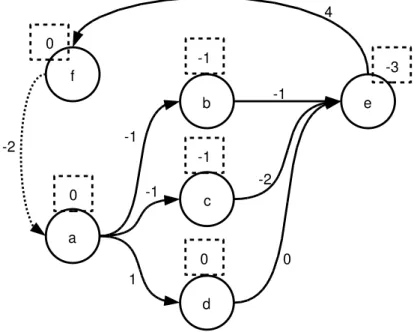
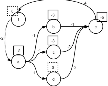
Figure 4.2 shows an example of an arbitrary set of constraints. The graph

representation is shown with the distance information of each variable in the

squares. A new constraint is added, a−f ≤ −2. From that, we show the

behavior of the Algorithm 3 in the Table 4.3.

Figure 4.2: Graph representation of an arbitrary example, state before con-straint insertion.

At each step, the chosen vertex from the heap will have its distance

improved (only once) by the shortest path. When the source vertex f is

(40)

shows the ﬁnal state of this example.

Time Current vertex Heap (vertex, improvement)

0 f (a,−2)

1 a (b,−2)

(c,−2) (d,−1)

2 b (c,−2)

(d,−1) (e,−1)

3 c (e,−2)

(d,−1)

4 e (d,−1)

(f,−1) // negative cycle

Table 4.3: Behavior of the Algorithm 3 running on Figure 4.2.

(41)

4.2.3 Conﬂict Set Construction

When unsatisﬁability is detected, a proof is necessary. The proof is the set

of constraints that generated a conflict (the conflict set). A minimal conflict

set can be obtained by the constraints that form the negative cycle.

The algorithm for checking the unsatisﬁability keeps the predecessor of

the vertices while updating the shortest path distances and doing the search

for a negative cycle. So, if a negative cycle is detected, it is only necessary

to go through the cycle, by using the predecessor, and collect the constraints

associated to the edges. A pseudo-code for this is showed in Algorithm 4.

input :G= (V, E) :Graph, e :Edge

output:s :Set of constraints

v =e.source;

1

s.Insert(e.constraints);

2

while v =e.destination do

3

s.Insert(Edge(v.predecessor, v).constraints);

4

v =v.predecessor;

5

end

6

return s;

7

Algorithm 4: ConﬂictSet

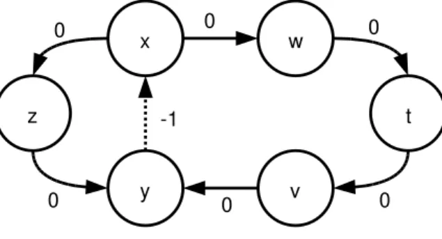
When a new edge is added, more than one negative cycle may arise. See

for instance, Figure 4.4. In this case, it is possible to return more than one

minimal conﬂict set. But the algorithm will return the ﬁrst negative cycle

found.

4.2.4 Equality Generation

It was shown in Section 3.2.4 that, in our graph model, two variablesx and

y are equal if, and only if, the lengths of the shortest path betweenx and y

(42)

Figure 4.4: In this graph, representing a set of constraints, two negative cycles are found after the edge (y, x,−1) is added. The cycles are {y, x, z, y} and {y, x, w, t, v, y}. Any of them can be used to construct the conﬂict set.

Algorithm 5 (inspired by [13]) shows how to generate equalities without

explicitly calculating the shortest path between each pair of vertices in the

graph. It assumes that no negative cycle is present.

It is not an incremental algorithm, because it redoes every calculation

each time it is called, i.e., each time a new constraint is added. It can be

implemented with complexity O(V ∗logV +E), where E is the number of edges in G and V is the number of vertices inG.

The algorithm starts by mounting a graphG′

from the edges whereslack is equal to zero. An edgeehasslack(e)zero wheneis part of a shortest path between the artiﬁcial variable and the destination of e (e.destination). We deﬁneslack(e) by:

slack(e) =e.source.distance−e.destination.distance+e.weight

Any cycle C = [v1, v2, ..., vn] in G′ will have its length equal to zero. To

see that, let us ﬁrst make some deﬁnitions:

• v1..vn are vertices

(43)

input :G= (V, E) :Graph

output:s :Set of equalities

// Mount graph G′

from E′

and its vertices

foreach edge e from E do

1

if e.source.distance - e.source.distance + e.weight == 0 then

2

E′

.Insert (e);

3 end 4 end 5 G′

= Graph (E′ );

6

// Look for equalities in each SCC

SCCs=G′

.FindStronglyConnectedCompenents();

7

foreach scc in SCCs do

8

sort vertices of scc by distance;

9

for i= 1 to |scc| −1do

10

if vi.distance==vi+1.distance then

11

eq =Equality(vi, vi+1);

12

if NotGeneratedYet(eq) then

13

s.Insert (eq);

14

eq.SetPremisses(FindPremisses(G′

, vi, vi+1));

15 end 16 end 17 end 18 end 19 return s; 20

Algorithm 5: GenerateEqualities

• w(vi, vi+1) is the weight of the edge betweenvi andvi+1. It is a shortcut

for Edge(vi, vi+1).weight

• d(vi) is the length of the shortest path between a vertex (theartiﬁcial

one) and vi. It is a shortcut for vi.distance

The length of a cycleC is the sum of the edge weights in the cycle. More

formally we have:

(44)

Adding the terms +d(vi) and −d(vi) will not change the result of the

length, because they cancel each other. So, doing this we have:

Length(C) =d(v1)−d(v1) +d(v2)−d(v2) +...+d(vn−1)−d(vn−1) +

w(v1, v2) +w(v2, v3) +...+w(vn−1, v1);

Now, we just rearrange the terms to see more precisely the next step. It

will be like this:

Length(C) = [d(v1)−d(v2) +w(v1, v2)] + [d(v2)−d(v3) +w(v2, v3)] +...+

[d(vn−1)−d(v1) +w(vn−1, v1)];

We can see that [d(vi)−d(vi+1) +w(vi, vi+1)] is exactly the slackdeﬁned

before. We know that in G′

, all the slacks are 0 because of the way G′ was

mounted. So evaluating the expression we have:

Length(C) = 0

The next step in the algorithm is to get the Strongly Connected

Compo-nents (SCCs). We call a graph a strongly connected component (SCC) if for

every pair of verticesu and v there is a path from uto v and also fromv to

u. The SCCs of a graph are the maximal strongly connected subgraphs of

the graph.

Any two vertices in a SCC of G′

will be in a cycle of length zero and the

path between them is also the shortest path in the original graph G. That

is the primary condition for two variables to be equal. They need to be in a

cycle of length zero. Based on that, every pair of vertices in each SCC are

potential candidates to be equal.

For checking if two variables v1 and vn are equal without having to

(45)

distance information that we keep when looking for negative cycles. The

shortest paths between them have to be zero, so mathematically we have:

0 = w(v1, v2) +w(v2, v3) +...+w(vn−1, vn);

0 =w(vn, vn−1) +w(vn−1, vn−2) +...+w(v2, v1);

We know by the deﬁnition ofslackthat: slack(vi, vi+1) = d(vi)−d(vi+1)+

w(vi, vi+1). Knowing that the slacks in G

′

are zero, we have: w(vi, vi+1) =

−d(vi) +d(vi+1). Thus, developing the previous expressions:

0 = −d(v1) +d(v2)−d(v2) +...+d(vn−1)−d(vn−1) +d(vn);

0 = −d(vn) +d(vn−1)−d(vn−1) +...+d(v2)−d(v2) +d(v1);

Simplifying everything:

0 = −d(v1) +d(vn);

0 = −d(vn) +d(v1);

Therefore, in any SCC of G’, two variables v1 and vn are equal if they

have the same distance value, i.e., d(v1) = d(vn).

Summarizing, Algorithm 5 will look in each SCC of G′

for every pair of

vertices. If they have the same distance, an equality is found. If this equality

is not new, it is added to the set of new equalities generated to be returned.

Additionally, the set of premisses is associated to it.

Algorithm 6 shows a pseudo-code for ﬁnding the strongly connected

com-ponents (SCCs) of a graph. Its complexity is linear in the number of edges

[20].

It runs a series of depth ﬁrst searches (DFS) using a graph G starting

from each not visited vertex. Later, another series of DFS is done, but now

using the transpose set of edges ET

(46)

input :G= (V, E) :Graph

output:s :Set of SCC

// Mount GT

by creating new edges changing the source and destination of E

foreach edge e in E do

1

ET

.Insert(Edge(e.destination, e.source));

2

end

3

GT

= Graph(V, ET

);

4

// First DFS

foreach vertex v of V do

5

if v.visited == false then

6

v.visited=true;

7

DFS(G, v);

8

end

9

end

10

// Second DFS, by decreasing finish time of the first DFS

Sort V by the decreasing time of v.timeF inished;

11

foreach vertex v of V do

12

if v.visited == false then

13

v.visited=true;

14

DFS(GT

, v);

15

s.Insert(each vertex visited now);

16

end

17

end

18

return s;

19

Algorithm 6: FindStronglyConnectedComponents

order of “ﬁnished visit” time of the ﬁrst DFS. In this second series of DFS,

all the vertices reachable on each DFS belong to the same SCC.

Algorithm 7 shows how a depth-ﬁrst search (DFS) works. The DFS

is a search algorithm that explores each branch as deep as possible before

backtracking, see, e.g., [6]. Starting in a vertexv, it will mark as visited every

vertex reachable from v. Additionally, when a vertex u cannot continue the

(47)

visit” time set.

input :G= (V, E) :Graph, v :V ertex

foreach outgoing edge e of v do

1

if e.destination.visited == false then

2

e.destination.visited =true;

3

DFS(G, e.destination);

4

end

5

end

6

v.timeF inished =NextTime();

7

Algorithm 7: DFS

4.2.5 Premisses Information

Given an equality between two variables, the premisses of this equality are

the constraints that generated the equality. We know that two variables u

andv are equal if the length of the shortest paths fromu tov and fromv to

uare 0.

Then, for constructing the set of premisses, it is only necessary to extract

the constraints related to each edge in the shortest path between u and v

and betweenv and u. Algorithm 8 shows a pseudo-code for this.

input :G= (V, E) :Graph, u:V ertex, v :V ertex

output:s :Set of Constraints

// Update the predecessor BFS(G, u, v);

1

BFS(G, v, u);

2

// Get the set of premisses

s =GetConstraints(G, u, v) +GetConstraints(G, v, u);

3

return s;

4

Algorithm 8: FindPremisses

(48)

starting from v. That will save inG the predecessors corresponding to (one

of) the shortest paths between u and v and between v and u. Later, this

information is used to go through the paths and collects the constraints

associated to each edge in the paths.

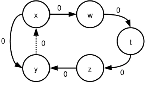
An equality can have more than one set of minimal premisses (see Figure

4.5 for an example). Using BFS to ﬁnd the shortest path (number of edges)

will allow to ﬁnd the minimumset of premisses.

Figure 4.5: In this graph, representing a set of constraints, an equality can be found after the edge (y, x,0) is added. Two sets of premisses can be returned as a proof for x = y (there are two shortest paths with length 0): {x−y ≤0, y−x≤0}and{x−y≤0, w−x≤0, t−w≤0, z−t ≤0, y−z ≤0}.

The BFS is a search algorithm that can be used to ﬁnd the shortest

path (related to the shortest number of edges), see, e.g., [6]. It executes the

search by visiting all neighbors ﬁrst and then visiting the neighbors of the

neighbors and so on, until it ﬁnds the goal. For this, it uses a queue (FIFO

- First In First Out). Algorithm 9 shows a pseudo-code. The goal is to ﬁnd

the destination vertex.

Algorithm 10 shows a pseudo-code for getting the constraints in a path.

It is similar to the Algorithm 4 that gets the conﬂict set. It just follows

the path using the predecessor information that was previously recorded and

(49)

input :G= (V, E) :Graph, source:V ertex, destination:V ertex

source.predecessor =N U LL;

1

Q.Add (source);

2

while Q.Empty() == false do

3

u=Q.Remove();

4

foreach outgoing edge e of u do

5

if e.destination.visited == false then

6

e.destination.visited =true;

7

e.destination.predecessor=u;

8

if e.destination == destination then

9

return;

10

end

11

Q.Add(e.destination);

12 end 13 end 14 end 15

Algorithm 9: BFS

input :G= (V, E) :Graph, source:V ertex, destination:V ertex

output:s :Set of constraints

while source=destinationdo

1

pred =destination.predecessor;

2

s.Insert(Edge(pred, destination).constraints);

3

destination=pred;

4

end

5

return s;

6

Algorithm 10: GetConstraints

4.3 Conclusion

This chapter described the requirements to build a decision procedure for

dif-ference logic and presented some algorithms for it. There are some desirable

and necessary requirements that comes specially from Nelson and Oppen

framework necessities and observations. For the algorithms, some known

(50)

al-Chapter 4. Decision Procedure for Diﬀerence Logic 43

gorithm for satisﬁability check was described. Generating the disjunction of

(51)

Chapter 5 Implementation details

The Chapter 4 explained what is necessary to write a decision procedure

(DP) for diﬀerence logic (DL). An implementation integrated to the theorem

prover haRVey [8, 11] was done following that speciﬁcation. However, there

are a few extra details that only comes when implementing the decision

procedure.

This chapter will explain exactly what kinds of constraints the

imple-mentation handle and how they are handled. It also describes the minor

diﬀerences presented in this implementation, as well as its behavior inside

haRVey and some use cases.

5.1 Benchmark

Arithmetic is a vast theory. Even for the segment of diﬀerence logic, we

have to deﬁne precisely what kinds of constraint we should handle taking in

consideration the capacity of the decision procedure.

The primary goal is to handle the benchmarks from SMT-LIB [17], the

Satisﬁability Modulo Theories Library. Its major goal is to establish a

(52)

Chapter 5. Implementation details 45

brary of benchmarks for satisﬁability of formulas with respect to background

theories for which specialized decision procedures exist. The constraints that

appear in these benchmarks can be summarized in the Table 5.1.

The constraints are rewritten for simplicity and eﬃciency. We work with

only one predicate (≤) instead of four (≤,≥, <, >). That allows the SAT

solver to infer about things like a ≤ b∧a > b, that would be rewritten to

a≤b∧¬(a≤b), and detect the contradiction without the necessity of calling the DP.

constraint rewrite to x−y≤c x≤y+c x−y≥c y+c≤x x−y < c ¬(y+c≤x) x−y > c ¬(x≤y+c) x−y=c x=y+c x−y=c ¬(x=y+c) x≤y x≤y

x≥y y≤x x < y ¬(y≤x) x > y ¬(x≤y) x=y x=y x=y ¬(x=y)

Table 5.1: Table of constraints and their rewrite

haRVey, using the DP for DL, should be able to give the correct answer

to any set containing those constraints. The negation of equality constraints

will not be directly received by the DP. That is because haRVey follows the

combination framework of Nelson and Oppen, and it will ﬁlter the constraints

and give only some of them to the DP. But another DP will handle it and

(53)

5.2 Handling Constraints

Additionally to the benchmark, the DP will have to handle data created

internally by haRVey. We call them clues. They are constraints or terms of

a constraint. There are four kinds of clues that the DP for DL may receive:

abstract Any term of a constraint that has a meaning for diﬀerence logic, i.e.,

numbers and sums. Examples: 0;x+ 2.

predicate Any constraint that has the predicate ≤. Examples: x≤y+ 1;¬(z ≤

x).

merge A equality between clues that will merge two class representants.

Ex-amples: x=y;z =y+ 2.

replace The same as merge, but one of the clues are not known by the DP.

Every clue has a class representant that is also a clue. All the clues with

the same class representant are equal. A clue c has its class representant

changed when an equality is found between cand another clue by some DP.

Figure 5.1 shows a scheme for handling the clues received by the DP for

DL. The idea is to keep a table that associate a number to a clue whenever

there is a direct or indirect relationship between them. The second step is to

update the graph and to use the algorithms presented in Chapter 4. Also,

when we can infer about something, we save the premisses to be able to

construct the proof later. This is omitted in the diagram for simplicity.

Only the top most symbols of the clues are checked. Everything else

is treated as a variable. Therefore, if constraints from other theories are

received, like for example, car(cons(w, l)) ≤ f(z) + 1, they will be treated as if they were X ≤ Y + 1, i.e, car(cons(w, l)) and f(z) are treated as they

(54)

Figure 5.1: Decision diagram showing how to handle the clues.

5.3 Building the Graph

All the information received in the clues will be transmitted to the graph

that will run the main algorithms. The numbers will be in the graph as the

(55)

Let us take as example the set of constraints: x ≤ y + 1;x = y;y ≤

x+ (−1). From them, the DP for DL will receive a set of clues. They are

shown in Table 5.2

time clue type

1 1 abstract

2 y+ 1 abstract

3 x≤y+ 1 predicate

4 x=y merge

5 −1 abstract

6 x+ (−1) abstract 7 y≤x+ (−1) predicate

Table 5.2: Example of clues received by the DP for DL.

At each step, we follow the diagram in Figure 5.1. If the graph is changed,

a satisﬁability check is done. If the problem is detected unsatisﬁable, we can

stop the process.

At the ﬁrst moment, when the clue “1” is received, the information will

not go immediately to the graph. When the sum “y+ 1” appears, the graph

will start being built. If we follow the diagram in Figure 5.1, we will “update

the graph with a = a1 +a2”. a is the representant of y+ 1, that is y+ 1

itself, a1 is the representant of y, y itself, and a2 is the number 1. So the

graph will be updated with something like, (y+ 1)−(y) = 1, or, as we saw

before, (y+ 1)−(y) ≤1∧(y)−(y+ 1) ≤ −1. We can see the graph after receivingy+ 1 in Figure 5.2.

Adding to the graph the information (y+ 1) = (y) + (1), may look

redun-dant, but it provides an easier way to generate the important equalities. If we have only two constraints likea=b+ 1 andb=c+ 1, it is not important

to the other decision procedures to know that a = c+ 2, that is because

(56)

Figure 5.2: Graph after receiving the second clue y+ 1.

unnecessary as it will not help. It is only important to generate equality

between information that are already known by the others DPs.

Doing as described will add to the graph all the known (by the others

DPs) information. So we can ﬁnd the interesting equalities by just following

Algorithm 5.

After receiving the third clue x ≤ y+ 1, following the diagram, we will

“update graph witha1−a2≤0”. a1 is the representant ofx, that isxitself, and a2 is the representant of y+ 1, that isy+ 1 itself. So the graph will be

updated with (x)−(y+ 1)≤0. We can see the result in Figure 5.3.

Figure 5.3: Graph after receiving the third clue x≤y+ 1.

The result is slighted diﬀerent from the one if we had updated withx−y ≤

(57)

path between y and x. Also, by doing as described, we avoid looking deep

in the term, simplifying the process.

The fourth clue x = y is a merge. The representant of x will now be

the same as the representant of y. So we add the information in the graph:

x−y ≤0∧y−x≤0. We can see the result in Figure 5.4.

Figure 5.4: Graph after receiving the fourth clue x=y.

Let us assume that the representant ofxchanged toy, in the fourth step.

The step 5 will just update the table that makes the relationship between

clues and numbers.

The step 6 will be similar to the second one, the diﬀerence is that now

the representant ofxwill point to another variable (y). We can see the result

in Figure 5.5.

Finishing the example, in the step 7, we update the graph and detect a

negative cycle. The ﬁnal graph is shown in Figure 5.6.

5.4 Conclusion

In this chapter, we explained the details that make the implementation a

bit diﬀerent from theory. We described the benchmark and presented a new

Deciding di&#64256;erence logic in a Nelson-Oppen combination framework

Deciding diﬀerence logic in a Nelson-Oppen

combination framework

Deciding diﬀerence logic in a Nelson-Oppen

combination framework

Contents

Chapter 1

Introduction

Chapter 2

Techniques for SMT solving

2.1

Introduction

2.2

Nelson and Oppen Combination

Frame-work

2.3

Sat-Solver with DPLL

2.4

Conclusion

Chapter 3

Diﬀerence Logic

3.1

Introduction

3.2

Properties and Graph Representation

3.2.1

Dependency

3.2.2

Strongest Constraint

3.2.3

Unsatisﬁability

3.2.4

Equality Between Variables

3.3

Conclusion

Chapter 4

Decision Procedure for

Diﬀerence Logic

4.1

Requirements

4.1.1

Conﬂict Set Generation

4.1.2

Equality Generation

4.1.3

Premisses

4.1.4

Incrementability

4.2

Algorithms for the Diﬀerence Logic

De-cision Procedure

4.2.1

Satisﬁability Checking

4.2.2

Incremental Satisﬁability Checking

4.2.3

Conﬂict Set Construction

4.2.4

Equality Generation

4.2.5

Premisses Information

4.3

Conclusion

Chapter 5

Implementation details

5.1

Benchmark

5.2

Handling Constraints

5.3

Building the Graph

5.4

Conclusion

Deciding diﬀerence logic in a Nelson-Oppen combination framework