FUNDAC
¸ ˜
AO GETULIO VARGAS
ESCOLA DE P ´
OS-GRADUAC
¸ ˜
AO EM
ECONOMIA
Kym Marcel Martins Ardison
Nonparametric Tail Risk, macroeconomics and stock
returns: predictability and risk premia.
Kym Marcel Martins Ardison
Nonparametric Tail Risk, macroeconomics and stock
returns: predictability and risk premia.
Disserta¸c˜ao submetida a Escola de P´os-Gradua¸c˜ao em Economia como requisito par-cial para a obten¸c˜ao do grau de Mestre em Economia.
´
Area de Concentra¸c˜ao: Finan¸cas
Orientador: Caio Almeida
Ficha catalográfica elaborada pela Biblioteca Mario Henrique Simonsen/FGV
Ardison, Kym Marcel Martins
Nonparametric tail risk, macroeconomics and stock returns: predictability and risk premia / Kym Marcel Martins Ardison. - 2015.
58 f.
Dissertação (mestrado) - Fundação Getulio Vargas, Escola de Pós-Graduação em Economia.
Orientador: Caio Almeida. Inclui bibliografia.
1. Risco (Economia) 2. Análise de regressão. 3. Ações (Finanças). 4. Mercado financeiro. I. Almeida, Caio Ibsen Rodrigues de. II. Fundação Getulio Vargas. Escola de Pós-Graduação em Economia. III.Título.
Acknowledgements
First and foremost, I am grateful to Caio Almeida for the guidance and intellectual support throughout my master’s.
This dissertation benefited from discussions with Luiz Braido, whom taught me how to better express my ideas, seminar participants at Advanced Topics in Finance (FGV-EPGE) and at LACEA-LAMES conference.
Finally, I would like to thank my parents for the support during all my life and Leticia whom was by my side during all my time in EPGE.
Statement of Conjoint Work
Abstract
This paper proposes a novel way to estimate tail risk incorporating risk-neutral in-formation without making use of options data. Adopting a nonparametric approach we derive a risk neutral measure that correctly prices a chosen panel of stocks re-turns. We make use of this measure to define a tail risk factor as the price of a synthetic out-of-the money put option. Using 25 Fama-French size and book to market portfolios to estimate tail risk, we find that our factor has significant pre-dictive power when forecasting aggregate U.S. macroeconomic activity indexes and yield spreads. Impulse response functions also reveal that shocks in Tail Risk im-pact negatively employment and industrial production in the short-run. In addition, portfolios sorted by Tail Risk exposure reveal that when adopting a high minus low strategy, our factor presents a negative statistically significant excess return.
Contents
1 Introduction 8
2 Related Literature 10
3 Methodology 13
3.1 Asset Pricing Models: Minimum Distance Problem . . . 19
4 Empirical Results 20 4.1 The Data . . . 20
4.2 Empirical Features . . . 21
4.3 Stock Markets Returns . . . 24
4.4 Economic Predictability . . . 27
4.4.1 Business Cycles . . . 30
5 Conclusion 31
List of Figures
1 This figure presents the physical and implied risk neutral probabilities. In this example e set as our basis assets the 25 Fama and French equally weighted size and book to market portfolios and considered a 200 days
time span. γ =−3. . . 17
2 This figure presents the physical and implied risk neutral probabilities for a selected date setting γ =−3, the 25 Fama and French equally weighted size and book to market portfolios as our basis assets and 30 days in the estimation procedure. . . 18
3 This figure presents the Tail Risk (TR) time evolution from July 1926 to April 2014. Blue line indicate the actual tail risk series while red line indicate Hoddrick-Prescott filtered trend. Tail Risk was calculated using 25 Fama and French equally weighted size and book to market portfolios as basis assets considering a time span of one month (30 days) and γ =−3. 23 4 This figure presents the impulse response function on Employment and Industrial Production (for the manufacturer sector) based on a VAR es-timation (Bloom (2009)). The impulse response functions are relative to one standard deviation shock on tail risk. . . 28
List of Tables
1 The Data . . . 212 Tail Risk Correlations . . . 22
3 Tail Risk Beta-Sorted Portfolios: Endogenous Put . . . 26
4 Spread prediction . . . 29
5 Macroeconomic Indicator Regressions. . . 31
6 Correlations Between Tail Risk Measures . . . 36
7 Robustness ADS . . . 37
1
Introduction
It is now known that asset prices reflect a premium for disasters and other type of tail risks. Specially after the financial crisis in 2008, a considerable number of researchers turned their efforts to understanding how these risks influence the variance and equity risk premia. From an asset pricing perspective, a large branch of the literature seeks to estimate the jump risk premium implicit in option prices based on parametric jump-diffusion models for the evolution of stock prices1. From a macroeconomic point of view,
recent papers subsequent to Barro (2009) put an additional effort on the reconciliation of observed risk premium and consumption based models. Most importantly, both venues suggest that measuring tail risks is a particularly challenging task since large “jumps” in consumption or prices are, by nature, rare.
Coupled with this research effort to better understand tail events, regulators have recently shown special concern about the ability of traditional risk models to anticipate financial crises arguing that an effective way to access tail risk is mandatory now.2
Indeed, regulators’ concern strongly increased in recent years due to the effects of the subprime crisis. For instance, Andy Haldane, Executive Director of Financial Stability of the Bank of England, recently stated that “the fatter the tails of the risk distribution, the more misleading VaR-based risk measures will be” 3
.
In this paper, we contribute to the tail risk literature by focusing on risk neutral in-formation to provide a new measure of nonparametric tail risk. A frequent characteristic shared by most of the previous papers in this subject that choose to use risk neutral information is that their measures of tail risk are option data dependent. Being option dependent is in general good since options contain strong information on the expected values of the tails of the underlying assets, in particular short out of the money put options. However, unfortunately many markets around the world do not have well es-tablished option trading activity (in contrast to the U.S. market) and in such situations obtaining a time-varying tail risk measure can be extremely challenging. Our goal is to fill the gap that exists for such markets since our methodology relies only on the existence
1See Bates (2000), Pan (2002), Eraker (2004), and Broadie et al. (2009), among others.
2Regulators generally gauge market risk by Value-at-Risk (VaR). VaR represents the quantile (usually 5%) of the distribution of future gains or losses of a portfolio. However, the use of VaR as a tool for managing catastrophic events is controversial (see, e.g., Jarrow, 2012).
3
of a panel of stock returns. It should be clear that the in proposed methodology nothing prevent us from using returns on option data but in this paper we choose to identify how far we can go making use of only stock returns data to extract risk-neutral information. A brief description of our methodology goes as follows: first, we estimate a stochastic discount factor from a set of stocks returns using a nonparametric approach. Then, based on the hypothesis of homogeneous objective probabilities for each state of nature, we recover a risk neutral distribution for those assets. Finally, keeping in mind that deep out-of-the-money puts contain information about future downturns expectations, we set our tail risk measure as the price of a synthetic put.
From an aggregating perspective one could argue that it is preferable to have a tail risk estimated directly from macroeconomic data, or at least from market returns. Unfor-tunately due to the infrequent nature of these events a tail risk estimation based on this aggregate data would be very challenging. We propose a methodology to calculate tail risk using observable assets returns, making it applicable to any market where assets are traded. Furthermore, one important characteristic of our approach is that it is designed to incorporate both cross section and time series information in our measure.
One of the possible purposes of creating market indicators is to make use of them to provide useful information about economy-wide variables. Hence, after presenting our measure we perform, in the empirical section, a variety of experiments for both financial markets and real economy. Interestingly our findings reveal that portfolios sorted by Tail Risk exposure presented High minus Low (HML) negative significant results, after controlling for several risk factors. Aiming to better understand the effects of tail risks in the real economy we follow Bloom (2009)’s vector autoregressive approach identifying that employment and industrial production fall in the short-run after a one standard deviation shock in tail risk. In addition, we find that AAA-Baa bond yields spreads also present a positive relation with tail risk, for predictions several periods ahead. From a macroeconomic viewpoint, the main findings are that our measure is able to successfully predict a variety of macroeconomic activity indicators.
2
Related Literature
A recent strand of the literature attacked the issue of tail risk estimation with ap-proaches based more on cross-section rather than historical time-series data. In particular, Bollerslev and Todorov (2011) estimate a model-free index of investors’ fear adopting a database of intraday prices of futures and the cross section of S&P 500 options. They show that tail risk premia accounts for a large fraction of expected equity and variance risk premia as measured by the S&P500 aggregate portfolio4. Allen et al. (2012) propose
an indicator of financial catastrophe using quantiles of the cross-sectional distribution of financial equity returns. Their catastrophic indicator robustly predicts future real eco-nomic downturns six months ahead. Based on the empirical distribution of the S&P 500 index and of S&P 500 options, Bali et al. (2011) propose risk neutral and physical mea-sures of riskiness, which are good predictors for market future expected returns. Kelly and Jiang (2013) assume that the lower tail of the distribution of equity returns obeys a power law depending on two parameters. One of them (time-varying) represents the economy systematic tail risk while the other captures assets response to the common source of tail risk. From a cross-section of individual equity data5
, they estimate systematic tail risk by pooling daily returns of all stocks in a month. Siriwardane (2013) proposes another interesting method to estimate the risk of extreme events. He extracts daily measures of market wide disaster risk from a cross-section of equity option portfolios (in special from puts) using a large number of firms, and shows that these measures are useful to predict business cycle variables and to construct profitable portfolios sorted by disaster risk. All these studies show somehow by different means that tail risk plays an important role in explaining risk premia on equities.
Interestingly when the risk neutral probability of a huge fall in the S&P 500 index is calculated using put options, Bollerslev and Todorov (2011) methodology, results show that this probability is higher then the one calculated using historical data. For instance, let us then consider the forces working here: either the market is setting higher probability for a future disaster then it occurred in the past or it is requiring a large risk premium.
4In a complementary work, Bollerslev et al. (2014) provide empirical evidence that S&P 500 tail risk premia has significant predictability over the cross-section of assets.
5
To verify which of the forces is taking place Ross (2011) proposed a way to recover the risk neutral probability that is “utility free”. Ross methodology has one drawback for us: as most of the approaches previously described (e.g. (Bollerslev and Todorov, 2011)) the recovery relies on option data. Also, Borovicka et al. (2014) showed that the violations of Ross hypothesis provide a distorted probability measure. Nevertheless we are interest in estimating the risk neutral distribution from the stochastic discount factor in the same spirit that Ross (2011) and Borovicka et al. (2014) do. With a different set of assumptions, commonly used in finance, we will be able to close the link and find an implied risk neutral distribution from our stochastic discount factor.
In this paper, we offer a different perspective on the estimation of tail risk. We propose a tail risk measure that is directly obtained from a risk-neutral distribution estimated from asset returns. It is already known however that RNDs are valuable sources of information since they reflect both the likelihood of occurrence of the states of nature as well as the fear that investors have of these states. The problem is that RNDs are not directly observable, and one important reliable question is how can we estimate a RND? This problem has been attacked by many researchers including Breeden and Litzenberger (1978), Bates (1991), Rubinstein (1994), Longstaff (1995), Ait-Sahalia and Lo (1998), and Ait Sahalia and Lo (2000), among others. An important common point of all these studies, as some of the tail risk literature, is that they all rely on option’s prices to extract the RND of an underlying asset. This fact restricts the applicability of these methods. For example, it becomes impossible to extract RND of assets when there is no liquid market for options. Furthermore, when the aim is risk assessment, correlations play a key role as shown in the seminal article of Markowitz (1952).
probabilities6, just as in a VaR historical simulations, we are able to obtain a direct
correspondence between SDFs and RNDs. Each convex function generates a different RND that gives different emphasis to the first four moments of asset returns: mean, variance, skewness and kurtosis.
As suggested before, the use of this methodology puts us a step forward with respect to previous studies that access risk from RNDs extracted from options prices. Here we are able to estimate RNDs from any set of assets or risk factors for which there is a spot market available, even when derivatives on these assets are not traded. Moreover, we may extend our analysis to long past horizons, such as the 1929 crisis, similarly to Kelly and Jiang (2013) approach. In contrast, methods that depend on option prices can only be estimated with more recent data, say the last 15 to 20 years. Although our tail risk factor shares this advantage with Kelly and Jiang estimator, both are obtained from different principles. While the Kelly and Jiang estimator is based on an assumption about the statistical behavior of the tail of the cross-section distribution of returns, our estimator is economically motivated by satisfying a set of Euler Equations for the chosen basis assets returns. Another interesting property of our tail risk factor is that since the panel of asset returns data is chosen to be short on the time dimension, our factor quickly reacts to changes in market conditions since current cross-sectional values of asset returns have significant weight on the estimation of the RND. This is in contrast with usual Value-at-Risk measures based on statistical historical properties of asset returns7
. We conclude this section with a brief comment regarding Ait Sahalia and Lo (2000) seminal paper. Given that RNDs reflect compensation for risk and real probabilities of occurrence of a state, Ait-Sahalia and Lo had the interesting idea to access economic risk based on percentiles of a RND instead of percentiles of the statistical distribution of the prices, which purely reflect the actual probabilities of states. RND quantiles gener-ated what Ait-Sahalia and Lo called Economic VaR (E-VaR). According to them, E-VaR should be much more informative than statistical VaR since RNDs are determined by equi-librium conditions embedding aspects such as investors’ preferences, budget constraints and market-clearing. Therefore E-VaR includes not only the monetary value of losses but also their impact according to economic conditions. Our work extends theirs in two
6
That is, if there areT states of nature, then the probability of each state is 1
T.
7
important dimensions. First, while they propose to estimate RNDs from option prices, we suggest estimating RNDs from any panel of asset returns. This includes the important case of estimating the RND from a set of many assets, while Ait-Sahalia and Lo estimate a RND for one underlying asset (S&P 500) using options and S&P returns. In addition, we take a step forward and explore in more detail the lower left side of the RND obtaining a tail risk factor and empirically analyzing its ability to predict (time-series properties) and to price returns (cross-sectional properties).
3
Methodology
This section is dedicated to present the methodology used in the paper to estimate the risk neutral distribution and also discuss the estimation of our tail risk measure. Con-cerning the former, two ingredients are needed: objective (state) probabilities and the Radon Nikodym derivative that provides the link between state and risk neutral probabil-ities. We start our exposition discussing the estimation of the stochastic discount factor (Radon Nikodym derivative) and proceed to the risk neutral distribution calculation. At the end of the section we discuss the estimation of the proposed tail risk measure.
Hansen and Jagannathan (1991) seminal paper started the non parametric estima-tion of SDF’s literature. In their paper a quadratic funcestima-tion is proposed as a “penalty function” aiming to estimate the SDF that better price a set of basis assets. Despite very insightful Hansen and Jagannathan (1991) estimator just account for the first two mo-ments of observed returns and, due to known non-normality of the later, this procedure might be misleading. With that problem in mind, Almeida and Garcia (2012) generalized Hansen and Jagannathan methodology to include a new family of “penalty functions” that are able to capture higher order moments of the return distributions.
Let (Ω,F, P) be a probability space, and R denote a K-dimensional random vector on this space representing the returns of K primitive basis assets8. In this static setting,
an admissible SDF is a random variable m for which E(mR) is finite and satisfies the Euler equation:
E(mR) = 1K, (1)
where 1K represents a K-dimensional vector of ones.
As in Hansen and Jagannathan (1991), Almeida and Garcia (2013) are interested in the implications of Equation (1) for the set of existing SDFs. Imagining a sequence of (mt, Rt) that satisfy Equation (1) for all t, and observing a time series {Rt}t=1,...,T of basis assets returns, we assume that the composite process (mt, Rt) is sufficiently regular such that a time series version of the law of large numbers applies9
. Therefore, sample moments formed by finite records of measurable functions of data Rt will converge to population counterparts as the sample size T becomes large.
The set of admissible SDFs will depend on the market structure. The usual case is to have an incomplete market, i.e., the number of states of nature (T) larger than the number of basis assets K. In such case, an infinity of admissible SDFs will exist, and if we further assume absence of arbitrage on the basis assets payoff space, there will exist at least one strictly positive SDF (see Duffie, 2001). For each strictly positive SDF there will be a corresponding risk neutral probability (RNP).
Given a convex discrepancy (penalty) functionφthe generalized, in sample, minimum discrepancy problem proposed by Almeida and Garcia (2012) can be state as:
ˆ
mM D = arg min
{m1,...,mT}
1 T T X i=1 φ(mi)
subject to 1 T
T X
i=1
mi(Ri− 1
a1K)] = 0K 1
T T X
i=1
mi =a
mi >0∀i
(2)
In this optimization problem, restrictions to the space of admissible SDFs come di-rectly from the general discrepancy function φ. The conditions E(m R− 1
a1K
) = 0K and E(m) =a must be obeyed by any admissible SDF m with mean a. In addition, we explicitly impose a positivity constraint to guarantee that the implied minimum
discrep-9
For instance, stationarity and ergodicity of the process (mt, Rt) are sufficient (see Hansen and
ancy SDF is compatible with absence of arbitrage in an extended economy.
Despite the straightforward interpretation of this problem its solution is not readily available. Fortunately Almeida and Garcia (2012) showed that we can solve a analogous much simpler dual problem:
ˆ
λ= arg sup α∈R, λ∈Λ
a∗α1 T
T X
i=1
φ∗,+
(α+λ′(Ri− 1
a1K)) (3)
Where Λ ⊆RK and φ∗,+
denote the convex conjugate of φ restricted to the positive real line.
φ∗,+
=sup w>0
zw−φ(w) (4)
In this much simpler problem λ can be interpreted as a vector of K Lagrange mul-tipliers that comes from the Euler equations for the primitive basis assets. Specializing the previous problem, if we take φ to be the Cressie Read 10 discrepancies functions we
have closed formulas forλ and ˆmM D given by:
ˆ
λγ = arg sup λ∈ΛCR
1 T T X i=1
aγ+1
γ+ 1 − 1 γ+ 1
aγ+γλ′
Ri− 1
a1K
γ+ 1 γ
(5)
where ΛCR ={λ∈RK|∀i= 1, . . . , T (aγ+γλ′(Ri− 1
a1K))>0} and:
ˆ
miM D =a
aγ+γλˆ′
γ
Ri− 1
a1K 1 γ 1 T PT i=1
aγ+γˆλ′
γ
Ri− 1
a1K
1 γ
(6)
The first interesting feature of this specialized problem is the portfolio maximization interpretation provided by Almeida and Garcia (2014). Assuming that agents maximize a hyperbolic absolute risk aversion (HARA) utility function, where the λ′s governs the
representative agent holdings of each asset, Almeida and Garcia showed that the solu-tion of the previous discrepancy problem is equivalent to the portfolio holdings of the representative agent.
10
φγ(m) = m
γ+1−aγ+1
Another important characteristic of Cressie-Read restricted problem is that the im-plied SDF depend directly on the parameter γ. A straightforward consequence of the choice ofγ showed by Almeida and Garcia is that the SDF Taylor expansion for negative values of γ′s change the weight given to higher order moments of returns, given different
weights to even or odd moments for example. In particular, this family of discrepancies captures as particular cases minimizations of variance (Hansen and Jagannathan, 1991), higher moments (Snow, 1991), and of different kinds of entropy (Stutzer, 1996). In sec-tion 4 we provide a deeper discussion regarding the choice of this key parameter for our estimation procedure.
Moving on to the risk neutral distribution estimation, with the estimated SDF in hand, the only missing ingredient is the states probabilities. Following a traditional approach in finance 11
we assume that the probability of each state of nature is 1/T. Using this assumption it is quite easy to compute the risk neutral probability:
πiRN =
mi(1 +r)
T (7)
Equation 7 states the usual property of risk neutral distributions: it will distort state probabilities, 1/T, to give different weights to the possible outcomes. Also, given the Cressie-Read penalty function, the generated SDF is a hyperbolic function on the portfolio returns.12 Thus we know that the risk neutral distribution is putting more
weight on “bad” outcomes from the agents perspective. 13
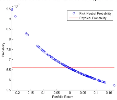
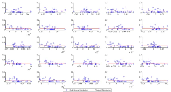
Figure 1 illustrate this property when we take γ = −3 and use the 25 Fama and French size and book to market portfolios. Notice that in this figure we plot on the “x” axis the return on the portfolio, endogenously chosen, hold by the representative agent while in the “y” axis the figure plots the respective risk neutral and physical distributions. Unfortunately the hyperbolic structure for the risk neutral distribution only holds for the endogenous portfolio, not for the individual assets itself. Figure 2 plot, for a selected date, the generated risk neutral distribution for the 25 Fama and French size and book to market portfolios used as basis assets. As it is clear the distortion generated by the risk neutral distribution is not uniform across assets. Nonetheless it is also noticeable
11For example in VaR estimations.
12The derivative signal of this function will depend on the Lagrange multipliers that will determine if the agent is long of short in the portfolio.
13
Physical and Risk Neutral Probabilities: Endogenous Portfolio
Figure 1: This figure presents the physical and implied risk neutral probabilities. In this example e set as our basis assets the 25 Fama and French equally weighted size and book to market portfolios and considered a 200 days time span. γ =−3.
that risk neutral probabilities can substantially differ from physical ones, specially for tail returns.
Given the methodology to estimate the pricing kernel previously discussed, we can proceed to the calculation of our tail risk measure14
. As discussed in the introduction, despite the fact that we do not rely on option data availability to calculate our measure, we still rely on the fact that prices of deeply out of the money puts contain information about future downturns. Thus, keeping this feature in mind, we set our main tail risk measure as the average price of a out of the money synthetic put for the basis assets in the estimation procedure:
P = T X
i=1
πi[max(K−R,0)] (8)
Where K is the, risk neutral, strike.
One question that might come to the readers mind is why to construct a tail risk mea-sure based on firms or portfolios rather then a market tail risk meamea-sure? Bali et al. (2013)
14
Physical and Risk Neutral Probabilities: Individual Fama French Portfolios
Figure 2: This figure presents the physical and implied risk neutral probabilities for a selected date setting γ =−3, the 25 Fama and French equally weighted size and book to market portfolios as our basis assets and 30 days in the estimation procedure.
argues that previous studies showed that investors usually holds a portfolios composed usually by some market proxy (e.g. stock funds) and individual stocks. When considering this kind of portfolio individual stocks play a crucial role on the total portfolio tail risk. Also, they find evidence that market tail risk is not capable of providing useful informa-tion for return predicinforma-tion whereas individual assets tail risk measures (idiosyncratic tail risk) is quite successful in predicting market returns.
3.1
Asset Pricing Models: Minimum Distance Problem
In the previous section we described a completely non parametric procedure to esti-mate the stochastic discount factor used to generate our tail risk measure. In this section we discuss a similar approach, presented by (Almeida and Garcia, 2012), that allows us to reconcile the previous methodology with asset pricing models implied SDF’s.
Bali et al. (2013) highlighted that some of the recent economic literature treated return in a asymmetric way, giving different weights to higher or lower returns, a feature that is of particular interest here. As previously presented one of the branches that considered this approach is the Rietz-Barro’s like models which incorporate the possibility of disaster in consumption to connect Mehra and Prescott (1985) results with a more structured macroeconomic model. Another venue in the literature started by Routledge and Zin (2010) and also studied by Bonomo et al. (2011) focus on generalized disappointment aversion preferences as a possible explanation for the equity premium puzzle. In the same spirit as Barro but with a different view of tail events, the disappointment aversion literature models “bad” outcomes in consumption directly in the agents utility function. The main idea behind this literature is that when negative outcomes occur the agents utility function suffer a negative shock leading to a volatile risk aversion over time and providing a very good match with real data.
Even more interestingly, by using the generalized disappoint aversion utility function the representative agent maximization problem implies a stochastic discount factor ex-plicitly dependent on tail events. For instance, if outcomes are above some threshold (generally a fraction of the certain equivalent), the stochastic discount factor falls into the usual Epstein-Zin formula. On the other hand, when tail events happen, the SDF formula changes, with agents giving more weight to relatively “bad” states of nature. This formulation is also very insightful for our tail risk approach, since it provides us with a clear intuition and interpretation.
δM D = min
m∈L2 E[φ(1 +m−y(θ)]
subject to E[m(R− 1
a1K)] = 0K m >0
(9)
Using the same dual problem technology applied in the last section Almeida and Garcia (2012) showed that15
under the Cressie-Read family of discrepancy functions the closest admissible SDF to the asset pricing model y(θ) is given by:
m(θ) =y(θ)−1 + (γλ′∗x) 1
γ (10)
Where λ′
∗ is the solution of equation (9) dual problem. Thus, given any asset pricing
model of interest this methodology allow us to empirically search for a semi-parametric SDF that correctly prices a chosen set of basis assets and satisfy non arbitrage conditions as in the previous section. The biggest difference however relies on the fact that this semi-parametric SDF depends on the choice of the asset pricing model.
Notably however, independent of the models choice, the implied pricing kernel will always inherit the interesting property that probabilities will be distorted to give more weight to “bad” outcomes. Aiming to capture this particular characteristic, and since the main focus of this present paper is not asset pricing models SDF estimation, in the empirical section we proceed with the non parametric approach.
4
Empirical Results
4.1
The Data
Throughout the paper we make use of several data sets. To keep things organized we summarize all the data used in table 1.
Starting with the calculation of our tail risk measure we must choose the basis assets to our non parametric SDF’s estimation. Aiming to eliminate some idiosyncratic effects but to still consider cross section information we set the 25 Fama and French size and book to market value weighted portfolios from Kenneth French library 16 as our basis
15
See theorem 1 of their paper. 16
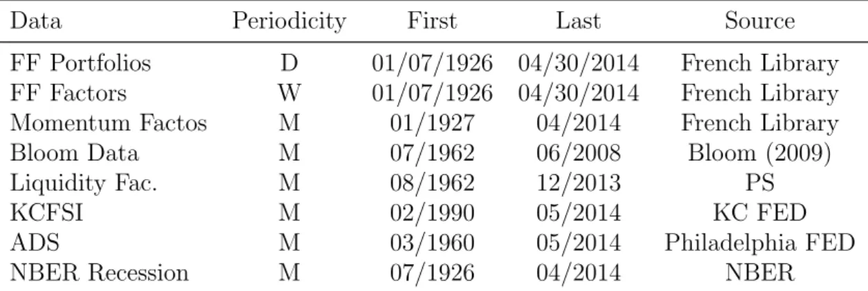
Table 1: The Data
Data Periodicity First Last Source
FF Portfolios D 01/07/1926 04/30/2014 French Library FF Factors W 01/07/1926 04/30/2014 French Library Momentum Factos M 01/1927 04/2014 French Library
Bloom Data M 07/1962 06/2008 Bloom (2009)
Liquidity Fac. M 08/1962 12/2013 PS
KCFSI M 02/1990 05/2014 KC FED
ADS M 03/1960 05/2014 Philadelphia FED
NBER Recession M 07/1926 04/2014 NBER
The first column indicates the data itself while the following columns indicate the periodicity, first and last observation date and source respectively. D, W, M, Q indicates daily, weekly, monthly and quarterly data respectively. ADS stands for Aruoba-Diebold-Scotti Business Conditions Index, KCFSI for Kansas City Financial Stress Index and PS for Pastor and Stambaugh (2003).
assets for the estimation procedure.
In the stock market section we use data from French library for the three Fama and French factors and momentum factors and data for the liquidity factor from Pastor and Stambaugh (2003). For macroeconomic activity indicators variables we consider a variety of sources: NBER recession dummy, Kansas City and Philadelphia FED. When discussing the uncertainty channel approach we rely on data from Bloom (2009). For spread pre-diction regressions bond data was collected from Saint Louis FED FRED database.
4.2
Empirical Features
Given our preliminary choice we can now focus on the relation of our tail risk measure with market returns. Considering the CRSP market index as a proxy for the later, table 2 presents the correlation coefficients between our tail risk measure and the index return. As expected our measure is highly counter cyclical, whenever market is more bullish our tail risk measure is small. On the other hand, when market is more bearish our tail risk measure is high. 17
Table 2: Tail Risk Correlations
CRSP V IX2 KJ BTX CATFIN TSM Bloom
Tail Risk -0.3549 0.4094 0.0327 0.2837 0.3800 0.2452 0.2240 This table present the correlation coefficient between our tail risk mea-sures and CRSP market index,V IX2
index, Kelly and Jiang (2013) (KJ) and Bollerslev et al. (2014) (BTX) tail risk measures, CATFIN measure from (Allen et al., 2012), Bali et al. (2014) (TSM) macroeconomic risk index and Bloom (2009) uncertainty index. All correlations are contem-poraneous.
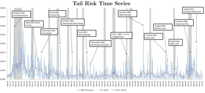
To give a better view of what is going on, figure 3 plots the evolution of our tail risk measure, in blue, and Hoddrick-Prescott trend, in red, when we use a monthly time span (30 days) in the estimation from July 1926 to April 2014. Prominently our measure is very volatile and present various peeks, in accordance with Bollerslev et al. (2014) proposed measure. Indeed table 2 also revealed that our tail risk measure is relatively correlated with Bollerslev et al. (2014) one.
Still considering figure 3 we highlighted dates that represents huge markets falls in the U.S. history. Interestingly the tail risk measure peaks in most of this events and also appears to be more volatile in the periods before and after some of them. Another compelling feature is the measure volatility during 1929 recession period and WWII. Even more striking is the fact that the measure trend, red line, increased both before 1929 and 2008 crisis. Motivated by this superficial result we further explore our tail risk measure relationship with market variables in section 4.3 and seek business cycles analysis in section 4.4.
Closing up this section we provided a heuristic discussion between our tail risk mea-sure, the V IX2
index, Kelly and Jiang (2013) and Allen et al. (2012) tail risk measures.
17
Tail Risk Time Series
Figure 3: This figure presents the Tail Risk (TR) time evolution from July 1926 to April 2014. Blue line indicate the actual tail risk series while red line indicate Hoddrick-Prescott filtered trend. Tail Risk was calculated using 25 Fama and French equally weighted size and book to market portfolios as basis assets considering a time span of one month (30 days) and γ =−3.
First, observe that the V IX2 is based on a risk neutral probability whereas conditional
variance uses the physical probability (Bekaert and Hoerova, 2013). Thus, theV IX2
in-dex actually captures jump process (distastes risks) since the diffusion term remains the same under risk neutral or physical probabilities ((Bollerslev et al., 2014)). Given that, our tail risk measure has a close relationship with the VIX index since, as put by Bekaert and Hoerova (2013), the index reflects “risk neutral” expected stock market variance for S&P 500.
Further looking into this fact, table 2 present the correlation between the V IX2
and tail risk, which confirms our expectation. Taking a close look at figure 3 we note that the tail risk measure peaks, as the V IX2
, in October 2008 and appears to return to a pre crises level more smoothly them the V IX2. This is not true however for the 2010
European debt crisis where both the measure and the index appear to revert to the mean quite quickly. This mean reversion is also noted to other crisis in the 1990 - 2014 period highlighted in figure 3. Since our measure is significantly correlated with the VIX index we believe that in some extent we are actually capturing some portion of the variance risk premium.
this result is due to the intrinsic characteristic of both measures. For instance while Kelly and Jiang measure is based on a parametric hypothesis for the returns left tail distribution our tail risk consists on financial measures based on the risk neutral distribution. Also, Kelly and Jiang tail risk present a very persistent auto-regressive coefficient, a very nice feature for long term prediction while the respective result four our measure is 0.4321, much smaller.
Finally, as table 2 revels, the closes measure to ours is (Allen et al., 2012) CATFIN measure. In fact (Allen et al., 2012) financial distress measure is calculated via a Value at Risk approach for financial institutions. In some sense our measure is intrinsic related to theirs given that we also look for events that are on the left side or the returns distribution. On the other hand, while they just consider say the first decile (under the physical probabilities) of the return distribution, our measure averages all returns below some threshold using risk neutral information.
4.3
Stock Markets Returns
While the previous section discussed generic properties of out tail risk measure, this section investigates whether of not expected returns are related to a tail risk factor.
For notation purposes let Ri
t denote asset i return at time t and Ft a K ×1 vector of possible factors, except tail risk, that explain the assets returns. To perform our empirical analysis we select the following sets of factors as controls: the three Fama and French (1988) factors, the momentum factor and a liquidity factor proposed by Pastor and Stambaugh (2003).
As in Kelly and Jiang (2013) our working hypothesis is that investors marginal utility is increasing with tail risk, in line with the counter-cyclical property observable in figure 3. In other words, investors are averse to tail risk, and thus assets that hedge this source of risk are expected to have lower future returns. On the other hand assets that are highly exposed to tail risk are expected to have higher future returns.
The methodology consists in sorting assets, here taken to be the NYSE/AMEX/NASDAQ stocks with CRSP share codes 10 and 11, into portfolios depending on their sensitivity to tail risk. That sensitivity consists in the ordinary least square coefficient γi
Ri t−R
f
t =αit+γtiT Rt+ǫt (11) At the end of each month in our data set18
we select the previous 10 years data and proceed to the estimation of regression (11). After the estimation we select the estimated γi and sort the assets into five quintiles based on their tail risk sensitivity. We than track each assets return one month and one year ahead after the sorting. This implies that the tracked returns are truly out of the sample since we only condition the sorting on data available until date t.
The second step of this procedure consist in estimating regression 12 and computing the respective α′s. If the estimated value for α is different from zero this is evidence that
our factor explains a component of expected returns not captured by con control factors Ft.
˜
Rt =αit+β i
tFt+ǫt (12)
By proceeding in this venue the estimated coefficient γi
t capture the co-movements of expected returns, for each assets, with tail risk. Notice also that due to the rolling window adopted in the estimation procedure we allow γi
t to vary across periods, implicating that assets can change quintiles whenever we sort the portfolios.
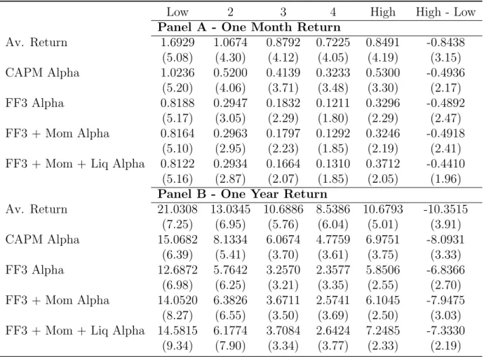
Table 3 reports the final result for this procedure. First line of each panel present the portfolios returns for one month and one year holding period (after the sorting). Subsequent lines present the alphas from regressions considering four factor models spec-ifications: CAPM, Fama and French three factor model, a Four Factor model that con-trols for momentum factor and a additional Five Factor model that considers Pastor and Stambaugh (2003) liquidity factor.
Analyzing results in table 3 we can note that for both one month and one year holding period portfolios with returns that co-vary positively with tail risk (and thus work as a hedge to tail risk) have smaller returns than portfolios with smaller or negative correlation with tail risk (Low column). In fact, the last column of each panel reveals that for one month and one year holding period this difference is 0.8438% and 10.3515% respective, with both values been statistically significant at 1% significance level.
18
Table 3: Tail Risk Beta-Sorted Portfolios: Endogenous Put
Low 2 3 4 High High - Low
Panel A - One Month Return
Av. Return 1.6929 1.0674 0.8792 0.7225 0.8491 -0.8438 (5.08) (4.30) (4.12) (4.05) (4.19) (3.15) CAPM Alpha 1.0236 0.5200 0.4139 0.3233 0.5300 -0.4936
(5.20) (4.06) (3.71) (3.48) (3.30) (2.17) FF3 Alpha 0.8188 0.2947 0.1832 0.1211 0.3296 -0.4892
(5.17) (3.05) (2.29) (1.80) (2.29) (2.47) FF3 + Mom Alpha 0.8164 0.2963 0.1797 0.1292 0.3246 -0.4918
(5.10) (2.95) (2.23) (1.85) (2.19) (2.41) FF3 + Mom + Liq Alpha 0.8122 0.2934 0.1664 0.1310 0.3712 -0.4410
(5.16) (2.87) (2.07) (1.85) (2.05) (1.96) Panel B - One Year Return
Av. Return 21.0308 13.0345 10.6886 8.5386 10.6793 -10.3515 (7.25) (6.95) (5.76) (6.04) (5.01) (3.91) CAPM Alpha 15.0682 8.1334 6.0674 4.7759 6.9751 -8.0931
(6.39) (5.41) (3.70) (3.61) (3.75) (3.33) FF3 Alpha 12.6872 5.7642 3.2570 2.3577 5.8506 -6.8366
(6.98) (6.25) (3.21) (3.35) (2.55) (2.70) FF3 + Mom Alpha 14.0520 6.3826 3.6711 2.5741 6.1045 -7.9475
(8.27) (6.55) (3.50) (3.69) (2.50) (3.03) FF3 + Mom + Liq Alpha 14.5815 6.1774 3.7084 2.6424 7.2485 -7.3330
As it can also be noted, results in for the estimated α′s for both one month and one
year ahead High minus Low portfolios returns are negative, and statistically significant, for all the specifications considered.
4.4
Economic Predictability
While the previous section of the paper focused on tail risk implication for stock market returns the remainder of the paper explores tail risk relationship with real economy through the uncertainty channel. Relying on this argument, and also discussing additional properties of our tail risk measure, we present several prediction results for macroeconomic and firm level variables.
Bloom (2009) seminal paper argued that economic uncertainty impacts firms invest-ment decision, often postponing investinvest-ment and reducing employinvest-ment. In fact, as high-lighted by Kelly and Jiang (2013), Bloom analysis can be related to tail risk, since as we already discussed in the introduction there is a close relationship between uncertainty and tail risks. For instance table 2 reveals that indeed our tail risk measure is significantly correlated with V IX2
index and both Bloom’s and Bali et al. uncertainty measures. This feature is even more striking when comparing the different methodologies adopted to estimate our tail risk measure in contrast with Bloom’s and Bali et al. ones.
In his paper, Bloom verified that stock market volatility presented a certain kind of “jump” in some occasions (mostly the ones highlighted in figure 3). To access whether this volatility shocks influence firm level decision, as a first step, Bloom proposed a vector auto-regressive impulse response function approach to motivate his model.19
. By using a his proxy for uncertainty, Bloom found that both industrial production and employment reduces in the short run whenever uncertainty raises. We argue that some of the uncertainty effect captured by Bloom’s study might actually be coming from tail risk, in the same line as Kelly and Jiang (2013), but relying in a more heuristic approach. The main idea behind our argument is similar to that explored by Kellogg (2010) who argued that rises in volatility, in our case tail risks, are associated with rises in firms real options.20
19Bloom considered the following variables in the VAR approach: industrial production in manufac-turing, employment in manufacmanufac-turing, hours in manufacmanufac-turing, CPI, wages, federal found rates, stock market level (measures by S&P 500 index), and a volatility uncertainty indicator
20
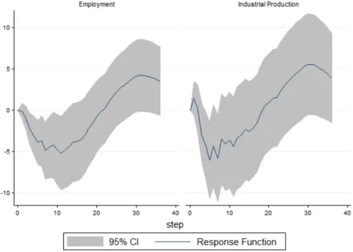
To test this hypothesis we follow Bloom’s vector auto-regressive approach and eval-uated the impulse response function on both employment and industrial production to a shock in tail risk. Using Hodrick-Prescott filter we detrended all variables used in the VAR regression21
. Figure 4 plot the impulse response function for one standard deviation shock in the monthly estimated tail risk measure22. The gray area represents the 95%
confidence interval for the response function while the solid line represent the response itself. Our results are quite similar to those found by both Bloom (2009) and Kelly and Jiang (2013) with response functions presenting a rapid drop in both the industrial pro-duction and employment in the manufacturing sector after the tail risk shock within 10 and 4 months for employment industrial production respectively. Still in line with their results, we observe a similar dynamics in post shock periods.
Employment and Industrial Production Impulse Response
Figure 4: This figure presents the impulse response function on Employment and In-dustrial Production (for the manufacturer sector) based on a VAR estimation (Bloom (2009)). The impulse response functions are relative to one standard deviation shock on tail risk.
Still pursuing this line of argument we believe that one of the key variables consid-ered by managers are the yield spread. Rises in the spread are usually associated with
21
As Bloom we setλ= 129,600. 22
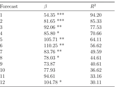
Table 4: Spread prediction
Forecast β R2
1 54.35 *** 94.20
2 81.65 *** 85.33
3 92.06 ** 77.53
4 85.80 * 70.66
5 105.71 ** 64.11
6 110.25 ** 56.62
7 83.76 ** 49.59
8 78.03 * 44.61
9 73.87 40.61
10 77.93 36.62
11 94.61 33.16
12 104.78 * 30.11
* p <0.10, **p <0.05, ***p <0.01
This table present the prediction regressions for Yields spread. Spread is calculated by the differ-ence between BAA and AAA bonds. t-statistics are calculated using Newey and West (1987) vari-ance matrix.
macroeconomic uncertainty and investment postponement. The relationship of this vari-able with tail risk is thus relatively clear: whenever tail risk rises the probability of “bad” outcomes in the hole economy also rises. Paralleling disaster risks models, since this risk is embedded in the tail risk measure, a deterioration of the tail risk index might be a indicator of possible future defaults.
Spreadt+i =α+βT Rt+
11
X
k=0
γiSpreadt−k (13)
To verify our hypothesis that tail risk might be a good predictor of Yields spread e perform than a series of forecasting regressions. For each i = 1, . . . ,12 we estimate regression 13 and verify the estimated coefficient for tail risk, β. In line with our expec-tations, our forecasting regressions presented in table 4 indicated that a rise in the tail risk index implies that future spreads will, on average, be higher. Also, for most of the regression this coefficient turned out to be statistically significant with a reasonably high R2
statistics.
about future expectations.
4.4.1 Business Cycles
One important question behind previous section results is: does tail risk has any rela-tion with business cycles? The uncertainty channel argument already provided us some evidence that a raise in tail risk affect firms investment decision. To further clarify the argument, in figure 3 we plot our tail risk, in blue, and highlight the NBER recession periods. To give a better idea of tail risk and recessions relation we also plot in red the same tail risk measure 23 but now Hoddrick Prescott filtered. Interestingly the
rela-tion between the measure and bussiness cycles becomes much more clear, revealing that usually tail risk is higher whenever the economy is in a recession.
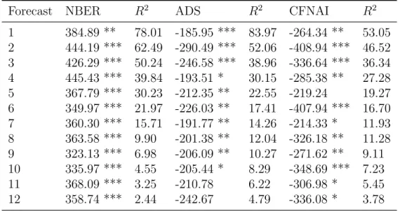
Given that, since our tail risk measure is based on cross section pool of firms we ask whether the systematic risk capture by the measure has any predictability over economic downturns. Our approach is comparable to Allen et al. (2012) who consider systemic risk for the financial sector as predictors for economic downturns. Their argument is that financial industry are “special” to the economy since they provide the intermediation link between investors. Differently from their paper however we argue that real economy systemic tail risk also play a important role on stress macroeconomic variables prediction. Following Allen, Bali and Tang we choose a variety of macroeconomic indicators for prediction regressions: The Kansas City FED Financial Stress Index, the Arouba-Diebold-Scott (ADS) Bussiness Conditions Index and finally NBER recession indicators to illustrate our argument. We highlight that Kansas City FED and NBER Recession indicator are counter cyclical while ADS index is pro cyclical. Consider then the following regression:
It+i =β0+βT Rt+ 11
X
k=0
γiIt−k+ǫt (14)
WhereI stands for the four possible indexes we consider andiindicate the forecasting period (i= 1, . . . ,12). Note that since NBER recession indicator is a binary variable we estimate the regression using Probit technique instead of standard OLS.
A first glimpse in table 5, which present the results for the regressions, reveal that the indeed tail risk is capable to anticipate these macroeconomic indicators with
reason-23
Table 5: Macroeconomic Indicator Regressions Forecast NBER R2
ADS R2
CFNAI R2
1 384.89 ** 78.01 -185.95 *** 83.97 -264.34 ** 53.05 2 444.19 *** 62.49 -290.49 *** 52.06 -408.94 *** 46.52 3 426.29 *** 50.24 -246.58 *** 38.96 -336.64 *** 36.34 4 445.43 *** 39.84 -193.51 * 30.15 -285.38 ** 27.28 5 367.79 *** 30.23 -212.35 ** 22.55 -219.24 19.27 6 349.97 *** 21.97 -226.03 ** 17.41 -407.94 *** 16.70 7 360.30 *** 15.71 -191.77 ** 14.26 -214.33 * 11.93 8 363.58 *** 9.90 -201.38 ** 12.04 -326.18 ** 11.28 9 323.13 *** 6.98 -206.09 ** 10.27 -271.62 ** 9.11 10 335.97 *** 4.55 -205.44 * 8.29 -348.69 *** 7.23 11 368.09 *** 3.25 -210.78 6.22 -306.98 * 5.45 12 358.74 *** 2.44 -242.67 4.79 -336.08 * 3.78 * p <0.10, **p <0.05, *** p <0.01
Entries represent the tail risk coefficient for prediction regressions. Lines indicate the predicted horizon. t-statistics are calculated using Newey and West (1987) variance matrix.
able performance. For instance, a couple features are noted: the coefficients for NBER recession indicators is positive, with one exception, while the respective values for ADS and CFNAI indicators are negative. That is, whenever tail risk increases at time t on average there is a economic deceleration in the future. The second feature we note is that when we increase i the net effect of a increase in tail risk appears to decreases for all macroeconomics activities index considered, with a clear trend to the NBER recession indicator.
5
Conclusion
In this paper we introduce a novel procedure to gauge tail risk, i.e. the risk of economic crises. The approach can be split in three steps. First, we extract risk neutral probabilities from a set of basis assets, in this paper chosen to be the 25 Fama-French portfolios sorted by size and book-to market values. From the risk neutral distribution we calculate the price of a synthetic put and set it as our tail risk measure. Due to it’s independence of option data availability our methodology allow us to estimate a long series, dating back to 1926.
hypothesis and economic prediction. With respect to the cross section of returns our factor presented negative, statistically significant, α′s for one year ahead excess returns
on portfolios sorted by tail risk sensitivity.
Macroeconomic activity index prediction regressions revealed that our tail risk index is able to anticipate their movements. When analyzing firm level decisions we found that raises in tail risks influences negatively short term industrial production and employment and also predicts future yield spreads.
From an academic point of view, our findings corroborated with previous studies in the tail risk literature and provide a new methodology that is applicable to virtually all markets where assets are traded. From a practical standpoint, we offer a useful tool for managers and regulators to control the exposure of portfolios and institutions to extreme events.
References
Ait-Sahalia, Y. and A. W. Lo (1998, 04). Nonparametric Estimation of State-Price Densities Implicit in Financial Asset Prices. Journal of Finance 53(2), 499–547.
Ait Sahalia, Y. and A. W. Lo (2000). Nonparametric risk management and implied risk aversion. Journal of Econometrics 94(1-2), 9–51.
Allen, L., T. G. Bali, and Y. Tang (2012). Does systemic risk in the financial sector predict future economic downturns? Review of Financial Studies 25(10), 3000–3036.
Almeida, C. and R. Garcia (2012). Assessing misspecified asset pricing models with empirical likelihood estimators. Journal of Econometrics 170, 519–537.
Almeida, C. and R. Garcia (2014). Economic implications of nonlinear pricing kernels.
Bali, T. G., S. J. Brown, and M. O. Caglayan (2014). Macroeconomic risk and hedge fund returns. Journal of Financial Economics 114(1), 1 – 19.
Bali, T. G., N. Cakici, and R. F. Whitelaw (2013, September). Hybrid tail risk and expected stock returns: When does the tail wag the dog? Working Paper 19460, National Bureau of Economic Research.
Barro, R. J. (2009, March). Rare Disasters, Asset Prices, and Welfare Costs. American
Economic Review 99(1), 243–64.
Bates, D. S. (1991, July). The Crash of ’87: Was It Expected? The Evidence from Options Markets. Journal of Finance 46(3), 1009–44.
Bekaert, G. and M. Hoerova (2013, April). The VIX, the Variance Premium and Stock Market Volatility. NBER Working Papers 18995, National Bureau of Economic Re-search, Inc.
Bloom, N. (2009, 05). The Impact of Uncertainty Shocks. Econometrica 77(3), 623–685.
Bollerslev, T. and V. Todorov (2011, December). Tails, Fears, and Risk Premia. Journal
of Finance 66(6), 2165–2211.
Bollerslev, T., V. Todorov, and L. Xu (2014, May). Tail risk premia and return pre-dictability. Technical report.
Bonomo, M., R. Garcia, N. Meddahi, and R. T´edongap (2011). Generalized Disap-pointment Aversion, Long-run Volatility Risk, and Asset Prices. Review of Financial Studies 24(1), 82–122.
Borovicka, J., L. P. Hansen, and J. A. Scheinkman (2014, June). Misspecified Recovery. NBER Working Papers 20209, National Bureau of Economic Research, Inc.
Breeden, D. T. and R. H. Litzenberger (1978, October). Prices of State-contingent Claims Implicit in Option Prices. The Journal of Business 51(4), 621–51.
Fama, E. F. and K. R. French (1988, October). Dividend yields and expected stock returns. Journal of Financial Economics 22(1), 3–25.
Jurado, K., S. C. Ludvigson, and S. Ng (2013, September). Measuring Uncertainty. NBER Working Papers 19456, National Bureau of Economic Research, Inc.
Kellogg, R. (2010, November). The effect of uncertainty on investment: Evidence from texas oil drilling. Working Paper 16541, National Bureau of Economic Research.
Kelly, B. and H. Jiang (2013, August). Tail risk and asset prices. Working Paper 19375, National Bureau of Economic Research.
Longstaff, F. A. (1995). Option Pricing and the Martingale Restriction. Review of Financial Studies 8(4), 1091–1124.
Markowitz, H. (1952, 03). Portfolio Selection. Journal of Finance 7(1), 77–91.
Mehra, R. and E. C. Prescott (1985, March). The equity premium: A puzzle. Journal of
Monetary Economics 15(2), 145–161.
Newey, W. K. and K. D. West (1987, May). A Simple, Positive Semi-definite, Heteroskedasticity and Autocorrelation Consistent Covariance Matrix. Economet-rica 55(3), 703–08.
Pastor, L. and R. F. Stambaugh (2003, June). Liquidity Risk and Expected Stock Re-turns. Journal of Political Economy 111(3), 642–685.
Paul Glasserman, Chulmin Kang, W. K. (2013, April). Stress scenario selection by empirical likelihood. Technical report, Office of Financial Research.
Perotti, E., L. Ratnovski, and R. Vlahu (2011, August). Capital Regulation and Tail Risk. DNB Working Papers 307, Netherlands Central Bank, Research Department.
Ross, S. A. (2011, August). The recovery theorem. Working Paper 17323, National Bureau of Economic Research.
Routledge, B. R. and S. E. Zin (2010, 08). Generalized Disappointment Aversion and Asset Prices. Journal of Finance 65(4), 1303–1332.
Rubinstein, M. (1994). Implied binomial trees. Journal of Finance 49(3), 771–818.
Siriwardane, E. (2013). The probability of rare disasters: Estimation and implications. Technical report, NYU Stern School of Business.
Snow, K. (1991). Diagnosing asset pricing models using the distribution of assets returns.
Journal of Finance (46), 955–883.
Stutzer, M. (1996). A simple nonparametric approach to derivative security valuation.
Journal of Finance 51(5), 1633–52.
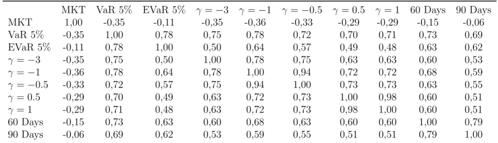
Table 6: Correlations Between Tail Risk Measures
MKT VaR 5% EVaR 5% γ =−3 γ =−1 γ =−0.5 γ = 0.5 γ = 1 60 Days 90 Days MKT 1,00 -0,35 -0,11 -0,35 -0,36 -0,33 -0,29 -0,29 -0,15 -0,06 VaR 5% -0,35 1,00 0,78 0,75 0,78 0,72 0,70 0,71 0,73 0,69 EVaR 5% -0,11 0,78 1,00 0,50 0,64 0,57 0,49 0,48 0,63 0,62
γ =−3 -0,35 0,75 0,50 1,00 0,78 0,75 0,63 0,63 0,60 0,53
γ =−1 -0,36 0,78 0,64 0,78 1,00 0,94 0,72 0,72 0,68 0,59
γ =−0.5 -0,33 0,72 0,57 0,75 0,94 1,00 0,73 0,73 0,63 0,55
γ = 0.5 -0,29 0,70 0,49 0,63 0,72 0,73 1,00 0,98 0,60 0,51
γ = 1 -0,29 0,71 0,48 0,63 0,72 0,73 0,98 1,00 0,60 0,51 60 Days -0,15 0,73 0,63 0,60 0,68 0,63 0,60 0,60 1,00 0,79 90 Days -0,06 0,69 0,62 0,53 0,59 0,55 0,51 0,51 0,79 1,00
This table present the correlations coefficients between estimated tail risk measure when considering alter-native specifications. For the baseline case, γ =−3, we estimate tail risk using the 25 Fama and French size and book to market sorted portfolios and a 30 days time span. Possible variations of the baseline case are indicated in the lines/columns.
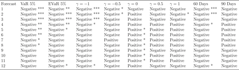
Table 7: Robustness ADS
Forecast VaR 5% EVaR 5% γ =−1 γ =−0.5 γ = 0 γ = 0.5 γ = 1 60 Days 90 Days 1 Negative *** Negative ** Negative *** Negative * Negative Negative Negative Negative *** Negative 2 Negative *** Negative *** Negative *** Negative * Positive Negative Negative * Negative *** Negative 3 Negative *** Negative *** Negative *** Negative Positive Negative Negative Negative Negative 4 Negative ** Negative ** Negative * Negative Positive Positive Positive Negative * Positive 5 Negative ** Negative * Negative Negative Positive * Positive Positive Negative Positive 6 Negative ** Negative Negative Negative Positive * Positive Positive Negative Positive 7 Negative * Negative Negative Positive Positive * Positive Positive Negative Positive 8 Negative * Negative Negative Negative Positive * Positive Positive Negative Positive 9 Negative Negative Negative Negative Positive * Negative Negative Negative Negative 10 Negative Negative Negative Negative Positive * Positive Positive Negative Negative 11 Negative Negative Negative Negative Positive * Positive Positive Negative Negative 12 Negative Negative * Negative * Negative Positive Negative Negative Negative * Negative
This table present the robustness tests for ADS.
Table 8: Robustness CFNAI
Forecast VaR 5% EVaR 5% γ =−1 γ =−0.5 γ = 0 γ = 0.5 γ = 1 60 Days 90 Days 1 Negative *** Negative ** Negative ** Negative ** Negative Negative * Negative * Negative *** Negative ** 2 Negative *** Negative *** Negative ** Negative Negative Negative Negative * Negative *** Negative 3 Negative *** Negative ** Negative *** Negative ** Positive * Negative Negative Negative * Negative 4 Negative ** Negative * Negative * Negative Positive Positive Negative Negative * Positive 5 Negative * Negative ** Negative * Negative Positive * Negative Positive Negative ** Positive 6 Negative ** Negative * Negative ** Negative Positive Positive Positive Negative Positive 7 Negative * Negative Negative Negative Positive * Positive Positive Negative * Positive 8 Negative Negative Negative Positive Positive Positive Positive Negative Positive 9 Negative ** Negative Negative * Negative Positive * Negative Negative Negative * Negative 10 Negative * Negative Negative * Negative Positive Negative Negative Negative Negative 11 Negative Negative Negative Negative Positive * Positive Positive Negative Negative 12 Negative * Negative ** Negative ** Negative Positive Negative Negative Negative * Negative
This table present the robustness tests for CFNAI.