CRISTIANO FIORILO DE MELO AND OTHON CABO WINTER Received 28 December 2004; Revised 27 July 2005; Accepted 23 August 2005
The planar, circular, restricted three-body problem predicts the existence of periodic or-bits around the Lagrangian equilibrium point L1. Considering the Earth-lunar-probe sys-tem, some of these orbits pass very close to the surfaces of the Earth and the Moon. These characteristics make it possible for these orbits, in spite of their instability, to be used in transfer maneuvers between Earth and lunar parking orbits. The main goal of this paper is to explore this scenario, adopting a more complex and realistic dynamical system, the four-body problem Sun-Earth-Moon-probe. We defined and investigated a set of paths, derived from the orbits around L1, which are capable of achieving transfer between low-altitude Earth (LEO) and lunar orbits, including high-inclination lunar orbits, at a low cost and with flight time between 13 and 15 days.
Copyright © 2006 C. F. de Melo and O. C. Winter. This is an open access article distrib-uted under the Creative Commons Attribution License, which permits unrestricted use, distribution, and reproduction in any medium, provided the original work is properly cited.
1. Introduction
Ever since the beginning of space exploration, the Moon has been the target of countless missions, and everything leads to believe that this will continue to be so. This certainty is focused on the recent discoveries of signs that point to the possible existence of ice at the lunar poles made by the American probes Clementine in 1994 [21] and Lunar Prospector in 1998 [10]. The estimates indicate that there may be some 10 billion tons of ice at the lunar poles. Therefore, if the existence of this ice were confirmed, future lunar bases would have a water source capable of sustaining life. This ice could also serve as a source for rocket fuel, by separating the water into hydrogen and oxygen, thus making the Moon into a trampoline for future manned interplanetary missions.
In this context, a special type of path, capable of direct transfer between a low-altitude Earth orbit (LEO) and a low-altitude Moon orbit, with flight time between 13 and 15 days, could be of great interest for future lunar missions. This paper presents the results
of our research on this type of path, and shows that these paths could be a good alterna-tive for an Earth-Moon transfer, and also other kinds of transfer in Earth-Moon system. The origin of these paths is related to a family of generally unstable direct orbits around the Lagrangian equilibrium point L1, known as the Family G. These paths are predicted by the circular, planar, restricted three-body problem associated with the Earth-Moon system (Broucke [8]). This is why we initially considered the three-body Earth-Moon-probe problem to establish a set of initial conditions, close to the Earth, and final con-ditions, close to the Moon, in such a way that these conditions were related through an empirical mathematical expression. Next, we considered a more complex and realistic dynamical problem, the four-body problem Sun-Earth-Moon-probe, where we take into account the eccentricity of the Earth’s orbit as well as the eccentricity and inclination of the Moon’s orbit. An empirical expression related to the initial and final conditions of the paths continued to exist. On the other hand, the consideration of a more complex dynam-ical system opened up new lines of investigation with respect to the probe’s inclination and speed on its final approach to the Moon.
This paper is structured as follows. In Section 2, to facilitate comparison, we have quickly described two of the main conventional methods of Earth-Moon transfer and the method of gravitational capture. InSection 3, we describe the two dynamical sys-tems utilized in this study. InSection 4, we discuss the main properties of these orbits for the restricted three-body problem and the four-body problem. InSection 5, we present, through a curve and an empirical mathematical expression, the set of paths capable of making the maneuver. In Section 6, we present some examples of missions that could be made using these paths, and finally, inSection 7, we present our conclusions and the perspective for future researches.
2. Conventional methods of Earth-Moon transfers
The calculation of a transfer path between the Earth and the Moon can only be made through numerical integration of the equations of motion [1]. These equations must take into account the Earth’s, Moon’s, and Sun’s gravitational fields, and the mutual interac-tions between these bodies. In addition, given the complexity of the Moon’s movement, a lunar mission must be planned and executed on an hour-by-hour and day-by-day basis. However, we can consider some approximations, based on the two-body and restricted three-body problem, to reach an initial estimate of the impulse needed to transfer a probe from the vicinity of the Earth to the vicinity of the Moon.
Next, we will describe two conventional methods used for preliminary analysis of the
∆V’s necessary for an Earth-Moon transfer and the gravitational capture method. Our goal is not to describe them rigorously, but rather to create a basis for comparison with the transfers that could be done by a set of paths derived from the unstable orbits around the Lagrangian equilibrium point L1; a set that we will present inSection 5.
∆V1 VE1 V1
1 2
R1
Earth
Earth’s parking orbit
D R2
D
R2
Moon Moon’s parking
orbit Moon’s orbit
Transfer ellipse (minimal energy path)
Moon at the instant of injection of probe in transfer ellipse
(a)
VE2 R2
VMoon
Moon
Lunar parking orbit
(b)
∆V2 VL2
V2 R2
Moon Lunar parking
orbit
(c)
Figure 2.1. (a) Minimal energy transfer ellipse and the Earth’s and Moon’s circular parking orbits in geocentric system. (b) Velocities of the Moon and of the probe (in its apogee’s transfer ellipse) in geocentric system. (c) Velocities of the probe relative to the Moon at the moment of application of the
∆V2in selenocentric system. (Not to scale.)
neglected. This way, we can establish a simple procedure to estimate the impulses required for the maneuver based on Hohmann’s transfer [1].Figure 2.1shows the minimal energy path, an ellipse, it is tangent to Earth’s and Moon’s parking orbits. The first part starts with the application of a∆V1when the vehicle attains the perigee’s transfer ellipse. From
Figure 2.1, we obtain the semimajor axis of transfer ellipse,amin, by
amin=R1+D −R2
2 , (2.1)
whereR1is the perigee’s radius of the transfer ellipse and also of the Earth’s parking orbit
radius in the point of tangency with the transfer ellipse,D=384 400 km is the
Earth-Moon distance which we are considering constant, that is, we are considering the Earth-Moon to be in a circular orbit around the Earth, andR2is the Moon’s parking orbit radius in
this ellipse is
ξmin= −GMEarth
2amin , (2.2)
whereG=6.67×10⁻¹¹m3/s2kg andM
Earth=5.9742×1024kg are the universal
gravita-tional constant and the mass of the Earth, respectively. Thus, we can obtain the perigee’s speed of the transfer ellipse,VE1, by
VE1=
2
GM
Earth
R1 +ξmin
(2.3)
and the apogee’s speed of transfer ellipse,VE2, by
VE2=
2
GM
Earth
D−R2
+ξmin
. (2.4)
If we consider that the Earth’s and Moon’s parking orbits are circular with radiusR1and
R2, respectively, the first impulse required to insert the vehicle in the transfer ellipse,∆V1,
is given by
∆V1=VE1−
GMEarth
R1
. (2.5)
As we can see, the first part of the maneuver is equal to Hohmann’s transfer. However, the second part of the maneuver corresponds to the application of a second impulse to insert the vehicle in lunar orbit and not to put it in a circular orbit with radiusD−R2.
Therefore, the second part is different from Hohmann’s transfer procedure, because the
∆V2required for this maneuver should be applied in the opposite direction of the vehicle’s
motion. In order to calculate the magnitude of∆V2, we should consider the apogee’s
vehicle speed,VE2, relative to the Moon. This speed we denote byVL2, and its magnitude
is given by
VL2=
VE2−VMoon
, (2.6)
whereVMoon=1.023 km/s is the Moon’s orbital speed around the Earth (assuming
circu-lar orbit). The magnitude of∆V2is immediately calculated by
∆V2=
GMMoon
R2
−VL2, (2.7)
whereMMoon=7.3483×10²²kg is the Moon’s mass, and
VE1 P
V1 ∆V1
φ1 R1
Earth’s parking orbit
Earth
D
Moon at the instant of injection of the probe
in the transfer ellipse Lunar sphere
of influence
D RI
I
Geocentric conic (ellipse)
Moon’s orbit Selenocentric
path (hyperbola)
Rs ∆V2 M λI
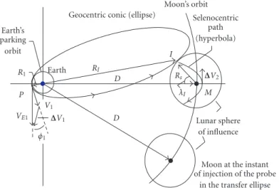
Figure 2.2. Geocentric conic of transfer (ellipse) and the transfer geometry seen in the geocentric coordinates system (not to scale).
The flight time for this maneuver is simply half of the orbital period of the transfer ellipse, that is,
TFlight=π
a3
min
GMEarth
. (2.9)
The procedure described in this section is the simplest method to estimate the mag-nitude∆VTotal for a direct maneuver transfer between the Earth and the Moon. But, it
makes use of two-body dynamics, for this reason, the∆VTotal given by (2.8) is not
suf-ficient to take the vehicle to the final lunar orbit desired, requiring additional∆V’s to complete the mission [18].
also shows the second part of the maneuver in which the probe gets inside the lunar sphere of influence.
The transfer starts when a∆V1is applied injecting the probe into geocentric conic, this
occurs at pointP(Figure 2.2). At the point at which the probe reaches the Moon’s sphere of influence, pointI (Figure 2.2), it begins to move under the influence of the Moon. When the probe reaches the periselenium of the selenocentric path, pointM(Figure 2.2), a∆V2must be applied to conclude the maneuver.
In order to calculate the elements of the geocentric and selenocentric paths and the
∆V’s required to transfer, we need to know at least four independent initial quantities, or three independent initial quantities and one intermediary (on the lunar sphere of influ-ence), or final quantities. The search for these quantities is an iterative procedure. Partic-ularly, a convenient set for these quantities isR1,VE1,φ1, andλI(seeFigure 2.2), where R1 is the radial distance at the point P,VE1is the injection speed into geocentric conic,
φ1is the flight-path angle, andλI specifies the point at which the geocentric trajectory crosses the lunar sphere of influence.
Thus, if the values attributed toR1,VE1,φ1, andλI lead the probe to periselenium equal to the radius of the final lunar orbit planed, the procedure is complete, otherwise, a new search for other values forR1,VE1,φ1, andλImust be started until the selenocentric path reaches periselenium equal to the radius of the final lunar orbit desired.
The procedure described above is a good approximation for preliminary mission anal-ysis, but, in practice, errors occur in the encounter with the Moon’s sphere of influence due to the disturbance of the Sun’s gravitational field, and also due to the Moon’s grav-itational field in the first part of the maneuver and the Earth’s in the second part of the maneuver. The calculations needed to reach the values of the∆V’s are extensive and for this reason, we will not demonstrate them here. For more information, please consult [1].
2.3. Methods of Earth-Moon transfer by gravitational capture. The phenomenon of gravitational capture can be understood as the mechanism by which an object, subject only to gravitational forces, approaches a celestial body at a low speed, relative to this body, in such a way that the object can be captured, and then temporarily orbits around that body. For the capture to be permanent, a dissipative force must act upon the object, such as atmospheric drag, for example. This phenomenon has been considered by various researchers to explain the origin of planetary satellites, see Murison [15] and Brunini [9].
Gravitational capture is possible for the general three-body problem. Usually, the ini-tial distance between the three bodies is infinite, and after the approach, the distance between two of them remains limited. For the restricted three-body problem, the dy-namical system considered in the great majority of the studies found in the literature, the third body (particle) approaches one of the primary bodies from an infinite or finite distance. After the approach, the distance between the particle and one of the primary bodies varies between well-determined values, and the primary-particle orbital energy remains negative as long as the capture lasts, as this is a temporary phenomenon.
semianalytic point of view. But the mechanism can be conveniently exploited to place spacecraft in orbit around celestial bodies as a technique to reduce fuel consumption. Some of the first studies of this theme were conducted by Belbruno [2–5], Belbruno and Miller [6,7], Miller and Belbruno [14], Krish et al. [12]. Other more recent interesting studies in this area are those of Yamakawa [23], Koon et al. [11], Ocampo [17], Prado [19,20], and Winter et al. [22]. They all study the mechanism by which spacecraft can be inserted into orbit around the Moon. There are also studies related to gravitational cap-ture applied to low-consumption transfers to the moons of Jupiter, Saturn, and Uranus, for example, Lo and Ross [13].
The mechanism of gravitational capture was applied in 1991 in the Japanese Hiten mission [6].
3. Dynamical systems
3.1. Restricted three-body problem (R3BP). This problem, well known in the litera-ture—see, for example, Murray and Dermott, [16]—considers three bodies,m1,m2, and
m3, withm3being a particle with negligible mass that does not influence the other two
bodies, which have preponderant mass and are called primary. These, in turn, have cir-cular, coplanar orbits around the center of mass that is common to both; they maintain a constant distance from each other, and also have the same angular velocity relative to this center of mass. Due to these characteristics, it is useful to study the R3BP adopting a sys-tem of references whose origin is fixed in the center of the mass common to the primary bodies, with axesxandyrotating with the same angular velocity as the first bodies. This system is called a barycentric rotating or synodic system, and in it, the bodiesm1andm2
remain fixed over thex-axis, whilem3moves on thexy-plane. The system is normalized,
considering its reduced mass,µ, as unitary mass, that is,µ=µ1+µ2=G(m1+m2)=1,
whereGis the universal gravitational constant. The constant distance between the masses m1andm2is also considered equal to 1. Thus, the coordinates ofm1andm2are (−µ2, 0)
and (µ1, 0), respectively. The equations of motion for the third body in the synodic system
are
¨
x=2 ˙y+x−
µ1
x−µ2
r133
+µ2
x−µ1
r233
,
¨
y=2 ˙x+x−
µ1
r313
+ µ2 r233
y
(3.1)
with
r2 13=
x+µ22+y2,
r2 23=
x−µ1
2
+y2, (3.2)
where, considering the Earth-Moon-probe system, µ1=µEarth=0.987 849 4 and µ2=
µMoon=0.012 150 6 are the mass parameters for the Earth and the Moon, respectively,
L3 L1 L2
x
L5
µ1 µ2
P r13 r23
L4
y
P=particle (m3)
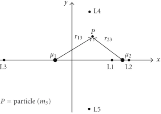
Figure 3.1. Synodic reference system and the relative location of the Lagrangian equilibrium points for Earth-Moon system.
do not have an analytical solution, but they do have symmetry properties that guaran-tee the existence of periodic orbits in the synodic system (Broucke [8]; and Murray and Dermott [16]), such as the Family G orbits that we investigated in this study.
The R3BP also has another interesting property which is the existence of five equi-librium points called Lagrangian equiequi-librium points, symbolized by the letter L. When a particle is placed on these points with a null velocity relative to the origin of the syn-odic system, it remains there indefinitely.Figure 3.1illustrates this synodic system and the relative location of the five Lagrangian equilibrium points for Earth-Moon system.
3.2. Four-body problem. In our numerical simulations, we also considered as dynamical system the four-body problem in three-dimensional space. Thus, for a system of fixed Cartesian coordinates, in which the position of a certain body is given by the vectorxki= (xk1,xk2,xk3)∈R3, the equations of motion are given by
¨ xki=
4
j=1
j=k µj r3
jk
xji−xki, (3.3)
wherek=1, 2, 3, 4;
rjk=xj−xk =
3
i=1
xji−xki2
1/2
(3.4)
based on the Earth’s and Moon’s mass, so thatµ2+µ3=1, then we will haveµ1=µSun=
328 904.4747, µ2=µEarth=0.987 849 396, andµ3=µMoon=0.012 150 604. Considering
that a lunar probe’s mass can vary between some hundreds of kilograms and some tons, its mass parameter,µ4, will be at order of 10−23or 10−24, and even with (3.3) taking into
account the mutual interactions between the four bodies considered, the probe would not influence the motion of the other three. For this reason, the terms of (3.3), which containµ4, were suppressed. This is the four-body Sun-Earth-Moon-probe problem, and
the word restricted could precede it, without a loss of generality, given the order of the size ofµ4. The aforementioned normalization is completed adopting the average distance
between the Earth and the Moon, 384 400 km, as a unit of measurement.
The eccentricity of the Earth’s orbit,e2, the eccentricity,e3, and the inclination,i3, of
the Moon’s orbit were included in the system via initial conditions, thus bringing the system closer to reality. The values for these elements aree2=0.0167,e3=0.0549, and
i3=5.1454◦(relative to the ecliptic).
4. Properties of the Family G orbits
Considering the R3BP, the Family G generally has short-range orbits around L1, long-range orbits that pass a few kilometers from the Earth’s surface and a few dozen kilometers from the Moon’s surface, and even orbits that present a loop. In the synodic system, the first two kinds of orbits have initial conditions of the following type:
x0, 0, 0, ˙y0, (4.1)
while the third kind has initial conditions of the following type:
x0, 0, 0,−y˙0. (4.2)
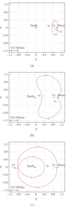
Figure 4.1exhibits an example of each kind, seen in the synodic system. We can ob-serve that for the first two kinds of orbits, pointx0is between the Earth and L1; and point
x1, which corresponds to the first passage by the particle along thex-axis of the
coordi-nate system under consideration, is located between L1 and the Moon. For the third kind, x0is also between the Earth and L1, andx1is located to the left of the Earth, between the
letter and L3. All three kinds of orbits are unstable.
The kinds of paths illustrated inFigure 4.1(b)are those paths capable of making a di-rect transfer between the Earth and the Moon.Figure 4.2exhibits, for the restricted three-body problem, a path of this type, a quasiperiodic orbit. InFigure 4.2(a), it is seen in the synodic system, inFigure 4.2(b), in the geocentric system, together with the Moon’s or-bit, and inFigure 4.2(c), we have a zoom showing a loop given by the path of the Moon’s orbit.
Figure 4.3shows for the four-body problem the orbit obtained with the same initial conditions as inFigure 4.2. Note that with the final approach to the Moon, the probe leaves the Moon’s orbital plane. This fact allows the probe to be inserted into a highly inclined lunar orbit.
−1.2 −0.8 −0.4 0 0.4 0.8 1.2
X
−1.2
−0.8
−0.4 0 0.4 0.8 1.2
Y Earth
153 760 km
x0 L1 Moon x1
(a)
−1.2 −0.8 −0.4 0 0.4 0.8 1.2
X
−1.2
−0.8
−0.4 0 0.4 0.8 1.2
Y Earth
153 760 km
x0 L1 Moon x1
(b)
−1.2 −0.8 −0.4 0 0.4 0.8 1.2
X
−1.2
−0.8
−0.4 0 0.4 0.8 1.2
Y Earth
153 760 km
x0 L1 Moon x1
L3
(c)
−1.5 −1 −0.5 0 0.5 1 1.5
X
−1.5
−1
−0.5 0 0.5 1 1.5
Y
Earth
Moon
384 400 km Family G orbit
(a)
−1.5 −1 −0.5 0 0.5 1 1.5
X
−1.5
−1
−0.5 0 0.5 1 1.5
Y
Earth
384 400 km Moon’s orbit
Initial position Family G orbit
Encounter with Moon int=15.25 days
(b)
−0.98−0.97−0.96−0.95−0.94−0.93−0.92−0.91
X
−0.40
−0.39
−0.38
−0.37
−0.36
−0.35
−0.34
−0.33
−0.32
Y
7688 km Moon’s orbit
Family G orbit
(c)
−1.5 −1
−0.5 0 0.5
1 1.5
X −1.5
−0.5 0.5
1.5
Y
384 400 km
−1.5
−1
−0.50 0.51 1.5
Z Earth Moon’s orbit
Transfer path
Figure 4.3. Path of transfer spatial view in the geocentric system obtained considering the four-body problem Sun-Earth-Moon-probe. The initial condition in the geocentric system is (x0; 0; 0; ˙y0)= (42 370 km; 0; 0; 4.169 km/s).
a terrestrial parking orbit, the injection impulse to acquire a transfer path could only be applied when the Earth, probe, and Moon were all lined up, in this order. For example, for a terrestrial parking orbit with an altitude equal to 200 km, there would be a launching window open every 1.47 hours, a time frame that is not restrictive to using these orbits for transfer maneuvers between the Earth and the Moon.
5. Definition of the set of transfer paths
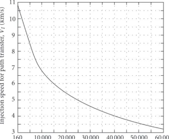
In order to select the paths capable of achieving transfer between a terrestrial and lunar parking orbits, we consider that the probe departs always from a circular orbit around the Earth. We consider altitudes for this orbit,HT, varying between 160 and 20 000 km. Then, we select only those paths that reach the periselenium with altitudes,HL, between 0 and 100 km. This procedure allows us to find a curve that demonstrates the relation between the injection speed for acquisition of a transfer path,VI, and the altitude of the terrestrial circular parking orbit,HT, for transfer path’s periselenium altitude,HL, less than 100 km from Moon’s surface, including collision paths. But if we consider 160≤HT≤700 km, an empirical mathematical expression that relatesVI andHT forHL≤100 km can be written. Considering the four-body problem Sun-Earth-Moon-probe, the mathematical expression is given by
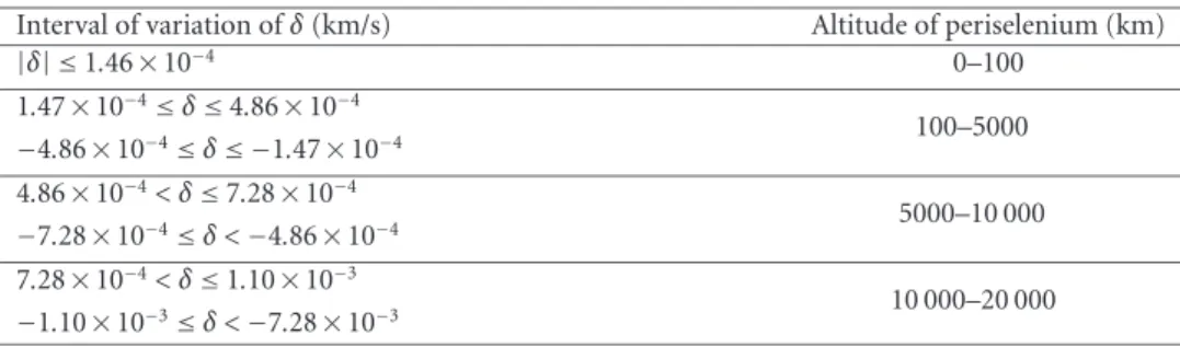
VI= −8.5×10⁻⁴HT+ 11.101 00 +δ. (5.1) The interval 160 ≤HT ≤700 km was chosen taking into account the capacity of present launch vehicles. The set of transfer paths can be seen inFigure 5.1(a), and the set defined by (5.1) inFigure 5.1(b), which is a zoom ofFigure 5.1(a)for 160≤HT≤700 km. Note that for this interval, we have a black band defining the region and not a line, this fact justifies the last term,δ, in (5.1).Figure 5.2shows a zoom of the diagram ofFigure 5.1(b) for 240≤HT ≤245 km. In this figure it is possible to verify the extreme sensitivity of periselenium altitude with injection speed in achieving the transfer path. This structure exists in all the intervals studied, and can be expressed taking into account small varia-tions inδ. These variations are presented inTable 5.1.
160 10 000 20 000 30 000 40 000 50 000 60 000 Altitude of terrestrial circular parking orbit,HT(km),
for periselenium’s altitude of the path,HL, less than 100 km
3 4 5 6 7 8 9 10 11
In
jection
speed
for
p
ath
tr
ansfer
,
VI
(km/s)
(a)
200 300 400 500 600 700
Altitude of terrestrial circular parking orbit,HT(km),
for periselenium’s altitude of the path,HLless than 100 km
10.5 10.6 10.7 10.8 10.9 11
In
jection
speed
for
p
ath
tr
ansfer
,
VI
(km/s)
(b)
Figure 5.1. Injection speed,VI, versus the altitude of the Earth’s parking orbit,HT, for paths with
periselenium,HL, less than 100 km. (a) 160≤HT≤20 000 km and (b) 160≤HT≤700 km.
240 241 242 243 244 245 Altitude of terrestrial circular parking orbit,HT(km),
for periselenium’s altitude of the path,HL, less than 100 km
10.897 10.898 10.899 10.900 10.901 10.902 10.903 10.904
In
jection
speed
for
p
ath
tr
ansfer
,
VI
(km/s)
0–100 km 100–5000 km
5000–10 000 km 10 000–20 000 km
Figure 5.2. Injection speed,VI, versus the altitude of the Earth’s parking orbit,HT, for paths with
various altitudes of periselenium,HL, indicated using a color code.
Table 5.1. Relations betweenδand periselenium altitude.
Interval of variation ofδ(km/s) Altitude of periselenium (km)
|δ| ≤1.46×10⁻⁴ 0–100
1.47×10⁻⁴≤δ≤4.86×10⁻⁴
100–5000
−4.86×10⁻⁴≤δ≤ −1.47×10⁻⁴ 4.86×10⁻⁴< δ≤7.28×10⁻⁴
5000–10 000
−7.28×10⁻⁴≤δ <−4.86×10⁻⁴ 7.28×10⁻⁴< δ≤1.10×10⁻³
10 000–20 000
−1.10×10⁻³≤δ <−7.28×10⁻³
−1.5 −1 −0.5 0 0.5 1 1.5
X
−1.5
−1
−0.5 0 0.5 1 1.5
Y Earth Moon
L1
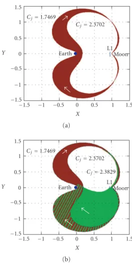
Cj=2.3702
Cj=1.7469
(a)
−1.5 −1 −0.5 0 0.5 1 1.5
X
−1.5
−1
−0.5 0 0.5 1 1.5
Y Earth Moon
L1
Cj=2.3702
Cj=1.7469
Cj=2.3829
(b)
Figure 5.3. “Linking areas” between the Earth and the Moon in the synodic system for the PR3C with (a) 160≤HT≤20 000 km andHL≤100 km and (b) 160≤HT≤20 000 km and 100< HL≤
20 000 km.
leave terrestrial parking orbits with 160≤HT≤5000 km, and decreases gently until 108 degrees for paths with 5000≤HT≤20 000 km.
It is interesting to observe that, in spite of the instability of the paths observed for the two dynamical systems under consideration, they define what we can call “links” between the Earth and the Moon. In order to better understand this, we will consider two paths obtained for PR3C: the first havingHT=160 km,VI=10.969 km/s, that is, in the geocentric coordinates system, (x0; 0; 0; ˙y0)=(6610 km; 0; 0; 10.969 km/s), the
alti-tude of the periseleniumHL=10 km andCJ (Jacob’s constant)=1.7469; and the sec-ond havingHT=20 000 km,VI=3.261 km/s, (x0; 0; 0; ˙y0)=(20 000 km; 0; 0; 3.261 km/s),
−1.5 −1
−0.5 0 0.5
1 1.5
X −1.5
−0.5 0.5
1.5
Y
−1.5
−1
−0.50 0.51 1.5
Z Earth Moon
(a)
−1.5 −1
−0.5 0 0.5
1 1.5
X −1.5
−0.5 0.5
1.5
Y
−1.5
−1
−0.50 0.51 1.5
Z Earth Moon
(b)
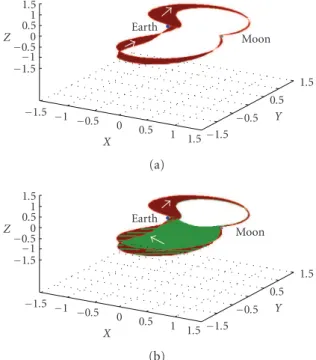
Figure 5.4. “Linking areas and canals” between the Earth and the Moon in the synodic system, ob-tained for the four-body problem with (a) 160≤HT≤20 000 km andHL≤100 km and (b) 160
≤HT≤60 000 km and 100< HL≤20 000 km.
If we also consider that those paths which possess 100 km< HL≤20 000 km as the in-ternal limit of the return “linking area” can be amplified, as shown inFigure 5.3(b), this guarantees faster Moon-Earth transfers.
By analogy, considering paths obtained for the four-body problem with the same init-ial conditions, that are,HT =160 km, VI=10.967 km/s,HL=10 km, i(inclination of the osculating lunar orbit that contains the periselenium)=41.44 degrees, andΩ (lon-gitude of the ascending node of the osculating lunar orbit)=116.87 degrees, andHT= 20 000 km,VI=3.259 km/s,HL=98 km,i=41.89 degrees, andΩ=116.96 degrees, the “area” of the departure journey continues to exist in the Moon’s orbital plane. Nonethe-less, the exit of the transfer path from the Moon’s orbital plane in its final approximation introduces a “break in symmetry,” with relation to that observed for the PR3C. The “area” of the return journey is transformed into a three-dimensional “canal” outside the Moon’s orbital plane and its external limit is different from the external area of the departure journey, as shown in Figures5.4(a)and5.4(b).
6. Flexibility of missions
varying between 160 and 20 000 km, and a lunar parking orbit, with altitude varying be-tween 20 and 20 000 km, and inclination varying bebe-tween 29 and 40 degrees, with appli-cation of only two impulses. The second type of mission utilizes the instability inherent to the paths and gain in inclination to insert them into lunar parking orbits with other inclinations, including polar orbits, at a low cost, applying a∆Vdirectorat mid-journey to
direct the path in such a way that the lunar osculating orbit which contains the perisele-nium has inclinations greater than 40 degrees, or lower than 29 degrees, depending on the mission, of course. Finally, the third type of mission takes advantage of the instability of the paths and the “break in symmetry” caused by their exit from the Moon’s orbital plane during the final approximation. The idea to be exploited is to launch a probe or satellite, towards the Moon in a path defined by (5.1), from a low-altitude terrestrial orbit (LEO), withHT≤700 km, for example, and to take advantage of the gain in inclination and the return linkage “canal” to place the satellite in high-altitude terrestrial orbits and high inclinations, including polar orbits, possibly reducing the cost of this maneuver. Such a maneuver also requires the application of a∆Vdirectorduring mid-flight to adequately
direct the path.
Following we will discuss an example of the first type of mission, that is, a direct trans-fer between a low-altitude terrestrial parking orbit (LEO) withHT=320 km,VI=10.834 km/s, and a lunar parking orbit withHL=84.7 km,i=41.15 degrees, andΩ=116.84 degrees. The∆V1required for the first impulse, the injection impulse that will place the
probe into the transfer path, is the difference betweenVIand the velocity of the terrestrial parking orbit, if we consider the parking orbit as circular, we have
∆V1=VI−
GMEarth
R1
=3.108 km/s, (6.1)
whereR1is the Earth’s parking orbit radius in the point of tangency with transfer path
R1=RT+HT, withRTbeing the Earth’s average radius (6370 km). The∆V2required for
the second impulse, the insertion impulse into the lunar orbit, will correspond to the difference between the velocity of the probe in the periselenium of the transfer path,VP, and the velocity of the planed lunar orbit at the point of its application. Supposing that the plane around the Moon is circular, we have
∆V2=VP−
GMMoon
RP
=0.920 km/s. (6.2)
The value forVP is found through numerical integration, for this exampleVP=2.560 km/s, RP=RL+HL, withRL being the average radius of the Moon (1738 km). In the periselenium of the transfer path, the probe’s velocity is always perpendicular to the Moon-probe position vector, which facilitates the insertion into a circular lunar orbit. The∆VTotalis
The flight time is 13.92 days. The cost of the maneuver calculated by Hohmann is
∆VTotal=3.910 km/s and by patched conic is∆VTotal=4.118 km/s, and the flight time
is of the order of 5 days for both. As we can see, the∆VTotal via the transfer path as
de-fined by (5.1) is greater than the∆VTotalfor the same maneuver via Hohmann (around
3%) and less than the∆VTotalvia patched conic (around 2.2%). However, as we saw in
Section 2, these methods are based strictly upon the dynamics of the two-body Earth-probe and Moon-Earth-probe. Numerical simulations considering the PR3C or the four-body problem show that the∆VTotalvia Hohmann and patched conic are not sufficient to
con-clude the maneuver, requiring corrective∆V’s to compensate for the disturbance caused by the Sun’s and Moon’s gravitational fields (first part of the maneuver) and of the Sun and the Earth (second part). These corrective∆V’s can increase the cost of the maneuver by 5%. On the other hand, the∆VTotalvia the transfer path defined by (5.1) already takes
these disturbances into account.
7. Conclusions
In this study, we have been able to verify the existence of a well-defined set of paths, de-rived from the direct periodic orbits around the Lagrangian equilibrium point L1 (Family G [8]), and capable of carrying out, among other things, a direct transfer maneuver be-tween low-altitude terrestrial and lunar parking orbits. This set was graphically defined starting with injection velocityVI, or velocity required to acquire the transfer path, versus the altitude of the terrestrial parking orbit,HT, for 160≤HT≤20 000 km and withHL (altitude of the lunar parking orbit)≤100 km (Figures5.1and5.2), and via an empirical
mathematical expression for 160≤HT≤700 km (5.1). The dynamical systems consid-ered were the PR3C and the four-body Sun-Earth-Moon-probe problems, to which the eccentricity of the Earth’s orbit and the eccentricity and inclination of the Moon’s orbit were taken into account.
In addition to the direct transfer between the Earth and the Moon, the paths defined by the graphs in Figures5.1and5.2can also be used to insert a probe into lunar orbits with high inclinations, including polar orbits, thanks to the instability and to the fact that they leave the Moon’s orbital plane in their final approximation. It is also possible to exploit this gain of inclination to transfer, at a low cost, a probe or a satellite from a low-altitude terrestrial orbit (LEO), to an orbit with a much higher low-altitude, with or without high inclinations. This maneuver is possible because the set of investigated paths defines “linking areas” and/or “canals” between the Earth and the Moon, as shown in Figures4.3, 5.3, and5.4.
With respect to the cost of the direct transfer maneuver, when compared to the con-ventional methods of Hohmann and patched conic, we see that the paths studied have
∆VTotalthat are very close to those obtained by these methods. However, the∆V’s found
the conventional methods are unbeatable, but a flight time between 13 and 15 may be acceptable in logistical missions, transfer of automatic probes, and even in some manned missions given the presumed savings.
When compared to the traditional gravitational capture transfer methods, in general, the cost of a maneuver carried out by a path defined in (5.1), for example, is greater (around 5%). However, the flight times for gravitational capture transfers are very long, and are measured in months (7–16), while flight times for the paths herein presented do not exceed two weeks.
Therefore, we can conclude that this study reveals a set of alternative paths for transfer missions in the Earth-Moon system that, if properly exploited, could reduce the costs of some important maneuvers in the present context and also in the future of space explo-ration.
Acknowledgment
The authors are grateful to the FAPESP (Fundac¸˜ao de Amparo `a Pesquisa do Estado de S˜ao Paulo) and the CNPq (Conselho Nacional para Desenvolvimento Cient´ıfico e Tec-nol ´ogico), Brazil.
References
[1] R. R. Bate, D. D. Mueller, and J. E. White,Fundamentals of Astrodynamics, Dover, New York, 1971.
[2] E. A. Belbruno,Lunar capture orbits, a method of constructing earth moon trajectories and the lu-nar gas mission, Proceedings of 19th AIAA/DGLR/JSASS International Electric Propulsion Con-ference, Colorado Springs, Colorado, 1987, AIAA-87-1054.
[3] ,Examples of the nonlinear dynamics of ballistic capture an escape in earth moon system, Proceedings of AIAA Astrodynamics Conference (Oregon, 1990), American Institute of Aero-nautics and AstroAero-nautics, Washington, DC, 1990, pp. 179–184, AIAA-90-2896.
[4] ,Ballistic lunar capture transfer using the fuzzy boundary and solar perturbations: a survey, Proceedings of International Congress of SETI Sail and Astrodynamics (Turin, 1992), 1992. [5] ,Through the fuzzy boundary: a new route the moon, The Planetary Report7(1992),
no. 3, 8–10.
[6] E. A. Belbruno and J. K. Miller,A ballistic lunar capture trajectory for Japanese spacecraft Hiten, International Document JPL IOM 312/90.4-1731, Jet Propulsion Laboratory, California Insti-tute of Technology, California, 1990.
[7] ,Ballistic lunar capture for the lunar observe, Internal Document IOM 212/90.4-1752, Jet propulsion Laboratory, California Institute of Technology, California, 1990.
[8] R. A. Broucke,Periodic orbits in the restricted three-body problem with earth-moon masses, Tech. Rep. 32-1168, Jet Propulsion Laboratory, California Institute of Technology, California, 1968. [9] A. Brunini,On the satellite capture problem, capture and stability regions for planetary satellites,
Celestial Mechanics & Dynamical Astronomy.64(1996), no. 1-2, 79–92.
[10] W. C. Feldman, B. L. Barraclough, S. Maurice, R. C. Elphic, D. J. Lawrence, D. R. Thomsen, and A. B. Binder,Major compositional units of the moon: lunar prospector thermal and fast neutrons, Science281(1998), no. 5382, 1489–1493.
[11] W. S. Koon, M. W. Lo, J. E. Marsden, and S. D. Ross,Low energy transfer to the moon, Celestial Mechanics & Dynamical Astronomy.81(2001), no. 1-2, 63–73.
(South Carolina, 1990), American Institute of Aeronautics and Astronautics, Washington, DC, 1992, pp. 435–444, AIAA-1992-4581.
[13] M. W. Lo and S. D. Ross,Low energy interplanetary transfers using invariant manifolds of L1, L2 and halo orbits, Proceedings of AAS/AIAA Space Flight Mechanics Meeting (California, 1998), 1998.
[14] J. K. Miller and E. A. Belbruno,A method for construction of a lunar transfer trajectories using ballistic capture, Proceedings of 1st AAS/AIAA Annual Spaceflight Mechanics Meeting (Texas, 1991), 1991, pp. 97–109, AAS-91-1000.
[15] M. A. Murison,The fractal dynamics of satellite capture in the circular restricted three-body prob-lem, Astronom. J.98(1989), no. 6, 2346–2359.
[16] C. D. Murray and S. F. Dermott,Solar System Dynamics, Cambridge University Press, Cam-bridge, 1999.
[17] C. A. Ocampo,Transfers to earth centered orbits via lunar gravity assist, Acta Astronaut.52(2003), no. 2, 173–179.
[18] A. F. B. A. Prado,Minimun fuel trajectories for the lunar polar orbiter, Revista Brasileira de Automac¸˜ao e Controle (SBA).12(2001), no. 2, 163–170 (portuguese).
[19] ,A numerical study of the gravitational capture in the bi-circular restricted four-body prob-lem, Proceedings of 54th International Astronautical Congress (Bremen, 2003), 2003, IAC-03-A.1.01.
[20] A. F. B. A. Prado and E. Vieira Neto,Orbital maneuvers using gravitational capture, nonlinear dynamics, chaos, control and their applications to engineering sciences, New Trends in Dynamics and Control (J. M. Baltazar, P. B. Gonc¸alves, and R. M. F. L. R. F. Brazil, eds.), vol. 3, 2002, pp. 109–128.
[21] P. A. Regeon, P. R. Lynn, M. Johnson, and R. J. Chapman,The clementine lunar orbiter, Proceed-ings of 20th GIFU ISTS & 11th IAS, Paper no. 96-e-40, 2002.
[22] O. C. Winter, E. Vieira Neto, and A. F. B. A. Prado,Orbital maneuvers using gravitational capture times, Advances in Space Research31(2003), no. 8, 2005–2010.
[23] H. Yamakawa,On earth-moon transfer trajectory with gravitational capture, Ph.D. dissertation, University of Tokyo, Tokyo, 1992.
Cristiano Fiorilo de Melo: Programa de P ´os-graduac¸˜ao em Engenharia e Tecnologia Espaciais, Instituto Nacional de Pesquisas Espaciais (INPE), 12245-970 S˜ao Jos´e dos Campos, SP, Brazil
E-mail address:[email protected]
Othon Cabo Winter: Grupo de Dinˆamica Orbital & Planetologia, Universidade Estadual Paulista (UNESP), Campus Guaratinguet´a, 12516-410 Guaratinguet´a, SP, Brazil;
Programa de P ´os-graduac¸˜ao em Engenharia e Tecnologia Espaciais, Instituto Nacional de Pesquisas Espaciais (INPE), 12245-970 S˜ao Jos´e dos Campos, SP, Brazil
Impact Factor
1.730
28 Days
Fast Track Peer Review
All Subject Areas of Science
Submit at http://www.tswj.com
Hindawi Publishing Corporationhttp://www.hindawi.com Volume 2013 Hindawi Publishing Corporation