Nonequilibrium Nematic-Isotropic Interface
Oscar Nassif de MesquitaDepartamento de Fisica
ICEX, Universidade Federal de Minas Gerais C.P. 702, Belo Horizonte 30161-960, MG
Received28October,1998
Liquid crystals have been very fruitful systems to study equilibrium phase transitions. Re-cently, they have become an important system to study dynamics of rst-order phase tran-sitions. The moving nonequilibrium nematic-isotropic interface is a model system to study growth of stable states into metastable states and displays a myriad of dynamical insta-bilities that, far from equilibrium, drive the system to a scenario of spatio-temporal chaos. We present a mean-eld theory for the time evolution of a planar nonequilibrium nematic-isotropic interface for pure liquid crystals using a time dependent Ginzburg-Landau equation, which is one of the simplest approaches to dissipative dynamics. We obtain a theoretical expression for the growth kinetics of the nematic phase into a metastable isotropic phase and compare it with our experimental results. In a directional solidication arrangement we study instabilities of the nematic-isotropic interface of the liquid crystal 8CB doped with water and hexachloroethane. The observed instabilities are similar to cellular instabilities that appear during growth of crystal-melt interfaces of binary mixtures. We then compare our results with known theories of morphological instabilities during crystal growth.
I Introduction
Equilibrium thermodynamics has contributed much to the understanding of a variety of physical phenomena. Like other areas of Physics, equilibrium thermodynam-ics is based on some variational principle (maximum entropy or minimum free-energy), such that if we know the free-energy of the system then we are able to predict all the properties of its, in general, unique equilibrium state.
The diversity of shapes, forms (including living forms) in Nature, certainly could not be explained by equilibrium thermodynamics. We do not know if nonequilibrium thermodynamics can explain all that either, but at least it opens up some new possibili-ties. In nonequilibrium thermodynamics, history (time evolution) assumes its importance leading the system to a variety of dierent states, other than equilibrium states, as energy is continuously pumped into it. When the input of energy ceases, the system then evolves to its equilibrium state - that is the boring state of death for living forms. On the other hand, nonequilibrium
systems display a variety of rich and complex dynami-cal phenomena, self-organization and pattern formation giving rise to a great diversity of forms.
As far as I know, there is nothing like a general variational principle for nonequilibrium thermodynam-ics. We cannot say in general that the time evolution or steady-states of nonequilibrium systems are determined by some principle like minimum dissipation of energy, or other like maximum production of entropy. In some especial cases these principles work and in others they do not work, raising some doubts about the usefulness of such general principles. In hydrodynamic systems one can nd both situations [1 ] [2 ] . Therefore, the usual approach to study nonequilibrium systems is to consider each case and look for some universal behavior. Here, universal behavior means that the time evolution and steady-states of several dierent real systems can be grouped and described by solutions of a particular, usually phenomenological, nonlinear partial dierential equation [2 ].
sit-uations, both with very rich dynamical behavior. In one case we shall discuss, for pure liquid crystals, the motion of a planar nematic-isotropic interface when the temperature of the system is quenched below its equilibrium nematic-isotropic transition temperature, such that the nematic phase (stable phase) grows into the isotropic phase (metastable phase). Which order-parameter-shape-prole and front velocity will be se-lected out from several possible solutions of nonlinear equations is what we would like to determine. One of the simplest equations for dissipative dynamics is a time-dependent Ginzburg-Landau equation [3 ] [4 ] [5 ]. We will derive the kinetics of the nematic-isotropic interface based on this equation, discuss the velocity-selection problem and then compare the results with our kinetic measurements [6 ] [7 ].
In the second situation, we will describe morpho-logical instabilities that occur in the moving nematic-isotropic interface of doped systems using an experi-mental conguration of directional solidication. These instabilities (cellular and dendritic) have been studied for more than 30 years [8 ] [9 ] [10 ] in the context of crystal-growth, because they are very important for material processing. They are the main responsible for the microstructure of cast metals, and, consequently, responsible for their mechanical and electrical proper-ties. More recently, the cellular instability was shown to occur also in liquid crystals [11 ] [12 ] [13 ], dis-playing a variety of new dynamical phenomena and a scenario of spatio-temporal chaos [14 ] [15 ]. Since for liquid crystals the parameters for triggering the cellular instability and time scales involved are more amenable to laboratory conditions, the moving nematic-isotropic interface has become a model system to study com-plex dynamics and pattern formation. We will discuss the physical origin for the onset of the cellular insta-bility and show some of our more recent data for the moving nematic-isotropic interface of the liquid crystal 8CB doped with hexachloroethane and water.
II Nematic-isotropic phase
tran-sition
A. Pure systems
The nematic-isotropic phase transition in liquid
crystals is a weakly rst-order transition. In the ne-matic phase the rodlike anisotropic molecules inter-act to create a long-range orientational order. The molecules are aligned, in the average, along a partic-ular direction dened by a vector ,!
n, the director. In
the nematic phase the center of mass of the molecules are not correlated, therefore, concerning the translation degrees of freedom the liquid crystal behaves as a liq-uid : an anisotropic liqliq-uid. The quadrupolar ordering of the nematic phase can be described by a traceless tensor, the order parameter tensor, given by [16 ]
Q
=
Q
2 (3n
n
,
) (1)
where n
are the components of the director vector , !
n
andQ(0Q1) is the modulus of the order
param-eter. As seen in other articles of this issue, the Landau-de Gennes theory [16 ] can proviLandau-de a phenomenologi-cal mean-eld description of phase transitions in liquid crystals. The Landau-de Gennes free energy density for nematic liquid crystals can be written as,
F =F 0+ 12
C 1
Q
Q + 13
C 2
Q
Q
Q
+
::::
(2) whereF
0is the free energy density of the isotropic phase
andC 1
;C 2
;etc., are constants.
In our experiments, the liquid crystal 8CB is sand-wiched between glass slides. Typical sample thicknesses vary from 3 to 5 m. The internal surfaces of the
cover glasses which are in contact with the liquid crystal are treated with silane, what guarantees a homeotropic conguration for the nematic phase, i.e., the director,! n
is perpendicular to the cover glass surfaces. In this sim-plied geometry, whereQ
zz = Q,Q
yy= Q
xx= ,Q=2 Q
xy= Q
yz= Q
xz= 0 , the Landau-de Gennes free
en-ergy density can be written in terms of the scalar order parameterQas,
F = 12AQ 2
,
1 3BQ
3
+ 14CQ 4
+ 12a 2 0 T
@Q @z
2
(3) whereA;B;Cand
0are phenomenological coecients
whose values must be determined empirically from ex-periments. As usual, one assumes that the main tem-perature dependence is contained in Asuch that A = a(T,T
) , where
T is temperature,T
is the
occur if B=0 exactly, and a is a constant. The
coe-cient of the gradient term is also a constant which we wrote as a
2 0 T
, anticipating future results.
0 is the
bare correlation length with dimension of the order of the molecular size. Without losing generality we set the free energy F
0 of the isotropic phase equal to zero. A
schematic view of this free energy as a function of the order parameter for dierent temperatures and with-out the gradient term, can be seen in Fig.1. TNI is
the nematic-isotropic transition temperature and QNI
is the order parameter at the transition. The free en-ergy without the gradient term can describe homoge-neous phases. In order to describe the nematic-isotropic interface we have to include it. Let us use the homo-geneous free energy (no gradient term) to make some predictions for the homogeneous phases.
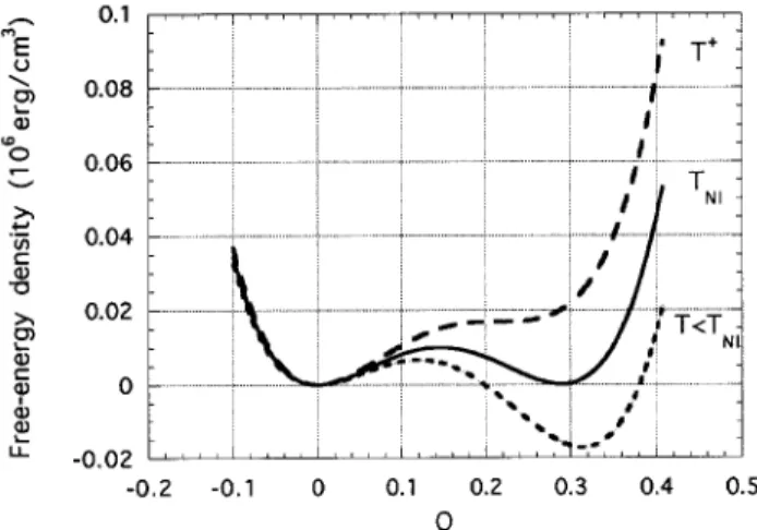
Figure 1. Plot of Landau-de Gennes homogeneous free en-ergy densityF for the nematic-isotropic phase transition as a function of the scalar order parameterQ, for dierent tem-peratures. Parameters used are for the nematic-isotropic transition of the liquid crystal 8CB.
To nd the conditions describing a rst-order phase transition we shall, as usual, minimize the free en-ergy density and impose the coexistence between the isotropic and nematic phases, i.e., @F=@Q = 0 and F(Q
NI) =
F(0) = 0 , where Q
NI is the value of the
order parameter of the nematic phase at the transition temperature T
NI and
Q= 0 is the value of the order
parameter of the isotropic phase. Note that the temper-ature T
NI is dierent from the phantom second-order
transition temperatureT
. By imposing the conditions
above we nd:
T NI
,T
= 29B 2
aC
; (4)
Q NI = 23
B C
: (5)
From Fig.1 we see that for T > T
NI, the nematic
phase (Q6= 0) has a local minimum (metastable phase)
while the isotropic phase (Q= 0) has an absolute
mini-mum (stable phase). ForT <T
NI the opposite occurs:
the nematic phase is the stable one while the isotropic is the metastable phase. AtT =T
, @
2 F=@Q
2= 0 ,
forQ = 0 , therefore the isotropic phase becomes
ab-solutely unstable. We also dene the temperatureT + ,
given byT + ,T NI = 1 8( T NI ,T ), where @ 2 F=@Q
2= 0,
forQ +=
3 4
Q
NI, such that the nematic phase becomes
absolutely unstable. Therefore, the metastable region occurs forT
T T
+ and this is the temperature
interval where a nematic-isotropic interface can exist. A fundamental question that must be answered is how fast one phase grows at the expenses of the other, when the system is quenched from one temperature to an-other. This question is not trivial to answer and great eorts have been put into it in the last decades [3 ] [4 ] [5 ] . This is the sort of question that we would like to answer when we consider a nonequilibrium nematic-isotropic interface.
1. Nematic-isotropic interface
AtT
NI the nematic and isotropic phases can
coex-ist, separated by a stationary interface. If we consider the complete free energy density given by Eq. (3) and imposing the boundary conditionsQ(z= +1) = 0 and Q(z =,1) =Q
NI , we can nd the prole for Q(z).
To minimize the free energy density (F=Q = 0) we
then solve the Euler-Lagrange equation associated with Eq. (3). The resulting equation is
a 2 0 T @ 2 Q @z 2 =
AQ,BQ 2+
CQ
3 (6)
with solution
Q(z) = Q
NI
2
1,tanh
z
2
(7) where the correlation length is related to the bare
correlation length 0 by = 0 r T
T ,T
The interface is located atz= 0 and its width is
de-termined by . The equilibrium nematic-isotropic
sur-face tension can be calculated using the excess sursur-face free energy denition [17 ] [5 ]
e= Z +1 ,1 1 2A e 2 e @Q @z 2
dz= 16A e e Q 2 NI (9)
where all the quantities are calculated at T NI.
2. Nonequilibrium nematic-isotropic interface
If we prepare the system initially at the equilibrium temperature T
NI , with boundary conditions
Q(z =
+1) = 0 andQ(z = ,1) = Q
NI , we will have the
proleQ(z) given by Eq. (7). Then we quench the
tem-perature to a value smaller than T
NI but larger than T
. The interface will start to move towards positive z,
i.e., the nematic phase starts to grow at the expenses of the isotropic phase. It has been proposed in the lit-erature some theoretical frameworks to compute this velocity as a function of temperature. We will describe below the simplest one for dissipative dynamics based on a time dependent Ginzburg-Landau equation, given by [3 ] [4 ] [5 ] [18 ]
@Q @t =, F Q (10) where is a viscosity associated with the ordering of
the nematic phase. A transport parameter that can be measured directly is the rotational viscosity of the ne-matic liquid crystal
1, which is related to
by [5 ]
[18 ] = 1 3Q 2 NI : (11)
The equation we have to solve is then,
@Q @t =a 2 0 T @ 2 Q @z 2
,AQ+BQ 2
,CQ 3
: (12)
We look for stationary solutions moving with con-stant speed like Q(z , Vt). By changing variable, s=z,Vt, we obtain,
a 2 0 T d 2 Q ds 2 + V dQ ds
,AQ+BQ 2
,CQ 3= 0
:
(13) We can try a solution of the type,
Q(s) =
2
h
1,tanh
s
2
i
(14)
where and are to be determined. We will show
that this is indeed a solution of Eq. (13). This is not, however, the only solution. The velocityV depends on
the shape of the interface. We can nd a great num-ber of shape solutions each one moving with dierent speed. Ben Jacob et al. and later W. van Saarlos [19 ] [4 ] , made a nonlinear marginal stability analysis of propagation of fronts into metastable states described by an equation of the type of Eq. (13). They showed that, within the metastable range, the only selected ve-locity is the one of a moving front with prole dened by Eq. (14). Then we can use this prole and uniquely determine the velocity of the front.
We substitute Eq. (14) into Eq. (13) and obtain,
= 34Q NI " 1 + s 1, 8 9 (
T,T ) (T NI ,T ) # = 43 e h
1 +q
1, 8 9 (T,T ) (TNI,T ) i
and nally, the expression for the front velocity is
V = 34 a e (T NI ,T ) "s
1,8
T,T NI T NI ,T ,1 # : (15) IfT <T
NI the interface moves towards positive z
and it is supercooled. If T >T
NI the interface moves
towards negative z and it is superheated. The dierence T =T ,T
NI is called supercooling or superheating
depending on its sign. From Eq. (15), for tempera-tures aboveT
+, the front velocity becomes imaginary:
the nematic phase is absolutely unstable. For the liq-uid crystal 8CB, T
NI ,T
is equal to 2K, therefore T
+ ,T
NI is equal to 0.25K. In fact we observe, even
for small superheatings like 0.3K , that the interface disappears and the transition resembles a second order transition.
For a rst order transition and very small supercool-ings or superheatsupercool-ings the velocity of the front should vary linearly with T . If we expand Eq. (15)
impos-ing that T =T,T NI
<<(T NI
,T )
=8 we obtain,
V = 3 a
e
(T NI
,T) : (16)
than 0.25K. This short temperature interval for the linear behavior is a characteristic of weakly rst-order transitions. For instance, in the case of crystal-melt in-terfaces this linear behavior can extend to larger tem-perature intervals. We will t our data of velocity as a function of temperature using the complete Eq. (15).
In the above analysis we have neglected the latent heat liberated during the motion of the interface. In the case of the nematic-isotropic transition of the liq-uid crystal 8CB the latent heat generated is very small and can be safely neglected. This is one of the advan-tages of studying kinetics of nematic-isotropic interfaces rather than crystal-melt interfaces. In addition, for the nematic-isotropic interface the Landau-de Gennes free energy formulation can give reasonable results and then we can make predictions based on this free energy, like the velocity of the front shown above. For regular crystal-uid interfaces, as far as I know, there is no such free energy description for the problem.
B. Doped systems
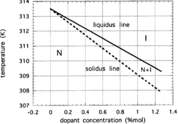
If we introduce dopants that are soluble or par-tially soluble into the liquid crystal, a binary phase will emerge. For very low concentrations a sketch of a bi-nary phase diagram is shown in Fig. 2. There we show a situation where the dopant decreases the free energy of the solvent, then the transition temperature decreases as the concentration of dopant increases. Also, a region of coexistence of nematic and isotropic phases appears between the liquidus and solidus lines. The liquidus and solidus temperatures can be written as
TL=TNI ,m
LCI (17:a)
TS=TNI ,m
SCN ; (17:b)
where mL and mS are the liquidus and solidus slopes
and CN and CI are the dopant concentrations in the
nematic and isotropic phases respectively. For a given temperature the dopant concentration in the nematic phase (CN) is in equilibrium with a dopant
concentra-tion in the isotropic phase (CI) , such that the ratio
CN=CI = mL=mS = K, where K is the segregation
coecient. In the present caseK <1 .
Figure 2. Partial plot of a phase diagram for a binary mixture with segregation coecient K smaller than one. The transition temperature decreases linearly with increas-ing dopant concentration, for small dopants concentrations. Below the solidus line is the nematic phase (N), above the liquidus line is the isotropic phase (I), between the two is a region of coexistence of the two phases (N+I). Parameters used are for water in 8CB withK = 0:75 andmL = 3:33 K/%mol.
Figure 3. Directional solidication apparatus. A thin sample of liquid crystal sandwiched between glass slides is placed in contact with two aluminum blocks, one above and the other below the nematic-isotropic transition tempera-ture, separated by a 1 cm glass gap. The nematic-isotropic interface is visualized in the gap with a microscope con-nected to a video-system. As the sample is pulled towards the colder block the nematic phase starts to grow. We can revert the pulling system and also melt the nematic phase. The motion of the interface is then video-recorded for pos-terior analysis.
Let us consider now a experimental situation where the liquid crystal is sandwiched between glass slides as mentioned before and put in a directional solidication oven like in Fig. 3. The oven consists of two metal blocks separated by some distance. One of the metal blocks has temperature aboveTNI and the other below,
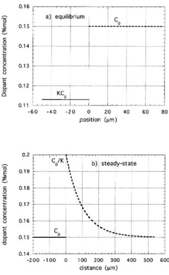
the two blocks. A nematic-isotropic interface will ap-pear in the space between the two blocks. This interface can be visualized by an optical microscope coupled to a video system. A schematic plot of the equilibrium con-centration of dopants is shown in Figure 4a. By using a pulling system we start to pull the sample towards the colder block, then the nematic phase starts to grow. We follow the motion of the interface until it becomes stationary in the laboratory frame. At this situation we know that the interface is moving with the same ve-locity as the pulling veve-locity. SinceK<1 ,C
N <C
I,
then as the nematic phase grows it segregates dopants at the interface, then the dopant concentration at the isotropic side of the interface starts to build up. The steady-state situation is achieved when the segregated dopant ux equals the dopant ux due to diusion in both phases. The transport equations for the dopants in the system of reference of the moving interface are given by [9 ] [10 ],
@C N @t
=D N
@ 2
C N @z
2 + V
@C N @z
(z<0) (18:a)
@C I @t
=D I
@ 2
C I @z
2 + V
@C I @z
(z>0) (18:b)
with boundary conditions,
VC I(1
,K) =D N
@C N @z
,D I
@C I @z
at the interface
(z= 0); (18:c)
C N(
z=,1) =C I(
z= +1) =C 0
; (18:d)
where D N ,
D
I , are the diusion coecients of the
dopant in the nematic and isotropic phases respectively, V is the velocity of the interface and C
0 is the
ini-tial dopant concentration in the isotropic phase. The steady-state solution for this problem is given by,
C N(
z) =C 0 for
z<0; (19:a)
C I(
z) =C 0
1 + 1,K K
exp
,
V D I
z
forz>0:
(19:b)
A steady-state dopant concentration prole given by Eq (19:b) is shown in Fig. 4b. The liquidus
tempera-ture ahead of the interface and the actual temperatempera-ture
prole in the sample is shown in Fig. 5. If the external temperature gradient is such that the actual tempera-ture of the interface is smaller than the liquidus tem-perature (like in the case of Fig. 5), the liquid ahead of the interface is supercooled (\constitutional supercool-ing"). The interface is then growing into a metastable phase, then instabilities occur: the planar interface be-comes cellular. This morphological instability is named Mullins-Sekerka instability [8 ] and has been the sub-ject of intense research for the last 30 years [8 ] [9 ] [11 ] [15 ] [12 ] [13 ] .
Figure 4. a) Equilibrium dopant concentration at the nematic-isotropic interface (V = 0). Parameters are for water in 8CB: K = 0:75 and dopant concentration in the isotropic phase equal toC0= 0:15% (saturation concentra-tion of water in the isotropic phase). Interface is atz= 0, nematic phase is atz <0 and isotropic phase is atz >0; b) Steady-state dopant concentration prole at a moving nematic-isotropic interface with velocity V = 0:7m=s, as predicted by Eq. (19.a) and Eq. (19.b). Interface is at
z = 0, nematic phase is at z < 0 and isotropic phase is at z > 0. Parameters used are for water in 8CB with
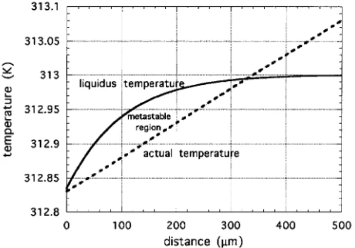
Figure 5. Continuous line is the liquidus temperature in the isotropic side of the interface for the steady-state dopant concentration prole of Fig. 4b, given by Eq. (17.a), with
TNI = 313:5 K andmL= 3:33 K/%mol. The dashed line represents the external temperature prole determined by the temperatures of the ovens of the directional solidication apparatus. In the case shown here the temperature gradi-ent G= 5 K/cm such that, near the interface, the actual temperature of the isotropic phase is below the transition (liquidus) temperature (constitutional supercooling). The interface is then moving towards a metastable phase, then cellular instabilities can occur. By increasing the external temperature gradient, or decreasing the growth velocity this instability can be avoided.
We are interested on the weakly non-linear regime of such instabilities, where a simple phenomenological description is possible. If only few Fourier modes of the interface deformations are unstable and the rest is damped due to dissipation, we can describe the dynam-ics by a simple Landau amplitude equation of the type [2 ] [10 ],
@A @t
=!A,jAj 2
A (20:a)
where A is the amplitude of the most unstable spatial
Fourier mode,!is the growth rate of this mode andis
the third-order coecient. This is the simplest Landau equation allowed by the symmetry of the problem.
A solution to Eq. (20.a) is,
jAj= 2
4 v u u t
!
+ 1
jA 0
j 2
, !
!
exp(,2!t) !
3
5 ,1
:
(20:b)
whereA
0is the initial amplitude at
t= 0. The behavior
above has been observed in hydrodynamic systems spe-cially for the Rayleigh-Benard instability [2 ]. The rst demonstration of this universal behavior in directional
solidication was made by us [12 ], using a nonequilib-rium nematic-isotropic interface. As the growth veloc-ity is increased the system is taken far from equilibrium, secondary instabilities starts to occur and the interface can become chaotic. Coullet et al. [20 ] showed that the symmetry of the problem allows 10 dierent secondary instabilities. Some of them have been already observed [15 ] . Kassner et al. [14 ] have studied some of the scenarios of spatio-temporal chaos in this system.
We shall later present our data displaying some of these instabilities. The nonequilibrium nematic-isotropic interface is a very rich system to study nonequilibrium dynamics and pattern formation.
III Experiments
A. Kinetic measurements for pure systems
Kinetic measurements are done with pure liquid crystal 8CB. The system initially in the isotropic phase at temperatures little aboveT
NI is quenched down to
temperatures slightly below T
NI. A moving
nematic-isotropic interface is then observed and recorded with video techniques. Velocity of the front is measured as a function of temperature. The apparatus oven is made with a large copper block and visualization of the inter-face is made with an optical microscope through sap-phire windows. Sapsap-phire windows are used because of their high heat conduction coecient, such that the temperature prole in the sample is little aected by the ambient temperature and stays very uniform and stable. The temperature is monitored by a thermocou-ple inside of the copper block. Temperature stability is of 0:01K during the time interval of each run. The
relaxation time for thermal equilibrium after quenching the temperature is around 3s. We position the micro-scope at the opposite end of our 7 cm sample in relation to where the interface starts, such that the actual data is taken after the temperature has equilibrated. Clearly, we cannot safely measure very fast interfaces with high supercoolings, then we limit the measurements to in-terface velocities up to 5 to 6 mm/s, which will take about 10s to enter the eld of view of the microscope, i.e., minimum of 3 times the thermal relaxation time.
an expression like Eq. (15), where we use the value
TNI ,T
= 2K for 8CB, such that
V = p
1,4(T,T NI)
,1
;
and with the help of Eq. (11) we get,
= 34ae
= 92aeQ 2 NI
1
:
Figure 6. Plot of the velocity V of the moving planar nematic-isotropic interface as a function of temperatureT. The circles with error bars are the experimental data for the pure liquid crystal 8CB. Continuous line is a t to Eq. (15).
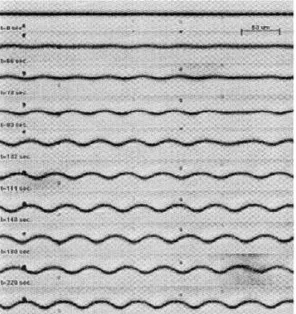
Figure 7. Time series of a doped moving nematic-isotropic interface undergoing a cellular instability.
From the tting we obtain the value =3:10:5
mm/sK . We have to compare this value with the the-oretical prediction above. The measurements of the ro-tational viscosity1were made by Viana et al.[6 ] [7 ] ,
using the technique of optical birefringence. NearTNI
its value is1 = 0:25
0:05 poise. The values for the
other parameters were measured by Faetti et al. [17 ] and are,
a= (1:90:1):10
6erg=cm3K
e= (18 +17 ,10):10
,8cm
QNI = (0:29
0:01) .
With these values we obtain
= 5:2 mm/sK , with a lower limit of 2:3 mm/sK and upper limit of 10:4 mm/sK . The largest error comes from the measurements of the correlation length. Our result falls within this range.
B. Morphological instabilities in doped systems
Our measurements of instabilities on the moving nematic-isotropic interface is done in a directional so-lidication apparatus described earlier and presented in Fig. 3. The sample consists of the liquid crystal 8CB doped with 1%mol of hexachloroethaneC2Cl6, or with
0.15 %mol of water. In this paper we just want to give a avor about the possibilities and wealth of dynamical phenomena that the nonequilibrium nematic-isotropic interface displays. For a more complete description of experiments made by us and novel results with applied electric eld see references [12 ] [13 ] and [21 ] .
Figure 8. Circles are the measured amplitude of the most unstable spatial Fourier mode of the interface of Fig. 7, as a function of time. Continuous line is a t using a solution of the third-order Landau amplitude equation given by Eq. (20:b).
(20.a). From the tting we obtain the growth rate of the most unstable mode!and the third-order
coe-cient. In a previous article we showed that in the regime where a third-order Landau equation ts well the data, the results are consistent with the theory of Caroli et al. [10 ] for this instability. As we increase growth ve-locity, secondary instabilities start to appear and the dynamical behavior of the interface becomes very com-plex. An example of a secondary instability is shown in Fig. 9. This is an vacillating-breathing instability, where the interface shows a spatial period-doubling os-cillatory instability. The cell width oscillates in phase opposition with its neighbors (vacillation) and we also notice that the cell top oscillates in a breathing fashion. These motions are quasi-periodic and eventually the in-terface becomes chaotic [14 ] . In Fig. 10 we show the time evolution of the main spatial Fourier mode of the patterns shown in Fig. 9. The oscillations are quasi-periodic and the system evolves to a scenario of spatio-temporal chaos.
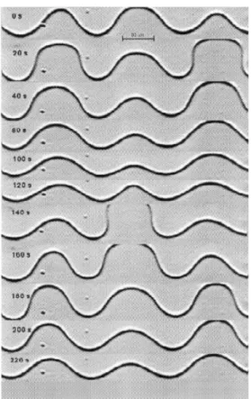
Figure 9. Time sequence of a moving nematic-isotropic in-terface undergoing a vacillating-breathing instability. Note that the cell width oscillates in phase opposition with its neighbors (vacillation) while the cell top oscillates in a breathing fashion. t=0 s in this gure corresponds to t=1500 s in the actual experiment.
Figure 10. Amplitude of the most unstable spatial Fourier mode of the nematic-isotropic interface from Fig. 9, as a function of time. Pictures shown in Fig. 9 correspond to interface shapes recorded from t=1500 s, while the plot of the Fourier amplitude is for the whole run. We see a quasi-periodic motion due to the vacillating-breathing instability. Later on, the interface became chaotic.
More complex dynamical situations can be obtained and a more complete characterization of these sec-ondary instabilities are under way in our laboratory.
IV Conclusions
comparison with theoretical models. We present some examples of the nematic-isotropic interfaces undergo-ing a cellular instability. Also we showed an example of a vacillating-breathing secondary instability which can drive the system to a scenario of spatio-temporal chaos. As the system becomes far from equilibrium , very com-plex dynamical behavior occurs. Liquid crystals oer new possibilities as compared to regular solid-uid sys-tems, because the degree of order in both phases can be varied under the action of electric elds. Since the applied electric eld can be varied continuously, some parameters like segregation coecient, capillary length and anisotropy of the surface tension may as well be varied continuously. Since this feature is unique for liq-uid crystals, this opens up new interesting possibilities for experiments. Interesting experiments would be on the cellular-dendritic transition and test of the theory of microscopic solvability for dendrites, both requiring a continuous variation of surface tension anisotropy.
In this paper we reviewed two dierent aspects of the moving nematic-isotropic interface problem. Hope-fully, it will give to the readers a avor about this area of research and about the wealth of phenomena and com-plex dynamical behavior that this conceptually simple system can display.
V Acknowledgments
I would like to thank the members of our Statisti-cal Physics Group specially Prof. J.M.A. Figueiredo, Prof. J.K.L. Silva and the students Orlando A. Gomes, Nathan B. Viana and Ubirajara A. Batista. Work in our laboratory has been sponsored by FAPEMIG and fellowships provided by CNPq .
References
[1 ] Paul Manneville, Dissipative Structures and Weak Turbulence, Academic Press, New York, 1990. [2 ] M.C. Cross and P.C. Hohenberg, Rev. Mod. Phys.65,
851 (1993).
[3 ] Wim van Saarlos, Phys. Rev. A37, 211 (1988). [4 ] Wim van Saarlos, Phys. Rev. A39, 6367 (1989). [5 ] V. Popa-Nita and T.J. Sluckin, J.Phys. II France 6,
873 (1996).
[6 ] Nathan B. Viana, Master's Thesis, UFMG, Belo Hor-izonte, Brasil (1998).
[7 ] Nathan B. Viana, J.K.L. Silva, O.N. Mesquita and J.M.A. Figueiredo, submitted to publication (1998). [8 ] W.W. Mullins and R.F. Sekerka, J. Appl. Phys. 34,
323 (1963) ;35, 444 (1964).
[9 ] J.S. Langer, Rev. Mod. Phys.52, 1 (1980), and refer-ences therein.
[10 ] B. Caroli, C. Caroli, and B. Roulet, J.Phys. (Paris) 43, 1767 (1982).
[11 ] P. Oswald, J. Bechhoefer, and A. Libchaber, Phys. Rev. Lett.58, 2318 (1987).
[12 ] J.M.A. Figueiredo, M.B.L. Santos, L.O. Ladeira, and O.N. Mesquita, Phys. Rev. Lett.71, 4397 (1993). [13 ] J.M.A. Figueiredo and O.N. Mesquita, Phys. Rev. E
53, 2423 (1996).
[14 ] K. Kassner, C. Misbah, H. Muller-Krumbhaar, and A. Valance, Phys. Rev. E49, 5477 and 5495 (1994). [15 ] J.-M. Flesselles, A. Simon and A. Libchaber, Adv.
Physics40, 1 (1991).
[16 ] P.G. de Gennes and J. Prost, The Physics of Liquid Crystals, Claredon Press, Oxford (1993).
[17 ] S. Faetti and V. Palleschi, J. Chem. Phys. 81, 6254 (1984).
[18 ] P. Olmsted and P. Goldbart, Phys. Rev. A46, 4966 (1992).
[19 ] E. Ben-Jacob, H.R. Brand, G. Dee, L. Kramer, and J.S. Langer, Physica D14, 348 (1985).
[20 ] P. Coullet and G. Iooss, Phys. Rev. Lett. 64, 866 (1990).