Escola de Economia de S˜ao Paulo
Caio Henrique Machado
Low Expectations, Low Demand: When Should
the Government Intervene?
Low Expectations, Low Demand: When Should
the Government Intervene?
Dissertac¸˜ao apresentada `a Escola de
Economia de S˜ao Paulo da Fundac¸˜ao
Getulio Vargas, como requisito para
a obtenc¸˜ao do t´ıtulo de Mestre em
Economia
Campo de conhecimento:
Macroecono-mia
Orientador: Bernardo Guimar˜aes
Machado, Caio Henrique.
Low Expectations, Low Demand: When Should the Government Intervene? / Caio Henrique Machado. - 2013.
42 f.
Orientador: Bernardo Guimarães
Dissertação (mestrado) - Escola de Economia de São Paulo. 1. Crise econômica. 2. Macroeconomia. 3. Política econômica. 4. Expectativas racionais (Teoria econômica). I. Guimarães, Bernardo. II. Dissertação (mestrado) - Escola de Economia de São Paulo. III. Título.
Low Expectations, Low Demand: When Should
the Government Intervene?
Dissertac¸˜ao apresentada `a Escola de
Economia de S˜ao Paulo da Fundac¸˜ao
Getulio Vargas, como requisito para
a obtenc¸˜ao do t´ıtulo de Mestre em
Economia
Campo de conhecimento:
Macroecono-mia
Orientador: Bernardo Guimar˜aes
Data de aprovac¸˜ao:
/
/
Banca examinadora:
Prof.
Ph.D. Bernardo Guimar˜aes
(Orientador)
FGV-EESP
Prof. Ph.D. Braz Camargo
FGV-EESP
Ao meu orientador Bernardo, pela grande ajuda na elaborac¸˜ao deste trabalho e em diversos
outros aspectos da minha vida acadˆemica.
Aos meus pais, Marilene e Adelar, e aos meu irm˜aos, Tiago e Nat´alia, por todo o apoio ao
longo destes anos.
`
A minha namorada Ana, por tornar meus dias mais agrad´aveis e pelas opini˜oes dadas sobre
este trabalho.
Aos meus av´os Edi e Jorge, pelo cuidado que sempre tiveram comigo.
Aos demais professores da EESP, em especial ao professor Braz Camargo, com quem eu
aprendi bastante nestes dois anos e ao professor Jo˜ao Mergulh˜ao, por estar sempre disposto a
ajudar.
Ao professor Felipe Iachan, pela participac¸˜ao na banca e pelos coment´arios muito
perti-nentes.
Aos participantes do semin´ario de tese e da qualificac¸˜ao, pelas sugest˜oes e cr´ıticas.
A todos amigos que fiz em S˜ao Paulo, pela excelente companhia e amizade, e um
agradec-imento especial `a Lorena, que, juntamente com a Ana, me ajudou a preparar as apresentac¸˜oes.
`
List of Figures
List of Tables
1 Introduction p. 9
2 Related Literature p. 12
3 Model p. 15
3.1 Equilibrium . . . p. 16
3.2 Equilibrium Results . . . p. 20
3.2.1 Relation to Frankel & Burdzy (2005) . . . p. 21
3.3 Policies . . . p. 22
4 The Discrete Time Model p. 26
4.1 Threshold Computation . . . p. 26
4.2 Policy Simulations . . . p. 27
5 Results p. 29
6 Conclusion p. 35
Appendix A -- Proofs p. 36
1.1 2009 announced fiscal rescue package as % of GDP . . . p. 10
3.1 Equilibria without shocks . . . p. 19
3.2 Unique equilibrium with shocks . . . p. 20
3.3 Constant subsidy . . . p. 23
3.4 Example of minimal spending policy . . . p. 23
3.5 Two different minimal spending policies . . . p. 25
5.1 Estimated threshold . . . p. 32
5.2 Policies . . . p. 33
5.3 Subsidies . . . p. 33
1
Introduction
In the recent crisis episode of 2008-2009 (and in many others in history) we witnessed a
lot of stimulus packages being announced around the world, many times with the purpose of
“restoring market confidence”. Those stimuli are implemented in a number of different ways,
either to the whole economy or to specific industries, such as: tax cuts, subsidized loans, fiscal
incentives to investment, cuts in energy prices1. We can look to many of those stimuli as at-tempts to mitigate coordination failures: agents lower production because they think others will
do so, but with government incentives, agents expect others to produce and consume more and,
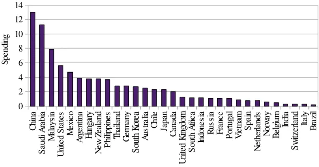
thus, they produce more. Figure 1.1 shows for a set of countries the total value announced to be
spent by the year of 2009 in the so called “rescue packages”. As we can see, governments put a
lot of effort in stimulating the economy, in some cases announcing to spend more than 10% of
GDP. Since a lot of resources are being allocated to those policies, it is important to understand
what is the best way to implement them. In this paper, we explore the dynamic property of
co-ordination failures, trying to answer questions concerning the timing of interventions, such as:
for a budget constrained policy maker, is preventing a crisis better than rescuing the economy
after a crisis has already come? Should policy makers give up early on avoiding a recession?
How should the incentives vary with economic activity and fundamentals?
To answer those questions, we need a model where expected demand is important to
de-termine the outcomes of real variables. In other words, we need a model where “market
con-fidence” plays a role. This is not captured in a model where fluctuations of employment and
capacity utilization are only consequence of price rigidities, but there are models in the
litera-ture where fluctuations of output are explained by changes in expectations. The expectations
about the production level of others might be important to determine the production level of a
given agent, since a higher output implies a higher demand for his product (see Cooper & John
(1988) and Kiyotaki (1988)). Thus, his production level depends on his expectations about
the production of others. Changes in expectations are usually assumed to be driven by some
“sunspot” variable, or simply, in the words of Keynes, by “animal spirits”. Those models
Figure 1.1: 2009 announced fiscal rescue package as % of GDP C hi na S au di A ra bi a M al ay si a U ni te d S ta te s M ex ic o A rg en tin a H un ga ry N ew Ze al an d P hi lip pi ne s Th ai la nd G er m an y S ou th K or ea A us tr al ia C hi le Ja pa n C an ad a U ni te d K in gd om S ou th A fri ca In do ne si a R us si a F ra nc e P or tu ga l V ie tn am S pa in N et he rla nd s N or w ay B el gi um In di a S w itz er la nd Ita ly B ra zi l 0 2 4 6 8 10 12 14 S pe nd in g
Source: adapted from Khatiwada (2009). 2009 GDP based on IMF’s growth forecasts for 2009.
hibit coordination failures, since depending on agents expectations a bad equilibrium can be
played.
Instead of following this strand, we develop a dynamic macroeconomic model where
fluctu-ations are triggered by shocks on productivity, but that keeps the coordination failure aspect (in
the sense that if agents agreed to increase their production everyone would be better off) and the
key role of expectations2. The model features staggered investment decisions and monopolistic competition. Staggered investment decisions are important to keep the key role of expected
demand to determine output, since capital can not adjust overnight to changes in demand. We
apply theoretical results of dynamic games with timing frictions to this macro model, allowing
us to work with an unique equilibrium. Then, we use this model to study the costs of different
interventions that are equally welfare improving.
In our model, a continuum of investors, each one producing a different variety, receive
sequentially investment opportunities, but they are not certain if others will take this opportunity
or not in the future, since they do not know future values of fundamentals. Investment of others
is important to determine the demand for a given product, and therefore, expectations about the
investment decisions of others are important to determine investment decisions today. To clarify,
consider an investor to whom was offered an investment opportunity, for example, importing a
new machine. The same opportunity will be offered sequentially to other investors after some
time. The extra profit generated by investing is increasing in the quantity of investors that will
invest in the future, since this will increase their output and therefore the demand and the price
for a given product. Suppose that if the increase in production resulting of investing is larger
than 10%, then it is a dominant choice to invest, whatever his expectations about the action of
others are. Also, if this number is 5%, then it is not worth to acquire this machine, since it
does not pay its fixed cost even when the others invest and the demand is high. If the additional
production is between 5% and 10%, then an investor’s decision depends on his expectations
about the actions of other investor. There are multiple equilibria in this model, as usual. Now
suppose the investor knows the additional profit generated by acquiring this machine today, but
he is not certain of what it will be in the future (for example, variables such as exchange rate
or weather can affect this). Using the techniques proposed in Frankel & Pauzner (2000) (FP
hereafter) and later generalized in Frankel & Burdzy (2005) (FB hereafter) it can be argued
that those kind of shocks will lead to an unique outcome of the game. More importantly, it
allows us to work with an economy where recessions are triggered by shocks on fundamentals
(instead of relying on multiple equilibria) and the expectations about the actions of others still
play an important role. Moreover, this model is tractable to analyze policy interventions that try
to mitigate coordination failures.
For a given level of economic activity investors take the opportunity if fundamentals are
sufficiently high and do not take otherwise. The higher the production of others today, the
lower the fundamental needed to invest. The equilibrium in our model is characterized by
a cutoff strategy given by a threshold that is a decreasing functions of the fundamentals on
the proportion of investors operating at maximum capacity. Our results suggest that the best
policy is the one that drifts the threshold downwards, not changing its slope, meaning that the
government should not bias incentives towards avoiding crisis or towards taking the economy
out of it.
In recent years, global games have been used to study a wide variety of economic problems
with some kind of strategic complementarity. These models are in some way related to ours. In
the next section we briefly review some related literature. Section 2 presents the model.
Sec-tion 3 presents an approximated version of this model and shows how we solve it numerically.
2
Related Literature
Carlsson & vanDamme (1993) study a two players and two actions game in which for
inter-mediary values of a payoff parameter there are two equilibria. They show that multiplicity does
not persist in an incomplete information environment, where players do not observe this payoff
parameter, but instead, they receive a noisy signal about it. This logic has been extended in
several ways to study different economic problems, providing uniqueness in different
environ-ments, but with similar information structure. The following paragraph gives some examples1. Frankel, Morris & Pauzner (2003) generalize the results of Carlsson & vanDamme (1993)
for games with an arbitrary number of players and actions. Morris & Shin (1998) study a model
of currency attacks where a continuum of speculators must decide whether or not to attack a
peg. Instead of observing directly the shadow exchange rate (that is, the exchange rate that
would prevail in case the peg was abandoned), speculators observe just a noisy signal about
it. Corsetti et al. (2004) extend this model including a large speculator, showing that players
become more aggressive in the presence of this large speculator. Guimaraes & Morris (2007)
analyze in a model of currency attacks with a continuum of actions how players’ risk attitudes,
wealth and portfolio composition can influence their position in a pegged currency. Morris &
Shin (2004) develop a model where a continuum of banks receive a public and a private signal
about fundamentals and must decide if they rollover the debt of a given project, which succeeds
only if a large proportion of banks roll it over. Bebchuk & Goldstein (2011) use this model to
study credit freezes and the impact of different interventions such as guarantees, interest rate
reductions, direct government lending, infusion of capital into banks, etc. Goldstein & Pauzner
(2005) find an unique equilibrium of a model of bank runs similar to the one of Diamond &
Dybvig (1983) in the absence of common knowledge about fundamentals. Sakovics & Steiner
(forthcoming) build a model to address the question of who the government should rescue in
a crisis, suggesting that the government should focus on sectors that have large externality on
others but such that the others have small externalities on it.
These papers previously mentioned deal with static environments and focus on the absence
of complete information to select equilibria in games with strategic complementarity. There is
another strand of the literature that exploits the dynamic structure of some economic problems,
introducing fundamentals varying over time and subject to shocks. There are frictions: once
an agent picks a position, he will be there for some time. Burdzy, Frankel & Pauzner (2001)
build a model where a continuum of players is randomly matched to play a symmetric 2x2
game. Assuming that the payoff matrix changes according to a random walk and that players
get locked in their actions for some time, they prove uniqueness of equilibrium in limiting cases
where either the frictions or the shocks go to zero. FP build a different but related model,
where the fundamentals varies over time according to a Brownian Motion, and players have
to choose a state in which they will be locked in for a while. Their uniqueness result for the
Brownian Motion case does not rely on small frictions or small shocks. FB generalize some of
the results in FP for more general stochastic process, permitting, for example, that it presents
some mean reversion. He & Xiong (2012) characterize an unique threshold equilibrium in a
model of dynamic debt runs related to FP but with different payoff structure. Cheng & Milbradt
(2012) extend this model to study optimal debt maturity, debt policy and “bailouts”. The model
allows managers to risk-shift, choosing a project with higher risk and smaller expected return.
Debt maturity should be an interior solution that does not induce managers to risk-shift in good
times but also that does not make the probability of rollover risk too high. Guimaraes (2006)
builds a dynamic model of speculative attacks and characterize an unique threshold equilibrium
in a model similar to FP but without strategic complementarity.
There are papers in the macroeconomic literature that deal with the role of expectations
on determining economic outcomes. Lorenzoni (2009) develops a model where agents observe
their own productivity and a signal regarding aggregate productivity. Demand shocks in this
model are caused by “mistakes” about aggregate productivity. The paper tries to evaluate how
much of output volatility can be explained by those demand shocks. Blanchard, L’Huillier &
Lorenzoni (2009) explore empirically the task of separating fluctuations due to news shocks
from the ones resulting of noise shocks. Nimark (2012) explores the effect of unusual events
on agents beliefs and their implications to economic variables. The main idea is that observing
a signal about a “man-bites-dog” event (i.e., an unusual event) lowers the uncertainty about
the event, but being aware of the existence of such signal raises the uncertainty. He builds a
information structure that can help to explain some stylized facts, such as persistent periods
of macroeconomic volatility, large changes in macro variables without large changes in
funda-mentals and the positive correlation between macro data and dispersion of expectations. Eusepi
& Preston (forthcoming) introduce learning in a business cycle model, generating periods of
and Angeletos & La’O (2009) study the role of dispersed information in a RBC model. For
in-stance, they show how a large component of fluctuations can be seen as a product of dispersed
information, rather than uncertainty about underlying fundamentals or shocks to real variables.
Broadly speaking, our papers differs from previous literature in some aspects: we emphasize
the role of coordination failures; despite coordination playing a key role, we do not rely on
mul-tiple equilibria to generate cycles; our model does not exhibit dispersed information, neither
uncertainty about the present values fundamentals, fundamentals are common-knowledge; we
3
Model
Time is continuous and there is a continuum of individuals with mass equal to 1. Agents
discount utility at rateρ. We omit time subscripts in this section. Every agent produces a dif-ferentiated good. The instantaneous utility over consumption goods of the agent that produces
the good jis given by
Uj=
Z 1
0
c(i jθ−1)/θdi
θ/(θ−1)
, (3.1)
whereci j is the quantity of good i(that is, the good produced by agenti) consumed by agent j
andθ >1 is the elasticity of substitution. Letyjbe the quantity produced by agent j. Therefore, his budget constraint is
Z 1
0
pici jdi≤pjyj≡wj, (3.2)
wherepiis the price of the good produced by agenti(or, shortly, the price of goodi).
Technology is the following. If an agent is in stateLow he can produce up toyL units. If
he is in stateHigh he can produce up to yH >yL. Individuals get a chance to switch states
according to a Poisson process with arrival rateα. Once an individual is picked up, he has to choose a state and he will be locked in this state until he gets selected again. Choosing state
Lowis costless. Choosing stateHighimplies a disutilityψ. We denote byhthe proportion of agents in stateHigh.
We can interpret choosing stateHighand paying the fixed costψas an investment decision. For example, we can think ofψ as the cost of importing a machine and the differenceyH−yL as the gain in productivity resulting of this machine. The Poisson process addresses the fact
that this machine will become obsolete after some time and also that firms cannot change their
capital level overnight. Another possible interpretation of paying this fixed cost is hiring a
worker, which cannot be fired before his contract expires1. In what follows we will adopt the
first interpretation. This is a simple and tractable way of modeling the fact that there are fixed
costs that must be paid to produce at a lower marginal cost and staggered investment. Those are
the features that our model aims to capture.
LetA>0 be a productivity parameter. We re-parametrize yH andyL, settingxH andxL to
satisfyyH=AxHandyL=AxL. We seta=logAand let the productivity vary on time according
to
dat=η(µ−at)dt+σdZt, (3.3) whereη ≥0, σ >0 and Zt is a standard Brownian motion. The parameterη represents how fast this process returns to its mean, which is given byµ.
3.1
Equilibrium
In any period supply must equal demand, since the goods are non storable. Take an
individ-ual j who has incomewj. Fix an i∈(0,1). Maximizing equation 3.1 subject to equation 3.2,
we find agent’s jdemand for the good produced by agenti
ci j =
wj
P pi
P
−θ
, (3.4)
where
P≡
Z 1
0
p1i−θdi
1/(1−θ)
. (3.5)
Taking integrals of equation 3.4 in the interval(0,1), with respect to j, we get to the total
demand for the goodi, which is given by the left hand side of equation 3.6 below. Therefore,
equation 3.6 is the market clearing condition of the goodi
yi=
pi
P
−θ
Y, (3.6)
where
Y = R1
0 pjyjd j
P . (3.7)
pi=y−
1/θ
i Y1/θP. (3.8)
Now suppose that an individual has chosen not to pay the fixed cost. In this case, we can
show that he will choose to produceyL, since the marginal cost is zero on the interval [0,yL).
Likewise, if he has chosen to pay the fixed cost he will produce as much as possible, that is,yH.
Thus, in equilibrium, agents locked in stateHigh will produce yH and agents locked in state
Lowwill produceyL. Also, there will be two prices on the economy, pH and pL (associated to
production level yH andyL, respectively). Hence, the income available to individuals in each
case is given by
wH= pHyH=y
θ−1
θ
H Y
1/θP (3.9)
and
wL =pLyL=y
θ−1
θ
L Y
1/θP. (3.10)
We can also write
Y =
hy
θ−1
θ
H + (1−h)y
θ−1
θ
L
θθ−1
. (3.11)
Letv(w)be the indirect utility over consumption goods. Maximizing equation 3.1 subject
to equation 3.2 we find thatv(w) =w/P.Thus, combining equations 3.11, 3.9 and 3.10 we get
the instantaneous utility over consumption goods of individuals locked in each state:
u(yH,h) =y
θ−1
θ
H
hy
θ−1
θ
H + (1−h)y
θ−1
θ
L
θ−11
(3.12)
and
u(yL,h) =y
θ−1
θ
L
hy
θ−1
θ
H + (1−h)y
θ−1
θ
L
θ−11
. (3.13)
Let the function π(h,a) be the difference in the instantaneous utility between individuals locked in stateHighand agents locked in stateLow. Thus,
π(h,a) =ea
hx
θ−1
θ
H + (1−h)x
θ−1
θ
L
θ−11
x
θ−1
θ
H −x
θ−1
θ
L
Notice that the functionπ is increasing in bothaandh. The intuition for this result is that whenhis high, the demand for a given variety is high and so is its price. Thus there are strategic
complementarities: the higher the production level of others the higher the incentives for a given
agent to increase his production level. This incentive comes from the demand channel, once the
investment of others increases their production and their income, which in turn increases the
demand for any given variety, raising its price. That is, the price of a given variety depends
on how large is its production relative to other varieties. If its production is much larger than
the others, its relative price is low, and high otherwise. Thus, it might be worth to increase
productivity only if others do so. The fundamental a captures the supply side incentives to
invest, since a largerameans a higher productivity differential between agents who had invested
and those who had not.
An agent at timet =τthat gets a chance to switch states will do so, if, and only if,
Z ∞
τ e
−(ρ+α)(t−τ)E
τ[π(ht,at)]dt ≥ψ. (3.15) That is, if the additional payoff of choosing the stateHighis higher than the fixed cost he has
to pay to be in that state. Notice that besides the discount rate we also discountπ(h,a)with the probability of not getting a new chance to switch states in every period. Notice that investment
decisions depend on expected values ofht, which captures the effect of expected demand on the
payoff of investing. We are assuming that whenever an individual is indifferent between state
HighorLowhe choosesHigh.
A strategy is as a map s(ht,at)7→ {Low,High}. Proposition 1 characterizes conditions
under which we have an unique or multiple equilibria in the case where the fundamental does
not vary over time.
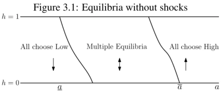
Proposition 1(No Shocks). Assume thatσ=0and a=µ in the initial state. There are strictly decreasing functions aL(h)<aH(h)such that
1. If a<aL(h0)there is an unique equilibrium, in which agents always choose state Low;
2. If a>aH(h0)there is an unique equilibrium, in which agents always choose state High;
3. If aL(h0)<a<aH(h0) there are multiple equilibria, that is, both strategies High and
Low are long-run outcomes.
Figure 3.1: Equilibria without shocks
All choose Low
a h= 1
h= 0 a
All choose High Multiple Equilibria
a
Figure 3.1 illustrates the result of Proposition 1. It shows us that if the productivity differential
is sufficiently high, agents will invest as soon as they get a chance and the economy will move to
a state whereh=1 (and there it will rest). If the productivity differential is sufficiently low, then
it is a dominant choice to never invest, since the gains of investing are offset by the fixed cost. If
the fundamentalais at an intermediary area, then there are no dominant strategies: the decision
to invest or not depends on the expectations about the decision of others. Of course, cycles
are possible in an economy like that, but their existence depends on changes in expectations
and modeling it would require understanding the way agents build their expectations, what can
be quite difficult. Fortunately, as we will see later, we will get an unique equilibrium with
shocks. The cycles will happen not due to changes in expectations about thestrategiesadopted
by others, but instead, by changes in the fundamental of the economy, that will trigger changes
on expectations about theactionsof others in the future.
Now we turn to the general case where the fundamental varies on time. In what follows
we always assume thatσ >0. Proposition 2 below allows us to use the results in FP that will give us an unique equilibrium under some special conditions discussed later in this section. The
same proposition can be proved in a framework that fits the model of FB and it is left to the next
subsection.
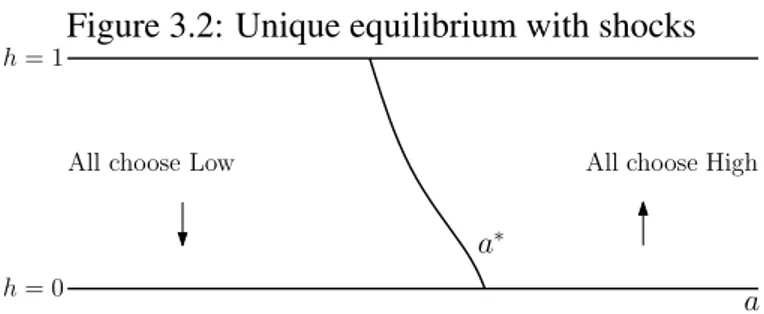
Proposition 2(Shocks). Assumeσ >0. There are constants a′and a′′, with a′<a′′, such that if a>a′′it is strictly dominant to play High and if a<a′it is strictly dominant to play Low.
Proof. See the appendix.
We say that an agent is playing according toa∗(h)if he choosesHighwhenevera>a∗(h)
andLow whenever a<a∗(h). We say that a function a∗(h) is an equilibrium if the strategy
profile where every player plays according to a∗ is an equilibrium. The existence of those
dominance regions proved in Proposition 2 are essential for applying the results of FP and
FB that guarantee existence and uniqueness of the equilibrium, which will be characterized
by a functiona∗(h), although they need extra assumptions. We will discretize this model and
Figure 3.2: Unique equilibrium with shocks
All choose Low
a h= 1
h= 0
All choose High
a∗
The theoretical results underlying the unique equilibrium hypothesis are discussed in the next
section.
We defineV(a,h,a˜) as the gain in utility obtained by choosing High of an agent in state
(a,h)that believes the others will play according to threshold ˜a. That implies that
V(a,h,a˜) = Z ∞
0
e−(ρ+α)tE[π(ht,at)|a,h,a˜]dt−ψ, (3.16) where E[π(ht,at)|a,h,a˜] denotes the expectation of π(ht,at) of an agent in state (a,h) that believes the others will play according ˜a. Although FP and FB prove uniqueness and existence
of the equilibrium, they do not provide a closed solution to the cutoff strategya∗(h)played in
equilibrium2. All we know is that an agent choosing when a=a∗(h) and believing that the others will play the cutoff strategya∗(h)is indifferent between High and Low, which means
thatV(a∗(h),h,a∗) =0, for everyh. Figure 3.2 shows an example of equilibrium in our model.
3.2
Equilibrium Results
If we assume that η=0 we can apply Theorem 1 in FP that states that there is an unique equilibrium in this model. In this equilibrium agents play a cutoff strategy given by a threshold
a∗(h), which means that agents will play High whenever a>a∗(h) and Low whenever a<
a∗(h).
What if η > 0, that is, the movement of a is mean reverting? In that case, FP proved uniqueness only if we consider the limiting cases whereη →0 andσ →0, although the rate at which they go to zero is not important (which means that η can be very large relative to
σ). This will not be the case in our numerical exercises, but we will always assume that the continuous time model presented in this section has an unique equilibrium, even when there is
mean reversion. Why is thisassumptionreasonable? We can justify this in two different ways.
First, in our numerical exercise, with discrete time, we estimated the bounds in which any
threshold that characterize the equilibrium must lie in3. The bounds practically coincided, viding strong evidence that the equilibrium is actually unique. Next section describes the
pro-cedure.
Second, FB generalize the uniqueness and existence results of FP when there is mean
rever-sion, although we would need two extra technical assumptions to apply their results. FB shows
that if we assume thatη is a function of time that asymptotically dies out and that the function
π is Lipschitz inhanda4, the uniqueness is preserved. With this assumption, the environment is not stationary anymore: the strategies that characterize the equilibrium are allowed to vary
over time. But in our discrete model used in the simulations (which will be presented in the
next section) there is no difference in the way we compute payoffs if the mean reversion dies
out after a long time, say 1 billion years, or if the mean reversion remains forever. Thus, for all
practical purposes, we can apply the results of FB looking for stationary thresholds. Below we
discuss more formally the extra assumptions needed and the results of FB.
3.2.1
Relation to Frankel & Burdzy (2005)
Our model can be seen as a special case of FB (and so is the model in FP). In order to apply
the results of FB we should modify it in two different ways. First, the movement ofat should
be given with by equation 3.3, but allowingηt to vary over time in the following way
ηt=
η ift <T
0 otherwise
, (3.17)
whereT is a large number. Also, we assume that the relative payoff is no longerπbut ˆπ instead, where
ˆ
π(h,a) =
π(h,a) ifa<a˜
π(h,a˜) otherwise
, (3.18)
with ˜abeing a large number. One can verify that ˆπ(h,a)is Lipschitz in bothaandh, and contin-uous. In order to apply the results of FB, we have to prove an statement similar to Proposition
2 for this modified (but very similar) model.
Proposition 3. Assume the model is the same of section 3, but with the modifications mentioned
3This is made by eliminating strategies strictly dominated.
above. Ifa is sufficiently high, there are constants a˜ ′and a′′, with a′<a′′ such that if a>a′′ it
is strictly dominant to play High and if a<a′it is strictly dominant to play Low.
Proof. See the appendix.
Proposition 3 guarantees that we can apply the result of Theorem 1 in FB. We state this
theorem here.
Theorem 1. In the model considered in this section, there is an unique outcome that survives
to the iterative elimination of conditionally dominated strategies: for any initial state(a0,h0)
and almost any path of a, the path of h is uniquely determined.
Proof. See FB.
Notice that if ˜aandT are sufficiently large this model is very similar to the previous one.
Moreover, the way we estimate payoffs in the discrete time model will be the same.
3.3
Policies
A policy consists in changing the fixed costψ. We allow this to be state-dependent and thus, a policy is a mapϕ(h,a)that specifies how much the government will pay in each state. There-fore, the fixed cost becomesψ−ϕ instead of justψ. We assume that policies are anticipated by agents.
Since in our model the action of investing has a positive externality on other agents, we
expect that without any intervention there will be underinvestment in this economy. Changing
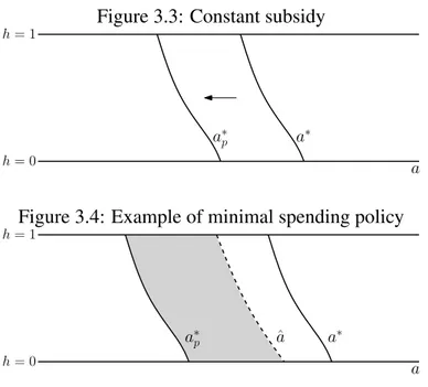
the fixed costψthe policy maker can change the strategy profile played in equilibrium, and thus lead to more or less investment, weakening coordination failures. For example, assume that
government decides to give a constant subsidy, that is,ϕ(h,a) =d>0. Thus, the threshold in equilibrium would drift downwards, froma∗toa∗p, as shown in Figure 3.35. With this threshold there is more investment: for any givenh, agents require a smallerato invest.
But this can be quite expensive: the government is paying subsidies on every possible state.
Of course, an agent choosing whenais very high would not need any incentive to invest. Since
we are dealing with a government that has a finite amount of resources to give out as subsidies,
this policy might not be a good deal.
Figure 3.3: Constant subsidy
a h= 1
h= 0
a∗
a∗ p
Figure 3.4: Example of minimal spending policy
a h= 1
h= 0
a∗
a∗p ˆa
Now we consider a cheaper way in which the government can achieve this same threshold.
Figure 3.4 shows three thresholds: a∗pis the threshold the government wishes to achieve,a∗ is
the threshold without intervention and ˆais the threshold where and agent is indifferent between
HighandLowif he believes that the others will play according toa∗p. Thus playing according
to ˆais the best response of a player that believes the others will play according toa∗p. Assume
that the government commits to give to each player deciding in the gray area a subsidy that is
equal to the relative payoff of investing in that point, given that the others will play according
toa∗p. Thus if he believes that the others will play according to a∗p, playing according toa∗p is
a best response under this policy6. Therefore, the strategy profile where every individual plays according toa∗p is an equilibrium. But notice the equilibrium is no longer unique. If agents
believe that the others will play according toa∗ their best response is to play according toa∗,
and thus, the policy has no effect at all. One possible reason why this multiplicity appears is
that we violated the monotonicity hypothesis of FP: in some areas a higheraleads to a higher
cost, and this can offset the effect on the the relative payoffπ. In fact, we do not even rule out the existence of other weird equilibria. Below we present a formal definition of those policies,
which we callminimal spending policies.
Definition 1. Leta∗ be an equilibrium of the game anda∗p be a continuous function such that
a∗p(h)<a∗(h), for everyh. Let ˆabe the boundary where an agent is indifferent betweenHigh
andLow. We say that the functionϕ(h,a)is the minimal spending policy that implementsa∗pif
ϕ(h,a) =
ψ−R∞
0 e−(ρ+α)tE[π(ht,at)|a,h,a∗p]dt ifa∗p(h)≤a≤aˆ(h)
0 otherwise
. (3.19)
Although the result below is quite intuitive, Proposition 4 formalizes the idea that minimal
spending policies are the cheapest way of achieving a desired threshold.
Proposition 4. Let the threshold a∗be an equilibrium of the game. Let a∗pbe such that a∗p(h)<
a∗(h), a∗p(h)≤aˆ(h)for every h, where is the boundary where V(a,h,a∗p) =0. Let F(a∗
p) be
the family of functionsϕ :[0,1]×R→R+ such that the threshold a∗p is an equilibrium under
the policy given by ϕ. Let ϕm be the minimal spending policy that implements a∗p. Then,
ϕm∈F(a∗p). Moreover,
ϕm=arg min
ϕ∈F(a∗p) Z ∞
0
e−ρtE0ϕ(ht,at)dt
for every initial state(a0,h0). Finally, for every other function ϕ∈F(a∗p)such that {(h,a):
ϕm(h,a)=6 ϕ(h,a)}has positive measure under the belief that the others will play according to
a∗p, we have that
Z ∞
0
e−ρtE0ϕ(ht,at)dt >
Z ∞
0
e−ρtE0ϕm(ht,at)dt.
Proof. See the appendix.
We imposed the hypothesis thata∗p(h)≤aˆ(h)because we do not want to deal with policies
that charge producers, since in our world the government has a fund to stimulate the
econ-omy and it will spend it whenever it wishes. In this work we will compare different minimal
spending policies. We could build policies that achieve the same threshold and guarantee an
unique (threshold) equilibrium, but, of course, they would have to spend more than the minimal
spending policy.
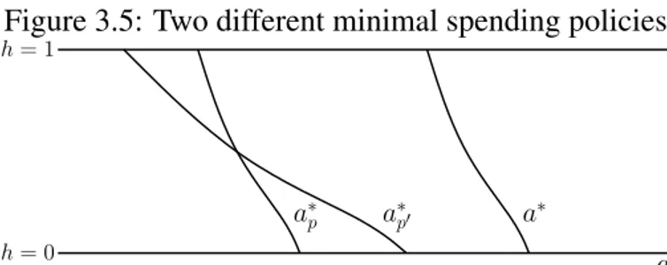
Minimal spending policies are interesting because they are the cheapest way of achieving a
desired threshold. In this work, our aim is to compare different policies that give similar results
in terms of utility gains. We assume that the government has a fixed amount of resources to
stimulate the economy. Then we intend to compare different thresholds that deliver the same
utility and answer the question: what is the cheapest way that government can achieve this level
deliver the same lifetime utility for an agent born in a random state. Our model is capable of
answering which of those policies cost less.
Figure 3.5: Two different minimal spending policies
a h= 1
h= 0
a∗
a∗
4
The Discrete Time Model
In order to solve the model numerically we work with an approximation of the model
pre-sented in section 3. There is still a continuum of individuals with mass equal to 1, but time is
discrete and each period has length∆≈0: timetequals 0,∆, 2∆, 3∆and so on. The stochastic
process ofat is given by
at=at−1+η(µ−at−1)∆+σ
√
∆εt, (4.1)
whereεt are iid shocks with pdf given by the standard normal. In the beginning of each period, afterat is observed,(1−e−α∆)individuals are randomly selected and get a chance to switch
state. The instantaneous payoffs of being locked in each state is the same as before , but now
agents discount their utility by the discount factore−ρ∆t. When∆→0 this model converges to
the model of section 3.
4.1
Threshold Computation
Our algorithm aims at finding a threshold where every agent is indifferent between actions
HighandLowif he believes the others will act according to this threshold. In order to estimate
the relative payoff we assume that time is finite, but sufficiently large. The steps are basically
the following:
1. Pick an arbitrary increasing functiond:R+→R.
2. Pick an arbitrary thresholda∗0and choose a finite grid forhin the interval[0,1].
3. For every point hin the grid, simulate npaths ofat and ht, takinga∗0(h)and has initial conditions of those paths, respectively, and assuming that every agent will act according
4. If the gain in utility is close to zero in every point of the grid, stop. Otherwise, update
a∗0 in the following way: if the payoff at some point (a∗0(h),h) is positive then set an
a∗1(h)<a∗0(h) and if its negative set a∗1(h)>a∗0(h), letting the distance between a∗1(h)
anda∗0(h)be given byd |Vˆ(a∗0(h),h,a∗0)|1
. Go back to step 2, lettinga∗0be given by the linear interpolation of the points(a∗1(h),h), for everyhin the grid.
If after a large number of iterations this procedure did not work, pick another functiondand try
again2.
There is another way to do this, but it turned out to be more expensive in terms of time
needed to compute the threshold. We applied an algorithm similar to the one presented above
to compute the threshold that is a best response of an agent that believes the others will choose
Lowafter him. This best response is characterized by a thresholdaH0. Then, we computed the thresholdaH1 that characterizes the best response of an agent that believes the others will act according toaH0. We repeat this procedure until|anH+1−aHn|becomes sufficiently small. At this point, we take aHn+1 as the equilibrium threshold. This procedure is simply the discrete time counterpart of the iterated elimination of strategies strictly dominated used in the proof of
The-orem 1 in FP. It turns out that if we start the iterations with the best response of a player that
believes the others will playHigh always we practically get to the same threshold as starting
withaH0, which is expected, since our continuous time model (with the extra assumptions pre-sented in subsection 3.2.1) has an unique outcome that survives to the iterated elimination of
strategies strictly dominated and the discrete time model is an approximation of this model. Of
course, those thresholds coincided with the threshold found using the first algorithm presented.
4.2
Policy Simulations
Once we calculated the threshold, we consider some minimal spending policies that could
be implemented. Leta∗ be the threshold calculated using the techniques described in the last
paragraph. Thus we consider policies that try to implement a threshold given by
ac,ξ(h) =a∗(h) +ξ ϑ(h)−c, (4.2)
1In others words, the higher the distance of the payoffs from zero, the higher the change in a. This pro-cedure is equivalent to imposing that the function d is an odd function from R to R and setting a∗1(h) =
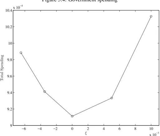
whereϑ(h) =1−2h,c>0 andξ is a real number. We refer to a policy as a pair(ξ,c). We are translating the threshold to the left and then rotating it3. Depending on the values ofξ we are raising or lowering its slope. Initially, we fix a finite grid forξ that includes zero and a value forc. For example we could letξ belong to{−1,0,1}. Then, we estimate the lifetime utility of a representative agent born in a given state, taking out the first 50 years. If it is not the same
for all policies, we change the constantcin each policy (that is, we translate the threshold). We
keep doing this for each policy until we get an utility very close to the policy(0,c). After we
are done we will have many different policies that deliver the same utility but have different
slopes4.
For each policy, we find the gray area in Figure 3.4, that is, we find the best response of an
agent, given that the others will follow the threshold prescribed by the policy. We also compute
the gain in utility of pickingHighof an agent choosing in this area, for a finite set of points. We
will use a couple of linear interpolations to find the gain in utility of choosingHigh of agents
in the gray area but not at this finite set of points. Finally, we simulate the economy several
times and estimate the government spending under each policy by applying the formula given
by equation 3.19, taking averages.
3Like in Figure 3.5.
5
Results
Calibration. We chose parameters such that:
• Applying the two quarters definition of business cycles1, the mean of the GDP in peaks is about 4% higher than it is in troughs;
• The economy stays 30% of time to the left of the threshold, that is, agents are not investing 30% of the time, approximately. We choose the parallel policy such that under that policy
this number falls to 12%.
• Once the economy goes to the left of the threshold, the mean time it stays there is 5 quarters. Here, we say that the economy went to the left of the threshold if it crossed it
and remained there for at least 36,5 days2.
If we think of the economy being in a crisis when to the left of the threshold, our calibration is
simply requiring that the economy is in recession 30% of time, recessions last about 5 quarters
but the GDP does not change too much. Also, in our calibration, if we apply the two quarters
approach to the GDP data we get an economy that is about 50% of time in recession3, with crisis also lasting about 5 quarters4.
It is important to mention the way we compute GDP in the calibration. We assume that
instead of paying the fixed cost all at once, agents pay a “rent” for using the machine that equals
(ρ+α)ψin every period he is locked in stateHigh. An agent is indifferent between paying this rent or payingψ unities of his lifetime utility all at once. Thus GDP in a given period of time is given by equation 3.11 minus(ρ+α)ψ. We do this because a fixed cost payed in an expansion might increase GDP in a recession as well, since it will last for some time, and thus, the cost
should not be all paid in the expansion. One can think of agents taking loans from an external
1It means that a crisis starts when GDP goes down for two consecutive quarters and ends when it goes up for two consecutive quarters.
2For example, it is not reasonable to say that an economy is in a crisis if unemployment fell for 3 consecutive days. That is the reason why we eliminate very temporary crossings.
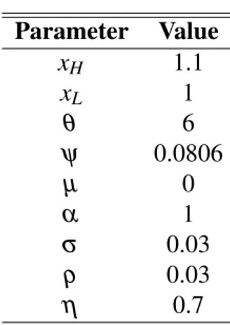
Table 5.1: Parameters
Parameter Value
xH 1.1
xL 1
θ 6
ψ 0.0806
µ 0
α 1
σ 0.03
ρ 0.03
η 0.7
lender to buy the machine. Agents are simply paying the user cost of it, that is, its depreciation
plus an interest.
The parameter µ andxL were normalized to zero and one, respectively. The chosen values of the parametersθ andρ are standard in the literature. α was made equal to 1, meaning that investment decisions are made once a year. All the other parameters in the model were chosen
to match the desired statistics. Table 5.1 shows the parameters (the time unit is years, when
needed).
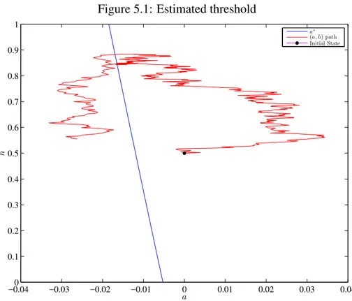
Estimates. Figure 5.1 shows the threshold we estimated, together with a random realization
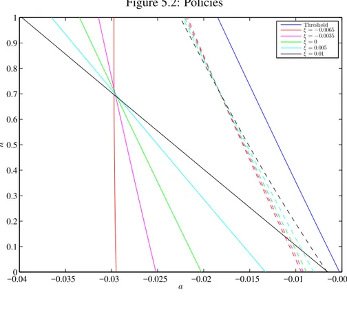
ofat. Figure 5.2 shows the values of ξ chosen and their respective policies. The policies in Figure 5.2 have already been adjusted to deliver all the same utility5. All those policies improve welfare, although the best policy in terms of utility is the one that makes agents invest always
(but it also turns out to be much more expensive than the ones considered here). The dashed
lines are the curves where an agent is indifferent between investing and not investing if he
believes the others will act according to the threshold of same color, and thus, the government
pays subsidies in the area between the policy threshold and this dashed threshold.
Figure 5.2 provides a good intuition of what is going on in each policy. Consider an
econ-omy that got in a crisis, withh=0 and a low value of fundamental, saya=−0.045 in Figure
5.2. Supposeat starts going up towards the mean zero. As soon as he notice the fundamentals
are getting slightly better, the “red policy maker” (the policy maker that implements the
thresh-old with higher slope) begins to stimulate the economy and keeps doing so for a long time. The
“black policy maker” (the policy maker that implements the threshold with lower slope) gives
out stimulus only when the fundamentals are really good and he is almost sure he will not have
to give out stimulus for a long time. The red policy maker puts a lot of effort in taking the
economy out of the crisis, while the black one does not. Now suppose the fundamental is high,
say 0, andh=1 (the economy is in an expansion). Assume the fundamental starts going down
towards−0.045. Both will start giving out incentives almost at the same time, although the red
policy maker starts first. If things keep getting worse, the red policy maker soon give up and let
the economy get in a crisis (waiting things to get slightly better to stimulate it), while the black
policy maker persists, he puts a lot of effort on avoiding the crisis. We say that the black policy
maker is obsessed with preventing crisis, but once they happen he will just act if fundamentals
are really worth. The red policy maker is concerned with taking the economy out of a crisis, but
does not put much effort on preventing it. Moreover, notice that the red policy maker practically
only looks at the fundamental when deciding to stimulate the economy or not.
This discussion highlights that prevention has a cost. For example, maybe the extra effort of
the black policy maker in relation to the red one can be useless: agot so low that the economy
got in a crisis anyway. But maybe, this extra effort was rewarded: the fundamental got better and
he avoided the crisis, while the red one did not, and had to spend anyway to bring the economy
back to high employment, while experiencing a bad time. Maybe less incentives were necessary
to prevent than it is to take the economy out of a crisis, since the strategic complementarity did
not push payoffs down. The same can be said in the opposite direction. Trying to get out of
a crisis at the first opportunity can be useless if the fundamentals return to a low level quickly.
But if the fundamentals went to a no crisis level, then this effort might have been rewarded: the
economy left the crisis earlier (although they probably paid more to get that result). Figure 5.3
shows the subsidies whenh=0 andh=1 in both policies.
For example, notice the value of the subsidy paid by the black policy maker whenh=1 and
a=−0.025 (which he pays to prevent a crisis) is much smaller than the subsidy paid by the red
policy maker whenh=0 anda=−0.025, which he pays to take it out of a crisis (see Figure
5.3). Thus, if fundamentals after a fall got better, probably the red policy maker spent more
to get the economy to full employment. But maybe it was useless and the economy got in a
crisis to both of them. Also, the amount necessary to prevent crisis for the black policy maker is
smaller for the same values of the fundamental, as we can see in Figure 5.3. Since agents know
that whenh=1 the black policy maker will give out stimulus for a longer time, they demand
less incentives to invest. This reinforces our point that avoiding a crisis can be worth, although
still remains the possibility that no effort was necessary.
Figure 5.1: Estimated threshold
−0.04 −0.03 −0.02 −0.01 0 0.01 0.02 0.03 0.04 0
0.1 0.2 0.3 0.4 0.5 0.6 0.7 0.8 0.9 1
a
h
a∗
(a, h) path Initial State
is the one that gets the smaller cost. It indicates too much preventing can be a bad thing, since
sometimes it is not worth to prevent a crisis, it will happen anyway. But so is trying too hard
to take the economy out of a crisis. The government should not bias the incentives towards
avoiding crisis or rescuing the economy. Notice that the parallel policy decide when to pay or
not subsidy according to the distance of the economy from the original threshold. This policy
is equivalent to a policy that gives out a constant subsidy in every state of the world (but it is
Figure 5.2: Policies
−0.04 −0.035 −0.03 −0.025 −0.02 −0.015 −0.01 −0.005 0 0.1 0.2 0.3 0.4 0.5 0.6 0.7 0.8 0.9 1 a h Threshold
ξ=−0.0065
ξ=−0.0035
ξ= 0
ξ= 0.005
ξ= 0.01
Figure 5.3: Subsidies
−0.03 −0.025 −0.02 −0.015 −0.01 −0.005 0 0.2 0.4 0.6 0.8 1
x 10−3
ϕ
(0
,a
)
a
Subsidy withh= 0
ξ=−0.0065
ξ= 0.01
−0.04 −0.038 −0.036 −0.034 −0.032 −0.03 −0.028 −0.026 −0.024 −0.022 −0.02 0 0.2 0.4 0.6 0.8 1
x 10−3
ϕ
(1
,a
)
a
Subsidy withh= 1
ξ=−0.0065
Figure 5.4: Government spending
−6 −4 −2 0 2 4 6 8 10 x 10−3 9
9.2 9.4 9.6 9.8 10 10.2 10.4x 10
−4
ξ
T
ot
al
S
p
en
d
in
6
Conclusion
We built a dynamic macroeconomic model where agents investment decisions have impacts
on other agents, leading to coordination failures. We have shown how this model is capable
of generating cycles, i.e., fluctuations of GDP and capacity utilization (or employment) in an
unique equilibrium environment. In our model, cycles does not rely on changes from one
equi-librium to another, usually assumed to be driven by changes in expectations. Recessions in
our model are triggered by shocks on productivity, but expectations about the actions of others
still play an important role, in the sense that recessions could be avoided if agents were able to
commit to certain strategies.
We used this model to study the impact of different policies that aim to mitigate
coordina-tion failures. Our results suggest that the policy makers should not bias the incentives toward
avoiding crisis or taking the economy out of it. We find out that the best policy is equivalent to
APPENDIX A -- Proofs
Proof of Proposition 1. Assume that an agent has the belief that after he chooses, every
agent that get a chance to change state will choose state Low. That means that he assigns
probability 1 that the path ofht will beht↓=h0e−αt. Thus, choosingHighraises his payoff by
the amount
U(h0,a) =
Z ∞
0
e−(ρ+α)tπ(ht↓,a)dt−ψ
=ea
x
θ−1
θ
H −x
θ−1
θ
L
Z ∞
0
ht↓x
θ−1
θ
H + (1−h↓t)x
θ−1
θ
L
θ1−1
dt−ψ.
(A.1)
Therefore this agent will choose stateHighiffU(h0,a)≥01. SinceU(h0,a)is continuous
and strictly increasing inaand lima→∞U(h0,a) =∞, lima→−∞U(h0,a) =0, we have that for
anyh0there is aa=aH(h0)such thatU(h0,a) =0. SinceU(h0,a)is strictly increasing ina, for
anya′>aH(h0)we haveU(h0,a′)>0 and thus choosing Highis strictly dominant, since any
other belief he might have about the path ofht will raise the relative payoff of choosingHigh.
Notice thatU(h0,a)is strictly increasing in bothaandh0and thusaH(h0)is strictly decreasing.
Applying a similar argument we can prove that there is a thresholdaL(h0)such that ifa<
aL(h0)the dominant choice is to chooseLow and also that this function is strictly decreasing.
To do so, we consider an agent with the belief that others will chooseHigh after him. That
means that he believes that the motion ofhtwill be given byh↑t =1−(1−h0)e−αt. In that case,
choosingHighinstead ofLowraises his payoff by the amount
U(h0,a) =
Z ∞
0
e−(ρ+α)tπ(ht↑,a)dt−ψ
=ea
x
θ−1
θ
H −x
θ−1
θ
L
Z ∞
0
ht↑x
θ−1
θ
H + (1−h↑t)x
θ−1
θ
L
θ1−1
dt−ψ.
(A.2)
Therefore, this agent will choose Low wheneverU(h0,a)<0 and, applying the previous
arguments, we can show that there exists a thresholdaL(h0)such that ifa<aL(h0)the dominant
strategy is to always chooseLowand also thataL(h0)is strictly decreasing. Since for everyh0
we haveht↑>h0>h↓t for everyt>0,U(h0,a)>U(h0,a). This impliesaH(h0)>aL(h0).
Take a pair (a,h0) such that aL(h0)<a<aH(h0). Sincea<aH(h0) we have that if an
agent believes that the path ofhtwill beh↓t thenU(h0,a)<0 and thus his optimal strategy is to
playLow. Therefore this belief is consistent and the strategy profile where every player plays
Lowis an Nash equilibrium. Applying the same argument, we can show that sincea>aL(h0)
the strategy profile where every player playsHighis also a Nash equilibrium. Hence, there is
multiplicity in this set.
Proof of Proposition 2. Take an agent deciding at periodτ (which we normalize to zero), withh0=1 and with the belief that the others will chooseHighafter him, that is, he believes
thatht=1, for everyt ≥0. Under this belief, the gain in utility is given by
U(h0,a) =xH
x
θ−1
θ
H −x
θ−1
θ L E0 Z ∞ 0
e−(ρ+α)tE0{eat}dt−ψ. (A.3)
Solving the stochastic differential equationdat=η(µ−at)dt+σdZt we get that
at=a0e−ηt+µ(1−e−ηt) +σ
Z t
0
eη(s−t)dZs. (A.4)
And thusat conditional ona0is normally distributed with
E0[at] =µ+e−ηt(a0−µ) (A.5)
and
Var0[at] =
σ2
2η 1−e
−2ηt
. (A.6)
Thereforeeat conditional ona
0follows a log-normal distribution with
E0[eat] =exp
µ+e−ηt(a0−µ) +
1 4
σ2
η 1−e
−2ηt
. (A.7)
Notice that lima0→−∞E0[e
at] =0.Thus there is anda′ such thatU(l
0,a)<0 and thus it is
Now assume that an agent is deciding under the belief thatht=0 for everyt≥0. Thus his
gain in utility of choosingHighis given by
U(h0,a) =xL
x
θ−1
θ
H −x
θ−1
θ L E0 Z ∞ 0
e−(ρ+α)tE0[eat]dt−ψ.
Since lima0→−∞E0[e
at] =∞, we have that there is a constanta′′such that choosingLowis
strictly dominant to the left ofa′′. Of course,a′<a′′, otherwise we would have a contradiction.
Before we prove Proposition 3, it is useful to establish the following result.
Lemma 1. Let ˆat be the following latent variable
ˆ
at =
at if at <a˜
˜
a otherwise
, (A.8)
where atis given by dat=ηt(µ−at)dt+σdZt, withηtgiven by equation 3.17. Thenlimaτ→∞Eτ
eaˆt= ea˜andlimaτ→−∞Eτ
eaˆt=0, for every t>τ.
Proof. First assume thatτ<T. We know that ifτ<t<T,at|aτ has a normal distribution with
mean and variance given by equations A.5 and A.6, respectively. Thus, in that case we have
Eτeaˆt= 1 Σt
√
2π
Z a˜
−∞
exp
(
at− 1 2
at−µ−e−ηt(aτ−µ) Σt
2)
dat
+
1−Φ
˜
a−µ−e−ηt(aτ−µ) Σt
ea˜, (A.9)
whereΦis the standard normal distribution andΣt≡σ
q
1
2η(1−e−2ηt).
Now fixt≥T. In that case, we have thatat|aT follows a normal distribution with meanaT
and varianceσ2(t−T). Therefore, by the law of iterated expectations,
Eτ[at] =Eτ[Eτ[at|aT]] =Eτ[aT] =µ+e−ηT(aτ−µ), (A.10)
where the last equality follows from equation A.5. Moreover,
We can show thatat|aτ follows a normal distribution2and thus
Eτeaˆt=
1
q
σ2(t−T) +Σ2
T
2π
Z a˜
−∞ exp
at− 1 2
at−µ−e−ηT(aτ−µ)
q
σ2(t−T) +Σ2
T 2 dat +
1−Φ
˜
a−µ−e−ηT(aτ−µ)
q
σ2(t−T) +Σ2
T
ea˜. (A.12)
Notice that both equations A.9 and A.12 are continuous on aτ and that they coincide at
t=T. Taking limits withaτ→∞andaτ→ −∞of equations A.9 and A.12 completes the proof
for the case where τ <T. The proof for the case where τ ≥T is very similar and therefore omitted.
Proof of Proposition 3. We start noticing that ˆπ(h,a) =π(h,aˆ). Therefore, we can apply a proof similar to the one of Proposition 2 together with Lemma 1, assuming that ˜ais sufficiently
high. That is, now we have that the gain in utility of choosingHigh for an agent deciding at
some periodτ and believing thatlt =0 for everyt>τis
U(lτ,a) =xL
x
θ−1
θ
H −x
θ−1
θ L Eτ Z ∞ τ e
−(ρ+α)t
Eτeaˆtdt−ψ.
Thus, since limaτ→∞Eτeaˆt=ea˜, if ˜ais sufficiently high there is an a′′τ such that it is strictly
dominant to playHighto the right of it. But notice thata′′τ does not need to depend onτifτ>T, since the environment is stationary in this case. Therefore, we seta′′ =sup{a′′τ : 0≤τ≤T}. The proof fora′is similar but using the fact that limaτ→−∞Eτ
eaˆt=0.
Proof of Proposition 4. We first show that ϕm ∈F(a∗p), that is, the minimal spending actually implementsa∗p. Ifa∗pis such thata∗p(h)<a∗(h), for everyh, we have that the boundary
(denoted by ˆa) where an agent is indifferent between states High andLow if he believes that
others will play according toa∗pmust lie entirely to the left ofa∗, since the functionπ is strictly increasing in both arguments. Notice that ˆais a best response for a player believing the others
will play according toa∗p. The minimal spending policy raises the utility of agents that believe
the others will play according toa∗p in the area between ˆa and a∗p in the amount necessary to
2We used a known result to prove it. We know that a
T|aτ ∼N(µ+e−ηT(aτ−µ),σ
2
2η(1−e−2ηT)) and at|aT,aτ∼N(aT,(t−T)σ2). SinceEτ[at|aT]is linear onaT andVarτ[at|aT]does not depend onaT we guarantee bivariate normality of the vector(at,aT)conditional on aτ (see Arnold, Castillo & Sarabia (1999), p. 56) and