Factors Affecting the Technical Efficiency of Production
of the Brazilian Banking System: A Comparison of Four
Statistical Models in the Context of Data Envelopment
Analysis.
Geraldo da Silva e Souza
Benjamin Miranda Tabak
March 26, 2003
Abstract
This paper uses an output oriented Data Envelopment Analysis (DEA) measure of
technical efficiency to assess the technical efficiencies of the Brazilian banking system.
Four approaches to estimation are compared in order to assess the significance of
fac-tors affecting inefficiency. These are nonparametric Analysis of Covariance, maximum
likelihood using a family of exponential distributions, maximum likelihood using a
fam-ily of truncated normal distributions, and the normal Tobit model. The sole focus of
the paper is on a combined measure of output and the data analyzed refers to the year
2001. The factors of interest in the analysis and likely to affect efficiency are bank
nature (multiple and commercial), bank type (credit, business, bursary and retail),
bank size (large, medium, small and micro), bank control (private and public), bank
origin (domestic and foreign), and non-performing loans. The latter is a measure of
bank risk. All quantitative variables, including non-performing loans, are measured on
a per employee basis. The best fits to the data are provided by the exponential family
varies according to the model fit although it can be said that there is some
agree-ments between the best models. A highly significant association in all models fitted
is observed only for nonperforming loans. The nonparametric Analysis of Covariance
is more consistent with the inefficiency median responses observed for the qualitative
factors. The findings of the analysis reinforce the significant association of the level of
bank inefficiency, measured by DEA residuals, with the risk of bank failure.
1
Introduction
The main objective of this paper is to compute measures of technical efficiency based
on Data Envelopment Analysis (DEA) for the Brazilian banks and to relate the
vari-ation observed in these measurements to covariates of interest. This associvari-ation is
investigated in the context of four alternative models fit to DEA residuals. The DEA
residuals are derived from a single output oriented DEA measure obtained under the
assumption of variable returns to scale. This approach explores Banker (1993) and
Souza (2001) results for the univariate production model.
The causal factors considered here are bank nature, bank type, bank size, bank
control, bank origin and risky loans (nonperforming loans). Output is measured as
a combined index formed by investment securities, total loans and demand deposits.
The three input sources are labor expenses, capital and loanable funds. All production
variables are normalized by an index of personnel.
2
Data Envelopment Analysis Production
Mod-els
Consider a production process withnproduction units (banks). Each unit uses variable quantities ofm inputs to produce varying quantities of sdifferent outputsy.
Denote by Y = (y1, . . . , yn) the s×n production matrix of the n banks and by
X= (x1, . . . , xn) them×n input matrix. Notice that the element yr≥0 is thes×1
is strictly positive). The matrices Y = (yij) and X = (xij) must satisfy: Pipij > 0 and P
jpij > 0 where p is x or y. The output vector y as well as the input vector x need not in general to be measured in physical quantities.
In our application s= 1 and m = 3 and it will be required xr >0 (which means that all components of xr are strictly positive).
Definition 2.1: The measure of technical efficiency of production of bank ounder the assumption of variable returns to scale and output orientation is given by the solution
of the linear programming problem Maxφ,λφ subject to the restrictions 1. λ= (λ1, . . . , λn)≥0 and Pni λi= 1.
2. Y λ≥φyo. 3. Xλ≤xo.
Suppose that the production pairs (xj, yj), j = 1, . . . , n for the n banks analyzed satisfy the deterministic statistical model yj = g(x)−ǫj, where g(x) is an unknown continuous production function, defined on a compact and convex setK. We assume
g(x) to be monotonic and concave. The functiong(x) must also satisfyg(xj)≥yjfor all j. The quantities ǫj are inefficiencies which are independently distributed nonnegative random variables.
One can use the observations (xj, yj) and Data Envelopment Analysis to estimate
g(x) only in the set
K∗=
x∈K;x≥
n
X
j=1
λjxj, λj ≥0, n
X
j=1
λj = 1
.
For x∈K∗ the DEA production function is defined by
g∗
n(x) = sup
X
j
λjyj;
X
j
λjxj ≤x
,
where the sup is restricted to nonnegative vectorsλsatisfying Pn
j=1λj = 1.
For each banko,gn(xo) =φ∗oyo, where φ∗o is the solution of the linear programming problem of Definition 2.1.
The function g∗
3
Statistical Inference
It is shown in Souza (2001) that gn(x) is strongly consistent for g(x) and that the estimated residuals ǫ∗
nj = (1−φr)yj have approximately, in large samples, the same behavior as theǫj.
Souza (2001) also discusses two family of distributions for the ǫj consistent with the asymptotic results cited above. The gamma and the truncated normal. Since
some of theǫ∗
nj in the sample will be exactly zero the general gamma family cannot be
estimated by standard likelihood methods. It is possible however to fit the exponential
distribution.
Let z0, . . . , zq be variables (covariates) we believe to affect inefficiency. Based on
Souza (2001) results the following two statistical models can be used to fit the
ineffi-ciencies ǫ∗
nj under the assumptions of the deterministic model.
Firstly one may postulate the exponential densityλjexp(−λjǫ) whereλj = exp(−µj) withµj =z0jδ0+. . .+zqjδq. Thezij are realizations of theziand theδi are parameters
to be estimated.
Secondly one may consider the model ǫ∗
j =µj+wj where wj is the truncation at
−µj of the normal N(0, σ2). This model is inherited from the analysis of stochastic frontiers and is equivalent to truncations at zero of the normals N(µj, σ
2
).
For the exponential distribution the mean of the jth inefficiency error is exp(µj) and the variance exp(2µj). For the truncated normal the mean is µj +σξj and the variance
σ2
1−ξj
µ
j
σ +ξj
where
ξj =
φ(µj/σ) Φ(µj/σ)
φ(.) and Φ(.) being the density function and the distribution function of the standard normal, respectively.
These expected values can be used to obtain predicted values for inefficiencies and
therefore to measure goodness of fit for the respective models. One such measure is
the rank correlation coefficient between observed and predicted values.
The modeling alternatives presented here involving the families of exponential and
truncated normal distributions may be justified with the deterministic production
model. However, even if one is not willing to assume an underlying univariate
de-terministic production model, those two families of densities are reasonable model
alternatives and (hopefully) flexible enough to model the distribution of theǫ∗
nj.
Stan-dard maximum likelihood estimation based on random samples will be granted if there
is not strong evidence against independence of the ǫ∗
nj across the units forming the
sample. This latter assumption may be checked by means of the runs test (Wonnacot
and Wonnacot, 1990).
Under the assumption of uncorrelated residuals two other models have been used
in the statistical analysis of inefficiency measures: the Analysis of Covariance (Coelli,
Rao, and Battese, 1998) and the Tobit regression (McCarty and Yaisawarng, 1993).
The Analysis of Covariance model used here has the nonparametric formulation
(Connover, 1998)
rj =z0jδ0+. . .+zqjδq+uj
whererj is the rank ofǫnj and theuj are iid normal errors with mean zero and variance
σ2
.
The Tobit model is formulated as
ǫ∗
nj =
z0jδ0+. . .+zqjδj+uj if ǫj >0
0 if ǫj ≤0
As before the uj are iid normal random variables with mean zero and constant varianceσ2
.
As pointed out in McCarty and Yaisawarng(1993), the Tobit model is adequate
when it is possible for the dependent variable to assume values beyond the truncation
point, zero in the present case. They argue that this is the case in the DEA analysis.
Their wording on this matter is as follows. It is likely that some banks (hypothetical)
might perform better than the best banks in our sample. If these unobservable banks
could be compared with a reference frontier constructed from the observable banks,
they would show efficiency scores greater than unity (over efficiency). This would lead
4
Specification of Inputs and Outputs
In this paper we follow the intermediation approach. Under this approach banks
function as financial intermediaries converting and transferring financial assets
be-tween surplus units and deficit units. In this context we take as output the vector
y= (securities,loans,demand deposits). This output vector is combined into a single measure, also denoted byy, representing the sum of the values of investment securities , total loans and demand deposits. Here we follow along the lines of Sathie (2001)
who, in a similar study of the Australian banking industry, considers demand deposits
as output. All output variables, as shown below, are measured on a per employee
basis since they are normalized by the number of employees. This approach has the
advantage of making the banks more comparable through the reduction of variability
and of the influence of size in the DEA analysis.
We should emphasize here that DEA is quite sensitive to the dimension and
com-position of the output vector. See for Tortosa-Ausina (2002). Our experience indicates
that a more robust measure of technical efficiency is achieved combining the output.
The inputs are labor (l) measured by labor costs, the stock of physical capital (k) which includes the book value of premises, equipments, rented premises and equipment
and other fixed assets, and loanable funds (f) which include, transaction deposits, and purchased funds. Input variables, like the output, are also normalized by the number
of employees.
The data base used is COSIF, the plan of accounts comprising balance-sheet and
income statement items that all Brazilian financial institutions have to report to the
Central Bank on a monthly basis.
The statistical analysis carried out in this paper is restricted to the year of 2001.
Output and input variables are treated as indexes relative to a benchmark. In this
paper the benchmark for each variable, whether an input, an output or a continuous
covariate, was chosen to be the median value of 2001. Banks with a value of zero for
l,k orf were eliminated from the analysis.
Output, inputs, and the continous covariate were further normalized through the
division of their indexes by an index of personnel. The construction of this index
the number of employees by its median value in 2001 (December).
Banks with the y employee normalized values greater than 100 were considered extreme outliers and eliminated from the analysis.
The covariates of interest for our analysis - factors likely to affect inefficiency, are
nonperforming loans (q), bank nature (n), bank type (t) , bank size (s), bank control(c) and bank origin (o). Nonperforming loans is a continuous variate and it is also measured on a per employee basis. All other covariates are categorical. The variable nassumes one of two values (1 - commercial, 2 - multiple), the variable t assumes one of four values (1 - credit, 2 - business, 3 - bursary, 4 - retail), the variable s assumes on of four values (1 - large, 2 - medium, 3 - small, 4 - micro) the variable c assumes one of two values (1 - private, 2 - public) and the variable o assumes one of two values (1 -domestic, 2 - foreign). There is a bank (Caixa Econˆomica Federal - CEF) in the data
base that requires a distinct classification due to its nature. Bank nature for this sole
case was coded 3. Dummy variables were created for each categorical variable. They
are denotedn1, n2, n3, t1, . . . , t4, s1, . . . , s4, c1, c2,and o1, o2 respectively.
5
Data Analysis
We begin the presentation in this section reproducing the table of descriptive statistics
(Table 1). The variable of interest is the output oriented DEA measure of technical
efficiency obtained under the assumption of variable returns to scale.
Looking at the medians it should be noticed that the most striking differences are
observed for bank control were private banks dominate public banks and bank type
were credit institutions dominate. These exploratory findings will aid in the choice of
the best model fitting theǫ∗
nj.
Several publications dealing with applications of DEA in banking and other areas
make use of DEA efficiency measures as dependent variables in regression problems.
Typical examples are provided by Coelli, Rao, and Battese (1998), Eseinbeis,
Fer-rier, and Kwan (1999), and Sathye (2001). These applications typically assume that
efficiency measures are uncorrelated. This assumption is justified for the univariate
deterministic production model in Banker (1993) under the assumption of
Variable Level n Median Mean Std Error
bank nature commercial 24 0.598 0.574 0.064
multiple 103 0.508 0.531 0.030
bank type credit 42 0.641 0.587 0.050
business 41 0.469 0.501 0.045
bursary 13 0.554 0.593 0.074
retail 32 0.508 0.487 0.056
bank size large 18 0.554 0.510 0.062
medium 41 0.542 0.535 0.049
small 28 0.539 0.564 0.059
micro 41 0.554 0.525 0.050
bank control private 113 0.586 0.567 0.028
public 15 0.190 0.293 0.080
bank origin foreign 47 0.577 0.560 0.044
domestic 81 0.500 0.521 0.035
Variable n Runs z p-value
ǫ∗
n 128 65 0 0.500
Table 2: Runs test for response variable. Under the null hypothesis of randomness the
number of runs is normal with mean 65 and variance 31.75.
out heteroscedasticity, in Souza (2001). In the latter case one may use a different
trun-cated normal or exponential distribution for each cross sectional unit. Banker (1993)
suggests that these results may be extended to multiple outputs but the nature of the
production model may require deep changes.
A deterministic production model imposes a restrictive behavior in banking since no
random error is allowed in the model specification. If one uses DEA as a performance
measure not necessarily associated to a theoretical production model the hypothesis
of no correlation should be inspected. Here in order to find evidence against this
assumption we perform a runs test (Wonnacott and Wonnacott, 1990). The results are
shown in Table 2.
It is seen from Table 2 that the null hypothesis of randomness (independence) is
not rejected.
5.1
Statistical Models to Assess the Effects of Covariates
To investigate the effect of bank nature, bank type, bank size, bank control, bank
origin and nonperforming loans on the inefficiency of Brazilian banks we model the
distribution of the inefficiencies ǫ∗
nj as truncated normals and exponentials, and the
inefficiencies themselves as a linear regression and as a Tobit normal model.
To fit the truncated normal, the exponential and the Tobit model we use maximum
likelihood methods.
The presence of potential outliers and heteroscedasticity in the data calls for a
nonparametric Analysis of Covariance with the regression approach. This is achieved
using ranks of the ǫ∗
nj as dependent variables.
The log likelihood for the exponential distribution is given by
128
128
X
j=1
ln (λj)−
128
X
j=1
where
λj = exp{−µj} and
µj =a0+a1n1i+a2n2j+b1t1j+b2t2j+b3t3j+c1s1j+c2s2j+c3s3j+d1c1j+e1o1j+f1qj
In the above expressionsy∗
j =ǫ∗nj, the xij, wherex=n, t, s, c, o, are realizations of the corresponding dummy variables and theqj are realizations of the nonperforming loans variableq. The quantities al, bl, cl, d1, e1,and f1 are parameters to be estimated.
For the truncated normal distribution the log likelihood is
−64 ln2πσ2−
128
X
j=1
ln (hj)−1/2
128
X
j=1
difj
where
difj = (y∗
j −µj)2
σ2
and
hj = Φ
µ
j
σ
.
Notice thatσ2
must also be estimated and that Φ(x) is the distribution function of the standard normal.
For the Tobit model the likelihood function can be seen in Johnston and Dinardo
(1997). It is given by
Y
j:y∗ j=0
1−Φ
µ
j
σ
Y
j:y∗ j>0
1
√
2πσ2 exp
" −(y
∗
j −µj)2 2σ2
#
whereσ is the standard deviation of the normal error component of the model. The Analysis of Covariance has the standard form
rj =µj+uj
where therj are the ranks of theyj∗ and theuj are iid homoscedastic normal errors. We compare the exponential and truncated normal distributions. Optimization was
in SAS v8.2 and the method of Newton-Raphson. The Tobit model was fit with the
same technique using E-Views 4.1.
Table 3 shows the goodness of fit of each model measured as a rank correlation
between observed and predicted values. The correlation is not strong for any of the
models. The best performance is for the maximum likelihood fit of a family of
expo-nential distributions followed closely by the nonparametric Analysis of Covariance.
Model Rank Correlation
Analysis of Covariance 0,439
Truncated Normal 0,151
Exponential 0,471
Tobit 0,273
Table 3: Goodness of fit measures - SAS output.
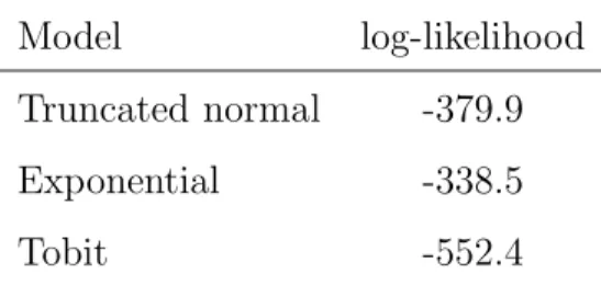
Table 4 shows the log-likelihood of each model fitted by maximum likelihood. These
values seem to be in agreement with the results displayed in Table 3.
Model log-likelihood
Truncated normal -379.9
Exponential -338.5
Tobit -552.4
Table 4: Model log-likelihood - SAS and Eviews(Tobit) outputs.
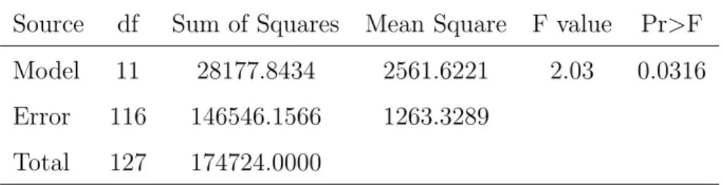
The analysis of variance table for the Analysis of Covariance is shown in Table 5.
The model is significant at the 5% level.
The nonparametric Analysis of Covariance is the model with the highest level of
agreement with the observed behavior of the factor level medians shown in Table 1.
The test statistics of all factor effects are shown in Table 6.
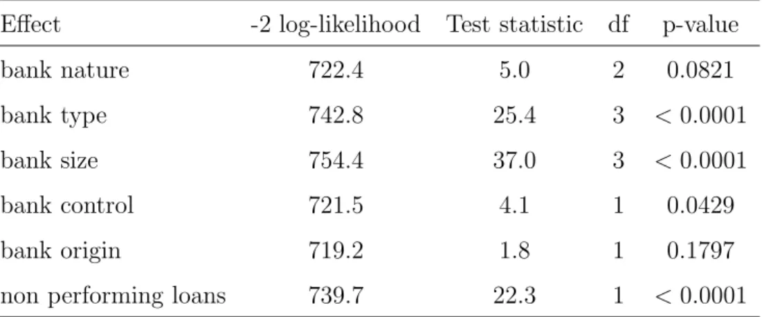
Tables 7 and 8 show the results for the exponential fit. Significance of factor
effects point to the same direction in the nonparametric Analysis of Covariance and the
Source df Sum of Squares Mean Square F value Pr>F
Model 11 28177.8434 2561.6221 2.03 0.0316
Error 116 146546.1566 1263.3289
Total 127 174724.0000
Table 5: Nonparametric Analysis of Covariance - SAS output.
Source df Sum of Squares Mean Square F Pr>F
Nature 2 285.0693 142.5346 0.11 0.8934
Type 3 10928.3752 3642.7917 2.88 0.0388
Size 3 3026.7621 1008.9207 0.80 0.4971
Control 1 6594.3215 6594.3215 5.22 0.0241
Origin 1 695.0160 695.0160 0.55 0.4598
Nonperforming loans 1 18260.6870 18260.6870 14.45 0.0002
Table 6: Significance of factor effects - Analysis of Covariance - SAS output.
size that is significant in the exponential analysis but is not detected in the Analysis
of Covariance. Table 1 favors the latter.
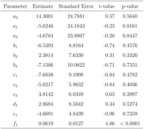
For the sake of completeness I show in Tables 10 and 11 the fit of the truncated
normal and the Tobit. They are consistent to each other in the sense that the only
significant factor is nonperforming loans. It is worth to mention here that the change
of error distribution in the Tobit model did not improve the fit.
6
Summary and Conclusions
Output oriented efficiency measurements, calculated under the assumption of variable
returns to scale, in the context of Data Envelopment Analysis were investigated for
Brazilian banks. In this analysis bank outputs (investment securities, total loans and
demand deposits) are combined to produce a univariate measure of production. The
resulting output is normalized by the median. The same procedure is applied to inputs
Parameter Estimate Standard Error z-value p-value
a0 -1.0032 1.4967 -0.67 0.5039
a1 3.3544 1.3511 2.48 0.0143
a2 3.7245 1.4364 2.59 0.0106
b1 -1.4966 0.3269 -4.58 <0.0001
b2 -0.3379 0.3475 -0.97 0.3326
b3 -1.7023 0.4477 -3.80 0.0002
c1 -2.8303 0.4316 -6.56 <0.0001
c2 -0.6402 0.2996 -2.14 0.0345
c3 -0.4452 0.3913 -1.14 0.2573
d1 0.7998 0.3842 2.08 0.0394
e1 -0.3912 0.2977 -1.31 0.1912
f1 0.0078 0.0018 4.29 <0.0001
Table 7: Exponential Model - SAS output.
Effect -2 log-likelihood Test statistic df p-value
bank nature 722.4 5.0 2 0.0821
bank type 742.8 25.4 3 <0.0001
bank size 754.4 37.0 3 <0.0001
bank control 721.5 4.1 1 0.0429
bank origin 719.2 1.8 1 0.1797
non performing loans 739.7 22.3 1 <0.0001
Parameter Estimate Standard Error t-value p-value
a0 -77.4275 272.51 -0.28 0.7768
a1 -53.4046 268.54 -0.20 0.8427
a2 -18.3174 266.87 -0.07 0.9454
b1 -54.4252 70.14 -0.78 0.4392
b2 71.2125 60.78 1.17 0.2435
b3 -30.3106 80.84 -0.37 0.7083
c1 -79.5144 79.41 -1.00 0.3186
c2 -36.4302 43.77 -0.83 0.0345
c3 62.6940 39.47 1.59 0.4068
d1 -27.8812 58.71 -0.47 0.1147
e1 -88.8044 37.75 -2.35 0.6362
f1 0.2461 0.06 4.17 0.0202
σ2
1029.66 157.84 6.52 <0.001
Parameter Estimate Standard Error t-value p-value
a0 14.3001 24.7881 0.57 0.5640
a1 -5.6246 24.1843 -0.23 0.8161
a2 -4.6784 23.8867 -0.20 0.8447
b1 -6.5493 8.8164 -0.74 0.4576
b2 2.3814 7.6330 0.31 0.3326
b3 -7.1506 10.0822 -0.71 0.7551
c1 -7.6838 9.1998 -0.84 0.4782
c2 -5.0217 5.9632 -0.84 0.4036
c3 3.8142 6.0349 0.63 0.3997
d1 2.8684 8.5042 0.34 0.5274
e1 -4.6691 4.8439 -0.96 0.7359
f1 0.0619 0.0127 4.86 <0.0001
Table 10: Tobit Model - E-Views output.
output and inputs is carried out measuring these variables on a per employee basis.
The number of employees of each bank is also divided the median before this final
normalization. The year of analysis is 2001.
The response variable of interest is defined subtracting from the DEA output
pro-jections the actual output observations. This is the inefficiency error of Banker (1993)
and Souza (2001). The errors thus defined as well as the technical efficiency
mea-surements themselves seem to be independently distributed and, in this context, allow
estimation with the use of regression like methods. Four models were fitted in this
context. Using likelihood procedures, families of exponential and truncated normal
distributions were fit following Banker (1993) and Souza (2001) suggestions. The
To-bit normal regression with truncation at zero which is somewhat popular in the DEA
literature was also tried. Finally a nonparametric Analysis of Covariance was carried
out.
The main objective in fitting a regression like equation to the DEA inefficiency
candidates in this regard here are bank nature, bank type, bank size, bank control,
bank origin, and nonperforming loans.
None of the models used showed a particularly impressive fit, judging by the
corre-lation between observed and predicted values. The best results are for the exponential
distribution and the nonparametric Analysis of Covariance. Significance of factors
however, do not agree 100% in both models. The likelihood analysis of the exponential
fit indicates that bank control, bank size, bank type and non performing loans are
significant effects. Bank nature is marginally significant. Bank nature and bank size
are not significant in the Analysis of Covariance. The analysis of covariance results are
closely related to the median responses of technical efficiencies for each factor.
From a pure descriptive point of view the most striking feature in regard to tables of
efficiency by factor effect levels is furnished by bank control. Private banks are almost
twice as efficient as public banks in the mean and about three times as efficient in the
median. As expected this impression is also captured by the Analysis of Covariance
where the factor Control is seen to be the most signifficant effect.
All models indicate a strong association between risk and efficiency measures. The
rank correlation between these two measurements is 0.594, significantly distinct from
7
References
Banker, R. D. (1993), Maximum likelihood consistency and DEA: a statistical
foun-dation, Management Science, 39(10):1265-1273.
Coelli, T., Rao, D. S. P. and Battese, G. E. (1998),An Introduction to Efficiency and
Productivity Analysis, Kluwer, Boston.
Eseinbeis, R. A., Ferrier, G. D. and Kwan, S. H. (1999), The Informativeness of
Stochastic Frontier and Programming Frontier Efficiency Scores: Cost Efficiency
and Other Measures of Bank Holding Company Performance, Federal Reserve
Bank of Atlanta, Working paper 99-23.
Jhonston, J. and Dinardo, J. (1997),Econometric Methods, 4th ed, McGrawhill. New
York.
McCarthy, T. A. and Yaisawarng, S. (1993), Technical efficiency in New Jersey school
districts, in The Measurement of Productive Efficiency, Oxford University Press,
New York.
Sathye, M. (2001), X-efficiency in Australian banking: an empirical investigation,
Journal of Banking and Financing 25, 613-630.
Tortosa-Ausina, E. (2002), Bank cost efficiency and output specification, Journal of
Productive Analysis, 18, 199-222.
Souza, G. S. (2001), Statistical properties of data envelopment analysis estimators of
production functions, Brazilian Journal of Econometrics, 21(2):291-322.
Wonnacott, T. H. and Wonnacott, R. J. (1990), Introductory Statistics for Business