Efficiency and integration in European banking markets

(1)

Carlos Pestana Barros & Nicolas Peypoch

A Comparative Analysis of Productivity Change in Italian and Portuguese Airports

WP 006/2007/DE _________________________________________________________

Cândida Ferreira

Efficiency and integration in European banking

markets

WP 08/2011/DE/UECE _________________________________________________________

Department of Economics

W

ORKING

P

APERS

ISSN Nº 0874-4548

School of Economics and Management

(2)

Efficiency and integration in European banking markets

Cândida Ferreira[1]

Abstract

This paper seeks to contribute to the relatively scarce published research on the relationship between bank efficiency and European integration in the wake of the recent financial crisis. Using Stochastic Frontier Analysis and Data Envelopment Analysis approaches, the study estimates bank efficiency for different panels of European Union countries during the time period 1994-2008. The main conclusions point to the persistence of inefficiencies, which decreased with the implementation of the European Monetary Union (in the time period 2000-2008) but then increased slightly in the most recent phase (2004-2000-2008), during which the EU had to adapt to the new universe of 27 member-states. On the other hand, there is evidence of a convergence process, although this is very slow and not strong enough to avoid the differences in the country efficiency scores.

[1]

ISEG-UTL - Instituto Superior de Economia e Gestão – Technical University of Lisbon and UECE – Research Unit on Complexity and Economics

Rua Miguel Lupi, 20, 1249-078 - LISBOA, PORTUGAL tel: +351 21 392 58 00

(3)

Efficiency and integration in European banking markets

1. Introduction

The European banking institutions play a unique role in the context of the European Monetary

Union, as the increase of competition in all financial-product market segments is expected to

contribute to price and cost reductions and benefit the exploitation of scale economies.

In recent years, financial systems have been experiencing the consequences of the strong

imbalances and turbulence caused by the US sub-prime mortgage market, which affected

different segments of the international money and credit markets and revealed the fragility of

many financial institutions, including some EU banking institutions and markets.

The ensuing crisis drew attention to the importance of studies seeking to identify the factors

explaining the weaknesses in the financial systems at national and international levels. There

is already a large strand of literature on the analysis of the determinants of efficiency and

particularly on the empirical measurement of the profit and cost efficiency in banking (among

others, Altunbas et al., 2001; Goddard et al. 2001, 2007; Williams and Nguyen, 2005;

Kasman and Yildirim, 2006; Barros et al. 2007; Berger, 2007; Hughes and Mester, 2008;

Sturm and Williams, 2010).

Nevertheless, in Europe there is no clear consensus on the evidence of increasing

consolidation and integration of the European markets. Some empirical studies conclude that

there is evidence of integration, particularly of the European money market, but also to some

extent of the bond and equity markets (Cabral et al., 2002; Hartmann et al., 2003; Guiso et al.,

2004; Manna, 2004; Cappiello et al., 2006; Bos and Schmiedel, 2007). Other empirical

(4)

achieving integration (Gardener et al., 2002; Schure et al., 2004; Dermine, 2006; European

Central Bank, 2007, 2008; Gropp and Kashyap, 2008; Affinito and Farabullini, 2009).

However, there are not many references to studies that have clearly addressed the relationship

between banking efficiency and European integration. The main examples are to be found in

Tortosa-Ausina (2002), Murinde et al., (2004), Holló and Nagy (2006), Weill (2004, 2009)

and Casu and Girardone (2009, 2010).

This paper follows this latter strand of literature and tests banking efficiency across EU

countries in the wake of the recent crisis, using both Stochastic Frontier Analysis (SFA) and

Data Envelopment Analysis (DEA) estimates and comparing the results obtained for a panel

comprising the “old” EU-15 countries (Austria, Belgium, Denmark, Finland, France,

Germany, Greece, Ireland, Italy, Luxembourg, Netherlands, Portugal, Spain, Sweden and UK)

and another panel comprising all of the current EU-27 members. The main conclusions point

to the existence of statistically important technical inefficiencies that increased slightly after

2004 with the inclusion of the 12 new member-states. The obtained country efficiency

rankings also allow us to conclude that countries that performed well in the EU-15 panel

maintain their strong positions in the enlarged EU-27 panel. Furthermore, the analysis of the

convergence process with the estimation of a beta-convergence model clearly shows that

while there is convergence in banking efficiency across EU countries, it is a very slow process

and not only the new member-states but also some of the “old” EU countries are still facing

difficulties in adapting to the new market conditions.

The paper is structured as follows: Section 2 presents the theoretical framework and a brief

literature review; the methodology and the data are presented in Section 3; Section 4 reports

(5)

2. Theoretical framework and brief literature review

Whilst European research on bank efficiency has not yet matched the record of the US

contributions, it has increased enormously over recent years, following the dynamic changes

in the structure of European banking.

There is a strand of literature that focuses on the heterogeneities across banks, explaining

them by such differences in the performance conditions as technological progress (Wheelock

and Wilson, 1999; Berger, 2003; Casu et al., 2004), bank size (Altunbas et al., 2001;

Molyneux, 2003; Bikker et al., 2006; Schaeck and Cihak, 2007), bank ownership (Bonin et

al., 2005; Kasman and Yildirim, 2006; Lensink et al., 2008), bank mergers (Diaz et al., 2004;

Campa and Hernando, 2006; Altunbas and Marquês, 2007), financial deregulation

(Kumbhakar et al., 2001; Vives, 2001; Goddard et al., 2007) and legal tradition (Berger et al.

2001; Beck et al., 2003-a, 2003-b; Barros et al., 2007).

The study of bank efficiency is usually based on the assumption that the performance of each

individual bank can be described by a production function that links banking outputs to the

necessary banking inputs. However, there is no consensus concerning the definition of these

banking outputs and inputs. The discussion is mainly on the specific role of deposits, since

they may be considered either as inputs or as outputs of the production function.

According to the production approach, banks provide services related to loans and deposits

and, like the other producers, they use labour and capital as inputs of a given production

function (see among others, Berger and Humphrey, 1991; Resti, 1997; Rossi et al., 2005).

The intermediation approach considers that banks are mainly intermediaries between those

economic agents with excess financing capacity and those that need support for their

investments. Banks attract deposits and other funds and, using labour and other types of inputs

(6)

investment securities. This approach has been used, for instance, by Sealey and Lindley

(1977), Berger and Mester (1997), Altunbas et al. (2001), Bos and Kool (2006) and Barros et

al. (2007).

The research into efficiency, either by the production approach or by the intermediation

approach, is based on the estimation of an efficiency frontier with the best combinations of the

different inputs and outputs of the production process and then on the analysis of the

deviations from the frontier that correspond to the losses of efficiency. Most of the empirical

studies on the measurement of bank efficiencies adopt either parametric methods, like the

Stochastic Frontier Analysis (SFA), or non-parametric methods, particularly the Data

Envelopment Analysis (DEA).

The SFA estimates efficiency based on economic optimisation (maximisation of profits or

minimisation of costs), given the assumption of a stochastic optimal frontier. It follows the

pioneering contribution of Farrel (1957) and has been further developed by such authors as

Aigner et al. (1977), Meeusen and van den Broeck (1977), Stevenson (1980), Battese and

Coelli (1988, 1992, 1995), Frerier and Lowell (1990), Coelli et al. (1998), Kumbhakar and

Lovell (2000) and Altunbas et al. (2001).

According to Altunbas et al. (2001), the single equation stochastic cost function model can be

represented with the following expression: TC =TC(Q_i,P_j)+ε; where TC is the total cost, Q

is the vector of outputs, P is the input-price vector and ε is the error (a formal presentation of

the cost function for panel data models is presented in Appendix I).

The error of this cost function can be decomposed intoε =u+v; where u and v are

independently distributed. The first part of this sum, u, is assumed to be a positive

disturbance, capturing the effects of the inefficiency or the weaknesses in managerial

performance. It is distributed as half-normal and is truncated at zero,

[

u~Ν+

(

µ,σ_u2

)

]

, with

(7)

above zero. The second part of the error, v, is assumed to be distributed as two-sided normal,

with zero mean and variance σ_v2 and it represents the random disturbances.

As the estimation of the presented cost function provides only the value of the error term, ε,

the value of the inefficient term, u, has to be obtained indirectly. Following Jondrow et al.

(1982) and Greene (1993, 2003), the total variance can be expressed as σ2 =σ_u2 +σ_v2where

the contribution of the inefficient term is ₂

2 2 2

1 λ

λ σ σ

+ =

u ; ₂

2 2

1 λ

σ σ

+ =

v is the contribution of the

noise and v u

σ σ

λ= is a measure of the relative contribution of the inefficient term.

The variance ratio parameter γ, which relates the variability of u to total variabilityσ2, can be

formulated as ₂

2

1 λ

λ γ

+

= or ₂ ₂

2

v u

u

σ σ

σ γ

+

= ; 0 ≤γ≤ 1. If γ is close to zero, the differences in the

cost will be entirely related to statistical noise, while a γ close to one reveals the presence of

technical inefficiency.

One important advantage of SFA is that in the event of our including a variable that is not

relevant, this variable will have a very low weighting in the calculation of the efficiency

scores, so its impact will be negligible. This is an important difference from DEA, where the

weights for a variable are usually unconstrained. Another advantage of the econometric

frontier is that it allows the decomposition of deviations from efficient levels between the

stochastic shocks or the noise (v) and pure inefficiency (u), whereas DEA classifies the whole

deviation as inefficiency.

Again following the proposals of Farrel (1957), the non-parametric approach was developed

by Charnes et al. (1978), who first used the term DEA, and continues to be used by many

authors, as is well-documented in the detailed reviews provided by Thanassoulis et al. (2008)

(8)

Fundamentally, DEA is a mathematical programming approach which is based on the

microeconomic concept of efficiency and the microeconomic view of production functions

(see Appendix II for a more formal presentation). In DEA, the production function is,

however, generated from the actual data for the evaluated units and not determined by any

specific functional form.

Taking the available data, the DEA frontier will be defined bythe piecewise linear segments

that represent the combinations of the best-practice observations, the measurement of

efficiency being relative to the particular frontier obtained. If the actual production of one

decision-making unit (DMU) lies on the frontier, this production unit will be considered

perfectly efficient, whereas if it is situated below the frontier, the DMU will be inefficient; the

ratio of the actual to the potential level of production will define the level of efficiency of any

individual DMU.

Thus, with the DEA approach, the efficiency score for any DMU is not defined absolutely in

comparison with a universal efficiency standard; rather, it is always defined as the distance to

the particular production frontier, that is, in relation to the other DMUs that are included in the

specific data set. As a consequence, DEA provides efficiency scores even in the presence of

relatively few observations, which represents a great advantage of DEA in comparison with

the parametric approaches (like the SFA), as these require the availability of sufficient

observations to allow the estimation of specific production functions.

Solving a linear optimisation problem (see Appendix II), the DEA approach provides, for

every i DMU, a scalar efficiency score (θi ≤ 1). If θi = 1, the DMU lies on the efficient

frontier and will be considered an efficient unit. On the contrary, if θi < 1, the DMU lies

below the efficient frontier and will be considered an inefficient unit; moreover, (1- θi) will

(9)

3. Methodology and used data

Considering the aims of European integration to increase competition in all financial-product

segments, to contribute to price and cost reductions and to benefit bank efficiency, we will use

both SFA and DEA techniques to test the existence of bank inefficiency across EU countries.

We will also investigate whether there any remarkable differences in the bank efficiency

patterns of the “old” EU-15 members in comparison with the universe of all EU-27 countries.

We will follow the intermediation approach and specify a Stochastic Cost Frontier (SCF)

model, using a linear cost function with three outputs (loans, securities and other earning

assets) and the price of three inputs (borrowed funds, physical capital and labour) to estimate

the following translog form of a cost function:

[ ]

1 ln ln ln ln ln 2 1 ln ln 2 1 ln ln ln , , it m m z r h r h w y s r s r y k h k h w r r y h h w it z y w y y w w y w C m h r s r k h r h ε β β β β β β

∑

∑∑

∑

+ + + + + + + = Where:

C = total cost (i = 1,..., N = number of the countries included in each panel; t = 1,...,T = time period)

w = inputs (h,k = 1, ..., H) y = outputs (r,s = 1, ..., R)

Our data are sourced from the Bankscope database. The sample comprises annual data from

the consolidated accounts of the commercial and savings banks of all EU countries between

1994 and 2008. In Appendix III, we present the number of banks of each country in 1994,

2000 and 2008 and also the average number of the entire period (1994-2008).

We define the input prices and the outputs (quantities) of the cost function using the following

variables:

• Dependent variable = Total cost (TC) = natural logarithm of the sum of the

(10)

• Outputs:

o_Y₁_{= Total loans}_{= natural logarithm of the loans}

o_Y₂_{= Total securities =}_{natural logarithm of the total securities}

o Y3 = Other earning assets= natural logarithm of the difference between the

total earning assets and the total loans

• Inputs:

o_W₁_{= Price of borrowed funds}_{= natural logarithm of the ratio interest}

expenses over the sum of deposits

o_W₂_{= Price of physical capital}_{= natural logarithm of the ratio non-interest}

expenses over fixed assets

o W3 = Price of labour = natural logarithm of the ratio personnel expenses

over the number of employees

• Other variables:

o Z1 = Number of banks = natural logarithm of the number of banks included

in the panels

o_Z₂_{= Equity ratio =}_{natural logarithm of the ratio equity over total assets}

o_Z₃_{= Ratio revenue over expenses =}_{natural logarithm of the ratio of the}

total revenue over the total expenses

In our estimations, we consider two sets of EU countries:

• EU-15 – comprising the 15 “old” EU member-states: Austria, Belgium,

Denmark, Finland, France, Germany, Greece, Ireland, Italy, Luxembourg, Netherlands, Portugal, Spain, Sweden and UK.

• EU-27 – all current EU member-states.

In order to test the degrees of convergence among each of the two panels of countries, we use

the predicted values of efficiency obtained with the estimated stochastic cost frontier model

and, borrowing from economic growth theory, we estimate the following beta-convergence

model:

[ ]

2

1

, 1

,

∑

=

− + +

+ =

∆ n

i

t i i t

i D

BE

BE α β ε

Where: BEi,t= bank efficiency in country i (i = 1, ...n) in year t (t = 1, ... T) ∆BE= BEi,t- BEi,t-1

(11)

Finally, being aware that during the last decade, the EU’s structural changes were due both to

the historically remarkable enlargement process and to the implementation of the EMU, we

also use the DEA approach to test the cross-country differences and compare the average

DEA input-oriented efficiency measures for the EU-15 and the EU-27 panels during three

specific time intervals: 1994-2008, 2000-2008 and 2004-2008.

4. Empirical results

Appendix IV presents the results obtained with SFA, more precisely with stochastic cost

frontier (SCF) functions for both the EU-15 and the EU-27 panels during the time period

1994-2008. We report the results of two estimated models1_{: one following the cost model}

presented above and the other being a simplified cost model, in which we include only the

statistically important variables.

The provided information on the Wald tests and the log of the likelihood allow us to conclude

that in all panels, the specified cost function fits the data well and the null hypothesis that

there is no inefficiency component is rejected. Furthermore, in all situations the frontier

parameters are statistically significant (see the bottom lines of Appendix IV).

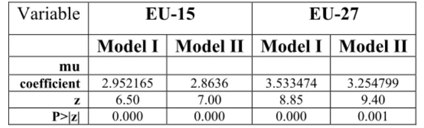
The high values of the mean, µ, of the first part of the cost function’s error, capturing the

effects of the inefficiency, as defined above, indicates that in all circumstances (see Table 1,

below, with values taken from Appendix IV), technical inefficiencies exist and they are

always statistically important. This means that the use of a traditional cost function with no

technical inefficiency effects would not be an adequate representation of the data.

A more careful observation of the values provided in Table 1 allows us to conclude that

(12)

possible difficulties of the EU banking institutions in the process of adaptation to the new

conditions of the enlarged market.

TABLE 1 – Summary of the obtained results for the mean, µ

Variable EU-15 EU-27

Model I Model II Model I Model II

mu

coefficient 2.952165 2.8636 3.533474 3.254799

z 6.50 7.00 8.85 9.40

P>|z| 0.000 0.000 0.000 0.001

The presence of inefficiency is also confirmed by the high values of the contribution of the

inefficiency (u) to the total error. The obtained values of the ₂ ₂

2

v u

u

σ σ

σ γ

+

= , reported in Table

2, reveal that in all panels the inefficient error term amounts to around 98%. This implies that

the variation of the total cost among the different EU countries was almost solely due to the

differences in their cost inefficiencies.

TABLE 2 – Summary of the obtained results for the contribution of the inefficient

error term to total variance, γ

gamma

Coefficient .9743051 .9769977 .9803236 .9796408 Standard error .0118859 0.0102856 .0057757 .0059013

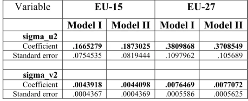
The previous results are confirmed by the comparison of the values of the variances of the

inefficient error term (σu) and the random disturbances (σv), which are presented in Table 3.

1

(13)

In all situations, the variance is mostly due to the inefficient term and the EU-15 panel is

revealed to be much more homogeneous than the EU-27 panel.

TABLE 3 – Summary of the obtained results for the variance of the inefficient error term (σu) and the noise (σv)

sigma_u2

Coefficient .1665279 .1873025 .3809868 .3708549

Standard error .0754535 .0819444 .1097962 .105689

sigma_v2

Coefficient .0043918 .0044098 .0076469 .0077072

Standard error .0004367 .0004369 .0005586 .0005625

According to the estimation results of the cost function, also displayed in Appendix IV, we

can see that in all situations, the total cost (more precisely, the sum of interest expenses plus

the operating expenses) increases mostly with the price of the borrowed funds (W1, here

represented by the ratio interest expenses over the sum of the deposits). However, the contrary

appears likely to have occurred with the other two inputs: the price of capital (W2, with the

proxy ratio of the non-interest expenses over fixed assets) and the price of labour (W3, the

ratio personnel expenses over the number of employees). This may be due either to the chosen

proxies or to the decreasing importance of the traditional production factors in bank activities.

On the other hand, as expected, the total cost always increases with the provided securities

(Y2) and the other earning assets (Y3, here the difference between the earning assets and the

total loans). As for the other output, total loans (Y1), they clearly also increase the total cost,

but only in the EU-27 panel.

With regard to the other explanatory variables, the results are statistically significant only for

(14)

thereby confirming our expectations: total cost clearly increases with the equity ratio and

decreases with the revenue over expenses ratio.

From the residuals of the estimated cost frontier functions (Model I of Appendix IV), we also

obtain the country efficiency scores, which are presented in Appendix V. For each panel, the

100% result is obtained by the country with the best practice, that is, the country with least

waste in its production process. All the other countries are classified in relation to each

panel´s benchmark.

Again according to the results reported in Appendix V, we see that the inclusion of the new

EU member-states produces a very small decrease in the mean score and the median of cost

efficiency and slightly increases the standard deviation. Regarding the country efficiency

scores, the results for the EU-27 panel clearly show that the all of the 12 “new” member-states

are situated below the mean efficiency. However, there are also three “old” members

(specifically, Austria, Portugal and Greece) which not only have the worst scores in the

EU-15 panel, but also occupy low positions in the EU-27 ranking, indeed obtaining worse results

than some of the “new” member-states.

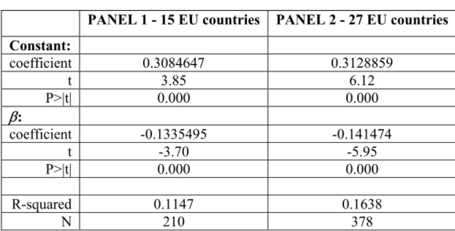
In order to test the degrees of convergence within the two panels of countries, we use the

predicted values of efficiency obtained with the estimated cost model (Model II of Appendix

IV) to estimate the previously-presented beta-convergence model (see equation [2]).

Borrowing from economic growth theory, we know that a negative value of the estimated

betas reveals convergence and that the higher is beta, the faster will the convergence process

be.

The results obtained with our model are reported in Table 4 (we have omitted the results for

(15)

Table 4 – β-Convergence estimates

PANEL 1 - 15 EU countries PANEL 2 - 27 EU countries Constant:

coefficient 0.3084647 0.3128859

t 3.85 6.12

P>|t| 0.000 0.000

β:

coefficient -0.1335495 -0.141474

t -3.70 -5.95

P>|t| 0.000 0.000

R-squared 0.1147 0.1638

N 210 378

From the results reported in Table 4, we can conclude that there is a convergence process

across EU countries in both panels, since the values of the estimated betas are statistically

significant and negative but they are relatively small, revealing that this convergence is not a

very fast process.

Appendix VI presents the results obtained with the input-oriented Data Envelopment Analysis

(DEA) which, as was mentioned earlier, does not require the specification of a functional

form. In our estimations, we use the same three inputs (borrowed funds, physical capital and

labour, as defined previously) and the same three outputs (total loans, total securities and

other earning assets). In this case, a perfectly efficient country will be situated on the efficient

frontier, which is defined, for each panel, with the combinations of the best-practice

observations of the panel. In addition, the relative measure of any country´s inefficiency will

be its distance from the efficient frontier.

As expected, the DEA efficiency scores are lower than those obtained with the estimation of

the Stochastic Cost Frontier (SCF), since DEA does not allow for the decomposition between

“pure” technical inefficiency and “noise”. Now there is a clearer decrease of the average

(16)

median also declines from 78% to 75%, while the standard deviation increases from 16.2% to

22.7%.

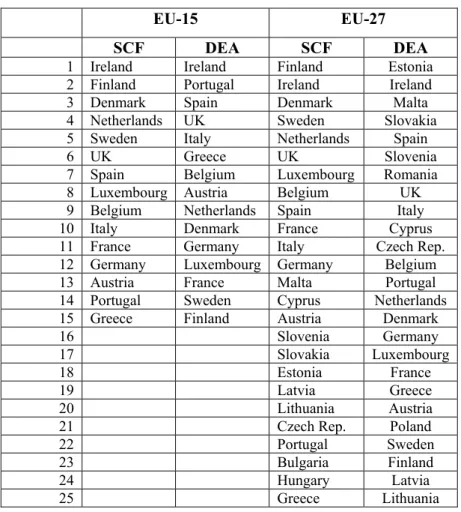
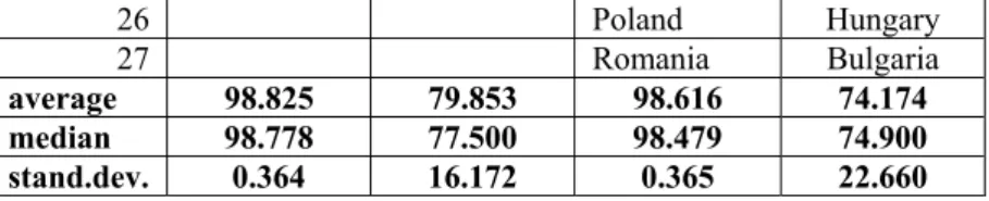
Table 5 below allows the comparison between the country efficiency rankings which were

obtained with both the estimated SCF and DEA estimations. In spite of the methodological

differences, there are only few remarkable changes in the countries’ ranking positions. For

instance, Finland is very well classified with the SCF, but falls dramatically with the DEA

estimations. However, it is worth noting that according to the data presented in Appendix III,

the Finnish banks represent, on average, only around 0.5% of all considered banks. Generally

speaking, Table 5 shows that for some of the more representative countries, even when the

ranking position is not exactly the same, a good score with the SCF is almost always

confirmed with a similarly good position with DEA (and vice versa).

Table 5 – SCF and DEA country efficiency rankings

EU-15 EU-27

SCF DEA SCF DEA 1 Ireland Ireland Finland Estonia 2 Finland Portugal Ireland Ireland 3 Denmark Spain Denmark Malta 4 Netherlands UK Sweden Slovakia 5 Sweden Italy Netherlands Spain

6 UK Greece UK Slovenia

7 Spain Belgium Luxembourg Romania 8 Luxembourg Austria Belgium UK 9 Belgium Netherlands Spain Italy 10 Italy Denmark France Cyprus 11 France Germany Italy Czech Rep. 12 Germany Luxembourg Germany Belgium 13 Austria France Malta Portugal 14 Portugal Sweden Cyprus Netherlands 15 Greece Finland Austria Denmark

16 Slovenia Germany

17 Slovakia Luxembourg

18 Estonia France

19 Latvia Greece

20 Lithuania Austria

21 Czech Rep. Poland

22 Portugal Sweden

23 Bulgaria Finland

24 Hungary Latvia

(17)

26 Poland Hungary

27 Romania Bulgaria

average 98.825 79.853 98.616 74.174 median 98.778 77.500 98.479 74.900

stand.dev. 0.364 16.172 0.365 22.660

Finally, in order to test the differences in the efficiency results in two specific periods that

coincide both with the implementation of the EMU and with the last EU enlargement, we

apply the DEA estimates for the two panels of countries (EU-15 and EU-27) during two time

sub-periods: 2000-2008 and 2004-2008. The average results2 are presented below in Table 6,

where we also include the average results for the entire time period (1994-2008). These

results allow us to conclude that the EU enlargement not only increased heterogeneity (the

standard deviations are always greater in the EU-27 panels), but also contributed to the

decrease of the average and the median of the efficiency scores.

Furthermore, and again according to the results reported in Table 6, for both panels (EU-15

and EU-27), there has been an increase in efficiency since the implementation of the EMU

(the results for the time period 2000-2008 are always higher than those for the entire period,

1994-2008). However, efficiency decreased slightly after the most recent EU enlargement

process (the results for the period 2004-2008 are inferior to those obtained for 2000-2008).

Table 6 –DEA average efficiency by panels and time periods

1994-2008 2000-2008 2004-2008 EU-15 EU-27 EU-15 EU-27 EU-15 EU-27

Average 79.853 74.174 82.953 81.033 82.013 80.589

Median 77.500 74.900 82.600 82.400 82.200 83.300

stand.dev. 16.172 22.660 17.109 16.262 17.039 18.458

2

(18)

5. Discussion and conclusions

The two approaches to efficiency measurement, SFA and DEA, rely on the concept of

efficiency that relates, in a production function, the allocation of scarce resources or inputs to

the obtained results or outputs defining the production possibility frontier. Thus, with both

approaches, technical efficiency is always a relative measure of the distance to the frontier

and depends on the specific inputs and outputs and the definition of the production function.

The SFA approach is a parametric method that requires the econometric estimation of the

(cost or profit) function. One of its main advantages is to allow the decomposition of the

deviations from the efficient frontier between the stochastic error and pure inefficiency.

Another important advantage of this approach is the guarantee that if we include an irrelevant

variable in the function, the method will detect this irrelevance and the variable will have a

very low or even zero weight in the definition of the efficiency results.

On the other hand, the DEA approach may be more flexible, as it does not require the

estimation of any econometric function. One of its main advantages is to provide efficiency

scores even in the presence of relatively few observations, since for each situation, DEA will

take the available data to define the efficiency frontier with the combinations of the

best-practice observations. All production units are situated either on or below the defined

efficiency frontier and the efficiency measure is simply the distance of each production unit to

the frontier.

So, the natures of these two approaches are very different and even when they are estimating

the underlying efficiency values of the same production units, using the same inputs to

produce the same outputs, SFA and DEA can provide different efficiency scores for some or

even all the units under analysis. As each method has its own advantages, neither of them

provides results that can be considered, for all data sets, much better than the results obtained

(19)

In this paper, we chose to use both the SFA and DEA approaches and, when possible, we

compare their results. Following the intermediation approach, we take into account the

available data and the specific character of the bank production activities and consider three

inputs (total loans, total securities and other earning assets) and the prices of three outputs

(borrowed funds, physical capital and labour). For the application of the SFA, we opt to

estimate stochastic cost frontier (SCF) functions and suppose that the total cost depends on

three other explanatory variables: the number of banks, the equity ratio and the ratio revenue

over expenses.

We took our data from the Bankscope database, which is universally recognised as one of the

most appropriate banking data sources as it guarantees standardisation and comparability and

provides data on banks accounting for 90% of total bank assets. Nevertheless, in spite of its

recognised advantages, Bankscope data can still be very unbalanced, at least insofar as the

number of included banks is concerned. In this paper, we use the available data from the

consolidated accounts of the commercial and savings banks of all EU countries for the time

period 1994-2008. Approximately 30% of the included banks are from one country

(Germany), while the banks of four countries (Germany, France, Italy and UK) account for

half of all the banks considered (see Appendix III). The main argument is that this reflects the

reality of European banking, with the dominant power of the rich, large countries. On the

other hand, even when we recognise that the number of banks can be important, we should

also take into account their weight and the degree of concentration in the specific bank

market.

Another important issue concerns the variables used. As Bankscope does not directly provide

the prices of the production inputs, we consider proxies of these prices. For the price of the

borrowed funds, we took the ratio interest expense over the sum of deposits; for physical

(20)

ratio personnel expenses over the number of employees. This may be one of the explanations

for the unexpected signals that we obtained for the influence of the labour and capital in the

total cost in the estimated cost frontier functions. Another possible reason stems from the

specificity of the banking production process, which actually depends much more on the

borrowed funds that on the traditional production factors.

The estimated SCF function also confirms that the total cost depends on the chosen outputs. It

mostly increases with the provided securities and the other earning assets, as well as with the

total loans, although less clearly. As for the other explanatory variables included in the cost

function, the results confirm that total cost clearly increases with the equity ratio and

decreases with the ratio revenue over expenses.

Furthermore, the results obtained with the SCF function confirm the existence of statistically

important technical inefficiencies and that these inefficiencies increase with the inclusion of

the new EU member-states, since all of the countries have had to adapt to the new competitive

conditions of the enlarged market.

These results are also confirmed by the DEA approach, which clearly shows that efficiency

decreased with the inclusion of the new EU member-states. Furthermore, the DEA results

allow us to analyse the evolution of the efficiency scores after the implementation of EMU

(2000-2008) and in the years after the recent EU enlargement (2004-2008). Concentrating on

the average levels of efficiency, we may conclude that while the implementation of the EMU

has contributed to an increase of bank efficiency, the contrary appears to have happened more

recently with the enlargement process. In line with these conclusions, the country ranking

positions obtained with SCF estimates clearly show that most of the new member-states are

situated below the average efficiency scores, together with some “old” EU members which

(21)

Moreover, the comparison of the results obtained with SCF and DEA country efficiency

rankings allows us to conclude that, in spite of the different methodologies, and with few

exceptions, countries that are well-classified with one approach are also in a good position

with the other approach, and vice versa.

Thus, even if it is true that European integration may contribute to the increase of the average

efficiency scores, some EU members are still facing difficulties to catch up with the levels of

the best performers. Nevertheless, our convergence estimates confirm that there is a clear

convergence process among EU members, although the pace continues to be very slow, with

no guarantee that full integration will be achieved in the near future.

References

Affinito, M. and Farabullini, F. (2009) “Does the Law of One Price hold in Euro-Area Retail Banking? An Empirical Analysis of Interest Rate Differentials across the Monetary Union” International Journal of Central Banking, 5, pp. 5-37.

Aigner, D.J., Lovell C.A.K. and Schmidt, P. (1977) “Formulation and estimation of stochastic frontier production function models”, Journal of Econometrics, 6, pp. 21-37.

Altunbas, Y., Gardener, E.P.M., Molyneux, P. and Moore, B. (2001) “Efficiency in European banking” European Economic Review, 45, pp. 1931-1955.

Altunbas, Y. and Marquês, D. (2007) “Mergers and acquisitions and bank performance in Europe. The role of strategic similarities”, Journal of Economics and Business, 60, pp. 204-222.

Banker, R. D., Charnes, A. and Cooper, W. W. (1984) “Some models for the estimating technical and scale inefficiency in Data Envelopment Analysis”, Management Science, 30, pp. 1078-1092.

Barros, C., Ferreira, C. and Williams, J. (2007) “Analysing the determinants of performance of best and worse European banks: A mixed logit approach”, Journal of Banking and Finance, 31, pp. 2189-2203.

Battese, G. E. and Coelli, T. (1988) “Prediction of firm-level technical efficiencies with a generalized frontier production function and panel data”, Journal of Econometrics, 38, pp. 387-399.

Battese, G. E. and Coelli, T. (1992) “Frontier Production Functions, Technical Efficiency and Panel Data: With Application to Paddy Farmers in India”, Journal of Productivity Analysis, 3, pp. 153-169.

Battese, G. E. and Coelli, T. (1995) “A Model for Technical Inefficiency Effects in a Stochastic Frontier Production Function for Panel data”, Empirical Economics, 20, pp. 325-332.

Beck, T., Demirguç-Kunt, A. and Levine, R. (2003a) “Law, endowments, and finance”, Journal of Financial Economics, 70, 137–181.

Beck, T., Demirguç-Kunt, A. and Levine, R. (2003b) “Law and finance. Why does legal origin matter?” Journal of Comparative Economics, 31, 653–675.

Beck, T., Levine, R. (2004) “Stock markets, banks and growth: Panel evidence”, Journal of Banking and Finance, 28, 423–442.

(22)

Berger, A. N. (2007) “International Comparisons of Banking Efficiency”, Financial Markets, Institutions and Instruments, 16, pp. 119-144.

Berger, A.N. and Humphrey, D. B. (1991) “The dominance of inefficiencies over scale and product mix economies in banking”, Journal of Monetary Economics, 28, pp. 117-148.

Berger, A.N. and Mester, L. J. (1997) “Inside the black box: What explains differences in inefficiencies of financial institutions?”, Journal of Banking and Finance, 21, pp. 895-947.

Berger, A.N., DeYoung, R. and Udell, G.F. (2001) “Efficiency barriers to the consolidation of the European Financial services industry” European Financial Management, 7, pp. 117-130.

Bikker, J.A., Spierdijk, J. and Finnie, P. (2006) The impact of bank size on market power, DNB Working Paper No. 120.

Bonin, J.P., Hasan, I. and Wachtel, P. (2005) “Bank performance, efficiency and ownership in transition countries” Journal of Banking and Finance, 29, pp. 31-53.

Bos, J. W. B. and Kool, C. J. M. (2006) “Bank efficiency: The role of bank strategy and local market conditions” Journal of Banking and Finance, 30, pp. 1953-1974.

Bos, J. W. B. and Schmiedel, H. (2007) “Is there a single frontier in a single European banking market?” Journal of Banking and Finance, 31, pp. 2081-2102.

Cabral I., Dierick, F. and Vesala, J. (2002) Banking Integration in the Euro Area, ECB Occasional Paper Series No. 6. .

Campa, J.M. and Hernando, I. (2006) “M&As performance in the European financial industry”,

Journal of Banking and Finance, 28, pp. 2077-2102.

Cappiello, L., Hodahl,P., Kadareja, A. and Manganelli, S. (2006) The impact of the euro on financial markets, ECB Working Paper Series No. 598.

Casu, B., Girardone, C. and Molyneux, P. (2004) “Productivity change in European banking: A comparision of parametric and non-parametric approaches, Journal of Banking and Finance, 28, pp. 2521-2540.

Casu, B. and Girardone, C. (2009) “Competition issues in European banking” Journal of Financial Regulation and Compliance, 17, pp. 119-133.

Casu, B. and Girardone, C. (2010) “Integration and efficiency convergence in EU banking markets”,

Omega, 38, pp. 260-267.

Charnes A., Cooper W.W. and Rhodes, E. (1978) “Measuring the Efficiency of Decision-Making Units”, European Journal of Operational Research, 2, pp. 429 - 444.

Coelli, T., D., Rao, S. P. and Battese, G. E. (1998) An introduction to efficiency and productivity analysis, Kluwer Academic Publishers, Boston.

Cook W.D., Seiford L.M. (2009) “Data envelopment analysis (DEA) - Thirty years on”, European Journal of Operational Research, 192, pp. 1-17.

Dermine, J. (2006) “European banking integration: Don’t put the cart before the horse”, Financial Markets, Institutions and Instruments, 15, pp. 57-106. .

Diaz, B. D., Olalla, M. G and Azofra, S. S. (2004) “Bank acquisitions and performance: evidence from a panel of European credit entities” Journal of Economics and Business, 56, pp. 377-404.

European Central Bank (2007) Financial integration in Europe.

European Central Bank (2008) Financial integration in Europe.

Farrell, M.J. (1957) “The Measurement of Productive Efficiency” Journal of the Royal Statistical Society, 120, pp. 253-290.

Frerier, G.D. and Lowell, C.A.K. (1990)” Measuring cost efficiency in banking: Econometric and linear programming evidence”, Journal of Econometrics46, pp. 229-245.

Gardener, E.P.M., Molyneux, P. and Moore, B. (ed.) (2002) - Banking in the New Europe – The Impact of the Single Market Program and EMU on the European Banking Sector, Palgrave, Macmillan.

Goddard, J.A., Molyneux, P. and Wilson, J. O. S. (2001) European banking efficiency, technology and growth, John Willey and Sons.

Goddard, J.A., Molyneux, P. and Wilson, J. O. S. (2007) “European banking: an overview”,

Journal of Banking and Finance, 31, pp. 1911-1935. Greene, W.M. (1990) “A gamma-distributed stochastic frontier model”, Journal of Econometrics, 46, pp. 141-163.

(23)

Greene, W.H. (2003) Econometric Analysis, 5th edn., Upper Saddle River, NJ: Prentice

Gropp, R. and Kashyap, A. K. (2009) “A New Metric for Banking Integration in Europe”, NBER Working Paper No. 14735.

Guiso, L., Jappelli, T., Padula, M. and Pagano, M. (2004) “Financial market integration and economic growth in the EU”, Economic Policy, 40, pp. 523-577.

Hartmann P., Maddaloni, A. and Manganelli, S. (2003) “The euro area financial system: structure integration and policy initiatives” Oxford Review of Economic Policy, 19, pp. 180-213.

Holló, D. and Nagy, M. (2006) “Bank Efficiency in the enlarged European Union” in The banking

system in emerging economies: how much progress has been made?, BIS Papers, N. 28, Bank of

International Settlements Papers, Monetary and Economic Department, pp. 217-235.

Hughes, J. P. and Mester, L. (2008) Efficiency in banking: theory, practice and evidence, Federal Reserve Bank of Philadelphia, Working Paper 08-1. Hall

Jondrow, J., Lovell, C.A.K., Materov, I.S. and Schmidt, P. (1982) “On estimation of technical inefficiency in the stochastic frontier production function model”, Journal of Econometrics, 19, pp. 233-238

Kasman, A. and Yildirim, C. (2006) “Cost and profit efficiencies in transition banking: the case of new EU members”, Applied Economics, 38 pp. 1079-1090. .

Kumbhakar, S.C. and Lovell, C.A.K. (2000) Stochastic Frontier Analysis, Cambridge University Press, Cambridge.

Kumbhakar, S.C., Lozano-Vivas, A., Lovell, C.A.K. and Hasan, I. (2001) “The effects of deregulation on the performance of financial institutions: The case of Spanish savings banks”, Journal of Money, Credit and Banking, 33, pp. 101-120.

Lensink, R., Meesters, A. and Naaborg, I. (2008) “Bank efficiency and foreign ownership: Do good institutions matter” Journal of Banking and Finance, 32, pp. 834-844.

Manna, M. (2004) Developing statistical indicators of the integration of the euro area banking system, ECB Working Paper Series No.300. .

Meeusen, W. and Van den Broeck, J. (1977) “Efficiency estimation from a Cobb-Douglas production function with composed error” International Economic Review, 18, pp. 435-444.

Molyneux, P. (2003) “Does size matter?” Financial restructuring under EMU, United Nations Universiy, Institute for New Technologies, Working Paper No. 03-30.

Murinde, V., Agung, J. and Mullineux, A. W. (2004) “patterns of corporate financing and financial system convergence in Europe”, Review of International Economics, 12, pp. 693-705.

Resti, A. (1997) “Evaluating the cost-efficiency of the Italian banking system: what can be learn from the joint application of parametric and non-parametric techniques, Journal of Banking and Finance, 21, pp. 221-250.

Rossi, S., M. Schwaiger and G. Winkler (2005) Managerial Behaviour and Cost/Profit Efficiency in the Banking Sectors of Central and Eastern European Countries, Working Paper 96, Oesterreichische Nationalbank.

Schaeck, K. and Cihak, M. (2007) Bank competition and capital ratio, IMF Working Paper

WP/07/216.

Schure, P., Wagenvoort, R. and O’Brien, D. (2004) “The efficiency and the conduct of European banks: Developments after 1992” Review of Financial Economics, 13, pp.371–396.

Sealey, C., and Lindley, J. T. (1977) “Inputs, outputs and a theory of production and cost at depository financial institution” Journal of Finance, 32, pp. 1251–1266.

Stevenson, R. F. (1980) “Likelihood Functions for Generalized Stochastic Frontier Estimation”,

Journal of Econometrics, 13, pp. 57-66.

Sturm, J-E and Williams, B. (2010) “What determines differences in foreign bank efficiency?

Australian evidence”, Journal of International Financial markets, Institutions and Money, 20, pp.

284-309.

Thanassoulis, E., Portela, M. C. S. and Despic, O. (2008) “DEA – The mathematical programming

approach to efficiency analysis” in Fried, H. O., Lovell, C. A. and Schmidt, K. S. S. (eds.), The

measurement of productive efficiency and productivity growth, Oxford University Press.

Tortosa-Ausina, E. (2002) “Exploring efficiency differences over time in the Spanish banking

(24)

Vives, X. (2001) – “Restructuring Financial Regulation in the European Monetary Union”, Journal of Financial Services Research, 19, pp. 57-82.

Weill L. (2004), Measuring Cost Efficiency in European Banking: A comparison of frontier techniques, Journal of Productivity Analysis, 21, 133-152.

Weill, L. (2009) “Convergence in banking efficiency across European countries”, Journal of International Financial Markets Institutions and Money, 19, pp. 818-833.

Williams, J. and Nguyen, N. (2005) “Financial liberalisation, crisis and restructuring: A comparative

study of bank performance and bank governance in South East Asia”, Journal of Banking and Finance,

29, pp. 2119-2154.

Wheelock, D.C. and Wilson, P. W. (1999) “Technical progress, inefficiency and productivity change in US banking: 1984-1993” Journal of Money, Credit and Banking, 31, pp. 213-234.

APPENDIX I – Panel stochastic frontier models

For panel data models, and particularly with stochastic frontier models, it is necessary not only to suppose the normality for the noise error term (v) and half- or truncated normality for the inefficiency error term (u), but also to assume that the firm-specific level of inefficiency is uncorrelated with the input levels. This type of model also addresses the fundamental question of whether and how inefficiencies vary over time.

Following Battese and Coelli (2008) and Battese et al. (1989), a general panel stochastic frontier model, with Ti time observations of i units, can be represented as:

[

]

[ ]

2 2 , 0 ~ , ~ v it u i i it it it T it N v N u u v x Y σ σ µ β

α + + −

=

Using the Greene (2003) reparameterisation and the truncated normal distribution of ui, we have:

[

]

(

)( )

2 2 * 2 2 * , 2 , 1 , 1 1 1 * * * * * * ,..., , u i i v u i i it T it it i i i i i i i i i i T i i i i T x y u E i

σ

γ

σ

λ

γ

αβ

ε

γ

µ

γ

µ

σ

µ

σ

µ

φ

σ

µ

ε

= = + = − = − − + =                  − Φ       + =

(25)

APPENDIX II – Data Envelopment Analysis (DEA)

DEA was originally presented in the paper of Charles et al. (1978), assuming constant returns to scale, which can be accepted as optimal but only in the long run. Later, Banker et al. (1984) introduced an additional convexity constraint (λ) and allowed for variable returns to scale.

Following Banker et al. (1984), we can assume that at any time t, there are N decision-making units (DMUs) that use a set of X inputs (X = x1, x2, ..., xk) to produce a set of Y

outputs (Y = y1, y2, ..., ym), thus obtaining the DEA input-oriented efficiency measure of

every i DMU, solving the following optimisation problem:

∑

= = = = ≥ ≤ ≥ N 1 r N 1 r t kr N 1 r t mr , 1 0 x y . . min t r t r t ki i t r t mi t r i x y t s λ λ θ λ λ θ λ θ

APPENDIX III – Number of banks (and %) by country

Country 1994 2000 2008 Average

(1994-2008)

Austria 54 (2.34) 129 (4.92) 147 (6.92) 127 (4.90)

Belgium 88 (3.82) 68 (2.60) 34 (1.60) 72 (2.78)

Bulgaria 10 (0.43) 25 (0.95) 21 (0.99) 23 (0.89)

Cyprus 12 (0.52) 23 (0.88) 9 (0.42) 18 (0.69)

Czech Rep. 24 (1.04) 27 (1.03) 20 (0.94) 26 (1.00)

Denmark 98 (4.25) 123 (4.69) 109 (5.13) 116 (4.48)

Estonia 9 (0.39) 10 (0.38) 10 (0.47) 11 (0.42)

Finland 11 (0.48) 14 (0.53) 12 (0.56) 13 (0.50)

France 350 (15.18) 308 (11.76) 204 (9.60) 297 (11.46)

Germany 786 (34.08) 771 (29.43) 593 (27.92) 738 (28.48)

Greece 25 (1.08) 26 (0.99) 29 (1.37) 32 (1.24)

Hungary 30 (1.30) 39 (1.49) 26 (1.22) 34 (1.31)

Ireland 24 (1.04) 42 (1.60) 40 (1.88) 42 (1.62)

Italy 177 (7.68) 216 (8 .24) 199 (9.37) 231 (8.92)

Latvia 16 (0.69) 25 (0.95) 33 (1.55) 27 (1.04)

Lithuania 7 (0.30) 16 (0.61) 15 (0.71) 14 (0.54)

Luxembourg 118 (5.12) 112 (4.27) 80 (3.77) 106 (4.09)

Malta 8 (0.35) 10 (0.38) 14 (0.66) 12 (0.46)

Netherlands 50 (2.17) 50 (1.91) 41 (1.93) 57 (2.20)

Poland 33 (1.43) 50 (1.91) 37 (1.74) 48 (1.85)

Portugal 34 (1.47) 37 (1.41) 25 (1.18) 36 (1.39)

Romania 3 (0.13) 31 (1.18) 27 (1.27) 23 (0.89)

Slovakia 11 (0.48) 22 (0.84) 16 (0.75) 19 (0.73)

Slovenia 14 (0.61) 25 (0.95) 21 (0.99) 23 (0.89)

Spain 172 (7.46) 204 (7.79) 136 (6.40) 196 (7.56)

Sweden 14 (0.61) 22 (0.84) 78 (3.67) 60 (2.32)

UK 128 (5.55) 195 (7.44) 148 (6.97) 190 (7.33)

(26)

APPENDIX IV – Estimates with Cost Frontier Function

PANEL 1 - 15 EU countries

(1994 – 2008)

PANEL 2 - 27 EU countries

(1994 – 2008)

Variable Model I Model II Variable Model I Model II

W1: W1:

coefficient .7978371 .7182306 coefficient .8743844 .8159698

z 5.99 6.59 z 8.33 8.72

P>|z| 0.000 0.000 P>|z| 0.000 0.000

W2: W2:

coefficient -.4135728 -.3531588 coefficient -6.864385 -.7367332

z -3.45 -4.08 z -6.18 -7.13

P>|z| 0.001 0.000 P>|z| 0.000 0.000

W3: W3:

coefficient -.1162695 -.0858007 coefficient -.1191528 -.1065062

z -2.43 -2.00 z -3.33 -3.46

P>|z| 0.015 0.045 P>|z| 0.001 0.001

Y1: Y1:

coefficient -.1072872 coefficient .3433489 .3308214

z -0.89 z 5.65 10.66

P>|z| 0.376 P>|z| 0.000 0.000

Y2: Y2:

coefficient .1749893 coefficient .103594

z 0.81 z 1.42

P>|z| 0.418 P>|z| 0.157

Y3: Y3:

z 3.03 30.54 z 3.24 17.01

P>|z| 0.002 0.000 P>|z| 0.001 0.000

P1: P1:

z -5.15 -25.26 z -2.39 -5.66

P>|z| 0.000 0.000 P>|z| 0.017 0.000

P2: P2:

z 1.21 2.48 z 2.71 5.77

P>|z| 0.228 0.013 P>|z| 0.007 0.000

P3: P3:

coefficient .1058051 .1342023 coefficient -0.304238

z 1.25 7.23 z -1.06

P>|z| 0.212 0.000 P>|z| 0.288

P4: P4:

coefficient .0753658 .09093 coefficient .000928

z 2.21 3.76 z 0.05

P>|z| 0.027 0.000 P>|z| .964

P5: P5:

z -2.25 -3.05 z -3.73 -5.03

P>|z| 0.025 0.002 P>|z| 0.000 0.000

P6: P6:

coefficient .0505409 coefficient .1639128 .1834019

z 0.74 z 3.96 6.12

P>|z| 0.461 P>|z| 0.000 0.000

P7: P7:

coefficient -.0054226 coefficient -.011956 -.0106709

z -0.80 z -2.24 -2.06

P>|z| 0.461 P>|z| 0.025 0.040

P8: P8:

coefficient -.0342686 -.0344847 coefficient -.005493

z -2.82 -2.95 z -0.68

P>|z| 0.005 0.003 P>|z| 0.495

P9: P9:

(27)

z 3.10 3.02 z 2.21 3.06 P>|z| 0.002 0.002 P>|z| 0.027 0.002

Z1: O1:

coefficient -.0316589 -.0329478 coefficient -.0006337

z -1.61 -1.80 z -0.03

P>|z| 0.107 0.071 P>|z| 0.974

Z2: O2:

z 4.78 5.77 z 3.77 3.64

P>|z| 0.000 0.000 P>|z| 0.000 0.000

Z3: O3:

coefficient -1.010373 -.9939596 coefficient -.7982632 -.7986451

z -8.27 -8.19 z -12.15 -12.17

P>|z| 0.000 0.000 P>|z| 0.000 0.000

mu mu

coefficient 2.952165 2.8636 coefficient 3.533474 3.254799 z 6.50 7.00 z 8.85 9.40 P>|z| 0.000 0.000 P>|z| 0.000 0.001

lnsigma2 lnsigma2

coefficient -1.766562 -1.65176 coefficient -.945118 -.9713751 z -4.00 -3.87 z -3.35 -3.48 P>|z| 0.000 0.000 P>|z| 0.001 0.001

ilgtgamma ilgtgamma

Coefficient 3.635433 3.748892 Coefficient 3.908464 3.873654 z 7.66 8.19 z 13.05 13.09 P>|z| 0.000 0.000 P>|z| 0.000 0.000

sigma2 sigma2

Coefficient .1709196 .1917123 Coefficient .3886337 .3785621

Standard error .0754052 .0819039 Standard error .1097808 .1056769

gamma gamma

Coefficient .9743051 .9769977 Coefficient .9803236 .9796408

Standard error .0118859 0.0102856 Standard error .0057757 .0059013

sigma_u2 sigma_u2

sigma_v2 sigma_v2

Wald chi2 6653.75 6642.71 Wald chi2 13032.10 12927.96 Prob > chi2 0.0000 0.0000 Prob > chi2 0.0000 0.0000

Log likelihood 243.80243 242.49131 Log likelihood 322.8634 321.74196

N 225 225 N 405 405

(*) TC = Total cost (dependent variable)= natural logarithm of the sum of the interest expenses plus the total operating expenses

Inputs:W1 = Price of the borrowed funds = natural logarithm of the ratio interest expenses over the sum of deposits;

W2 = Price of physical capital = natural logarithm of the ratio noninterest expenses over fixed assets

W3 = Price of labour = natural logarithm of the ratio personnel expenses over the number of employees

Outputs: Y1 = Total loans = natural logarithm of the loans

Y2 = Total securities = natural logarithm of the total securities

Y3 = Other earning assets= natural logarithm of the difference between the total earning assets and the

(28)

Products of Inputs and Outputs: P1 = W1 * Y1; P2 = W1 * Y2; P3 = W1 * Y2; P4 = W2 * Y1; P5 = W2 * Y2; P6 =

W2*Y3; P7 = W3 * Y1; P8 = W3 * Y2; P9 = W3 * Y3

Other variables:Z1 = Number of companies = natural logarithm of the number of companies included

Z2 = Equity ratio = natural logarithm of the ratio equity over total assets

Z3 = Ratio revenue over expenses = natural logarithm of the ratio of the total revenue over

the total expenses

APPENDIX V – Cost efficiency rankings obtained from SCF estimations

EU-15 (1994-2008)

EU-27 (1994-2008) Country Efficiency

Ranking

Country Efficiency Ranking 1 Ireland 100.000 Finland 100.000 2 Finland 98.990 Ireland 98.987

3 Denmark 98.952 Denmark 98.971 4 Netherlands 98.874 Sweden 98.905

5 Sweden 98.867 Netherlands 98.869

6 UK 98.801 UK 98.785

7 Spain 98.786 Luxembourg 98.784 8 Luxembourg 98.778 Belgium 98.777 9 Belgium 98.768 Spain 98.760 10 Italy 98.736 France 98.733 11 France 98.712 Italy 98.729

12 Germany 98.678 Germany 98.720 13 Austria 98.573 Malta 98.559

14 Portugal 98.445 Cyprus 98.479 15 Greece 98.409 Austria 98.474

16 Slovenia 98.446

17 Slovakia 98.411

18 Estonia 98.402

19 Latvia 98.394

20 Lithuania 98.378

21 Czech Rep. 98.348

22 Portugal 98.331

23 Bulgaria 98.329

24 Hungary 98.286

25 Greece 98.284

26 Poland 98.274

27 Romania 98.211

average 98.825 98.616

median 98.778 98.479

(29)

Appendix VI – Estimates with input-oriented Data Envelopment Analysis (DEA): EU-15 and EU-27 for the time period 1994-2008

EU-15

(1994-2008)

EU-27

(1994-2008)

Country Efficiency Ranking

Country Efficiency Ranking

1 Ireland 100.00 Estonia 100.00 2 Portugal 100.00 Ireland 100.00

3 Spain 100.00 Malta 100.00

4 UK 100.00 Slovakia 100.00

5 Italy 95.80 Spain 100.00

6 Greece 84.40 Slovenia 97.60

7 Belgium 81.60 Romania 97.40

8 Austria 77.50 UK 96.40

9 Netherlands 75.50 Italy 95.80

10 Denmark 73.70 Cyprus 88.70

11 Germany 70.50 Czech Rep. 87.40 12 Luxembourg 68.80 Belgium 81.50 13 France 66.20 Portugal 76.40 14 Sweden 52.00 Netherlands 74.90 15 Finland 51.80 Denmark 73.50

16 Germany 70.40

17 Luxembourg 68.20

18 France 66.20

19 Greece 64.20

20 Austria 63.80

21 Poland 58.70

22 Sweden 52.00

23 Finland 49.30

24 Latvia 43.00

25 Lithuania 40.30

26 Hungary 34.50

27 Bulgaria 22.50