Maximum a posteriori joint state path and parameter estimation in stochastic differential equations

(1)

Universidade Federal de Minas Gerais

Programa de Pós-Graduação em Engenharia Elétrica

Maximum

a Posteriori

Joint State Path

and Parameter Estimation in

Stochastic Diﬀerential Equations

(2)

(3)

(4)

(5)

(6)

(7)

Having all the answers just means you’ve been asking boring questions.

Emily Horn and Joey Comeau

(8)

(9)

Abstract

A wide variety of phenomena of engineering and scientific interest are of a continuous-time nature and can be modeled by stochastic differential equations (SDEs), which represent the evolution of the uncertainty in the states of a system. For systems of this class, some parameters of the SDE might be unknown and the measured data often includes noise, so state and parameter estimators are needed to perform inference and further analysis using the system state path. One such application is the flight testing of aircraft, in which flight path reconstruction or some other data smoothing technique is used before proceeding to the aerodynamic analysis or system identification.

The distributions of SDEs which are nonlinear or subject to non-Gaussian measurement noise do not admit tractable analytic expressions, so state and parameter estimators for these systems are often approximations based on heuristics, such as the extended and unscented Kalman smoothers, or the prediction error method using nonlinear Kalman ﬁlters. However, the Onsager– Machlup functional can be used to obtainﬁctitiousdensities for the parameters and state-paths of SDEs with analytic expressions.

In this thesis, we provide a unified theoretical framework for maximuma posteriori (MAP) estimation of general random variables, possibly infinite-dimensional, and show how the Onsager–Machlup functional can be used to construct the joint MAP state-path and parameter estimator for SDEs. We also prove that the minimum energy estimator, which is often thought to be the MAP state-path estimator, actually gives the state paths associated to the MAP noise paths. Furthermore, we prove that the discretized MAP state-path and parameter estimators, which have emerged recently as pow-erful alternatives to nonlinear Kalman smoothers, converge hypographically as the discretization step vanishes. Their hypographical limit, however, is the MAP estimator for SDEs when the trapezoidal discretization is used and the minimum energy estimator when the Euler discretization is used, associating different interpretations to each discretized estimate.

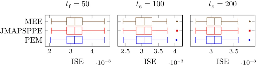
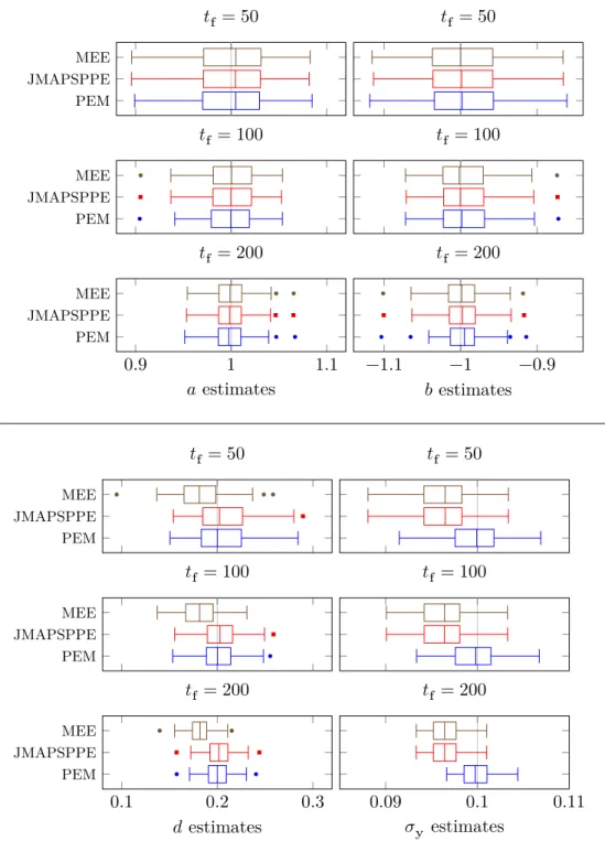
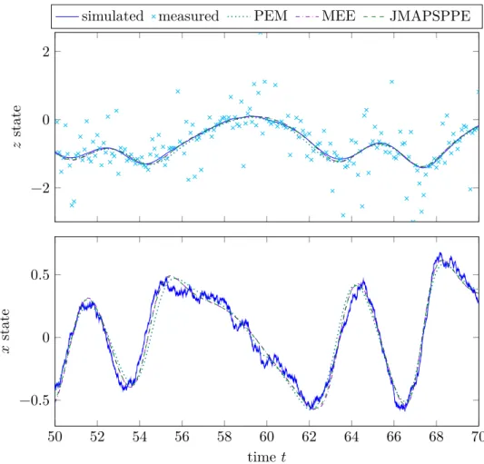
Example applications of the proposed estimators are also shown, with both simulated and experimental data. The MAP and minimum energy estimators are compared with each other and with other popular alternatives.

(10)

(11)

Resumo

Uma grande variedade de fenômenos de interesse para engenharia e ciência são a tempo contínuo por natureza e podem ser modelados por equações diferenciais estocásticas (EDEs), que representam a evolução da incerteza nos estados do sistema. Para sistemas dessa classe, alguns parâmetros da EDE podem ser desconhecidos e os dados coletados frequentemente incluem ruídos, de modo que estimatores de esstados e parâmetros são necessários para realizar inferência e análises adicionais usando a trajetória dos estados do sistema. Uma dessas aplicações é em ensaios em voo de aeronaves, para os quais reconstrução de trajetória de voo ou outras técnicas de suavização são utilizadas antes de se proceder para análise aerodinâmica ou identiﬁcação de sistemas.

As distribuições de EDEs não lineares ou sujeitas a ruído de medição não Gaussiano não admitem expressões analíticas utilizáveis, o que leva a estimadores de estados e parâmetros para esses sistemas a basearem-se em heurísticas como os suavizadores de Kalman estendido eunscented, ou o método de predição de erro utilizando ﬁltros de Kalman não lineares. No entanto, o funcional de Onsager–Machlup pode ser utilizado para obter densidades ﬁctícias conjuntas para trajetórias de estado e parâmetros de EDEs com expressões analíticas.

Nesta tese, um arcabouço teórico unificado é desenvolvido para estimação máxima a posteriori (MAP) de variáveis aleatórias genéricas, possivelmente infinito-dimensionais, e é mostrado como o funcional de Onsager–Machlup pode ser utilizado para a construção do estimador MAP conjunto de trajetórias de estado e parâmetros de EDEs. Também é provado que o estimador de mínima energia, comumente confundido com com o estimador de MAP, obtém as trajetórias de estado associadas às trajetórias deruído MAP. Além disso, é provado que os estimadores conjuntos de trajetória de estados e parâmetros MAP discretizados, que emergiram recentemente como alternativas poderosas para os estimadores de Kalman não lineares, convergem hipograficamente à medida que o passo de discretização diminue. O seu limite hipográfico, no entanto, é o estimador MAP para EDEs quando a discretização trapezoidal é utilizada e o estimador de mínima energia quando a discretização de Euler é utilizada, associando interpretações diferentes a cada estimativa discretizada.

(12)

x Resumo

(13)

Notation

A foolish consistency is the hobgoblin of little minds.

Ralph Waldo Emerson,Self-Reliance

Here is a list of the mathematical typography and notation used throughout this thesis. Most are referenced on ﬁrst use and are standard in the literature, still they are collected here for easy reference. To avoid a notational overload, many representations have a simpler form omitting parameters which can be clearly deduced from the context.

Typographical conventions

We begin with some typographical conventions used to represent diﬀerent mathematical objects. Note that these conventions are sometimes broken when they become cumbersome or deviate from the standard convention of the literature.

Identiﬁng subscripts are typeset upright, e.g., _a, b. Matrices are typeset in uppercase bold, e.g., , , 𝜞 , 𝜱.

Random variables are typeset in uppercase while values they might take are represented in lowercase, e.g., if ∶ 𝛺 → IR is a IR-valued random variable over the probability space (𝛺, , ), then ∈ IRcan be used to represent speciﬁc values it can take. The dependence on the outcome will be omitted when unambiguous.

Sets are typeset in uppercase blackboard bold, e.g., , . -chains are typeset in lowercase blackboard bold, e.g., , .

Time indices of stochastic processes are typeset as subscripts when unambigu-ous, e.g., if ∶ IR × 𝛺 → IRis an IR-valued stochastic process over the probability space (𝛺, , ), then ( , )can be written as _u�( )or _u�. Topological spaces are typeset in uppercase calligraphic, e.g., 𝒜, ℬ.

General symbols

IN ∶= {1, 2, 3, … } is the set of natural numbers (strictly positive integers).

(16)

xiv Notation

IR is the set of real numbers.

IR ₀∶= { ∈ IR | 0} is the set of nonnegative real numbers. IR_>0∶= { ∈ IR | > 0} is the set of strictly positive real numbers. IR ∶= IR ∪ {−∞, ∞} is the extended real number line.

Linear algebra

−1 _{is the inverse of the matrix .}

𝖳 _{is the transpose of the matrix .}

u� is an × identity matrix. The subscript indicating the size might be dropped if it can be deduced from the context.

(u�u�) _{is the element in the th row and th column of the matrix .}

(u�) _{is the th element of the vector .}

Probability and measure theory

(𝛺, , ) is a standard probability space (see Ikeda and Watanabe, 1981, Defn. 1.3.3) on which all random variables are deﬁned.

∈ 𝛺 is the random outcome.

ℬ_u� is the Borel -algebra of the topological space , i.e., the -algebra of subsets of generated by the topology of .

{ _u�}_{u� 0} is a ﬁltration on the probability space (𝛺, , ), i.e., _u� ⊂ _u� ⊂ for all , ∈ [0, ∞)such that .

J , K is the process of quadratic covariation between and .

supp( ) is the support of a measure over a measurable space ( , ℬ_u�), i.e., the set ∈ ℬ_u� of all points whose every open neighbourhood has strictly positive -measure (cf. Ikeda and Watanabe, 1981, Sec. 6.8).

( ) is the indicator function of the set , i.e., ( ) ∶= 1if ∈ , 0if ∉ . In addition, we will use the piece of jargon for -almost all ∈ 𝔼 to say that a property holds for all but a zero-measure subset of an event ∈ , i.e., when the property holds for all ∈ 𝔼\ℕ, whereℕ ∈ is a -null event

(ℕ) = 0.

Analysis

| | is the Euclidean norm of ∈ IRu�_.

(17)

xv

||| ||| ∶= max_u�∈u�‖ ( )‖_u� is the supremum norm of a function ∶ → , also known as the inﬁnity or uniform norm.

, is the inner product between and . If , ∈ IRu�_{, the Euclidean} inner product is implied , ₂∶= 𝖳 _{, unless otherwise speciﬁed by a} subscript.

u�

u�( , , ) is the Banach space of ∶ → IRu� functions endowed with the norm‖ ‖_u�u�

u� ∶= (∫u�‖ ( )‖

u�_{d ( ))}1u�_{, where}_{( , , )}_{is a measure space.}

For ⊂ IRu� _{the Lebesgue -algebra and measure are implied and the} notation may be shortend to u�

u�( ). Additionally, the subscript may be ommited for = 1, i.e., u� _∶= u�

1. 2

u�( , , ) is the Hilbert space of ∶ → IRu� functions endowed with the inner product , _u�2_u� ∶= ∫_u� ( )𝖳 ( ) d ( ), where ( , , ) is a

measure space. For ⊂ IRu� _{the Lebesgue -algebra and measure are} implied and the notation may be shortend to 2

u�( ). Additionally, the superscript may be ommited for = 1, i.e., 2 _∶= 2

1. 2

u�([ , ]) is the Hilbert space of absolutely continuous ∶ [ , ] → IRu� func-tions with square-integrable weak derivatives ∈ 2

u�([ , ]), endowed with the inner product , _u�2_u� ∶= ( )𝖳 ( ) + ∫

u�

u� ( )𝖳 ( ) d , which is the direct sum of copies of the Sobolev space 2,1_{([ , ]).}

𝒞( , ) is the space of continuous functions ∶ → between the topological spaces and . The domain and codomain can be ommited if they can be inferred from the context. If is a compact Hausdorﬀ space, like a closed interval of IR, and = IRu�_{, then}_𝒞_{is assumed to be endowed} with the supremum norm |||⋅|||, unless otherwise noted.

PL(𝒫, ) is the space of piecewise linear functions, with breaks over the partition 𝒫, from [min(𝒫), max(𝒫)]to .

𝜕 , 𝜕 is the boundary of a set or the boundary of a − ℎ . ̄ _{is the closure of a set .}

int is the interior of a set .

∫ ∘ d is the Stratonovich integral of the process with respect to the process .

Miscellaneous

∇_x ( ) ∶= [u�u�(u�)

u�u�(u�)( )]

(u�u�)

is the Jacobian matrix of the function with respect to the input , evaluated at the point .

div_x ( ) ∶= ∑_u� u�u�(u�)_u�u�(u�)( ) is the divergence of the function with respect to

(18)

(19)

List of Acronyms

BVP boundary value problem,

COIN-OR computational infrastructure for operations research, EKF extended Kalman ﬁlter,

EKS extended Kalman smoother, IPOPT interior point optimizer,

JMAPSPPE joint maximuma posteriori state path and parameter estimator, IAE integrated absolute error,

ISE integrated square error, MAP maximuma posteriori, MEE minimum energy estimator, MMSE minimum mean square error, NLP nonlinear program,

ODE ordinary diﬀerential equation, OEM output error method,

PEM prediction error method, SDE stochastic diﬀerential equation, UKF unscented Kalman ﬁlter, UKS unscented Kalman smoother,

UFMG Universidade Federal de Minas Gerais.

(20)

(21)

Chapter 1

Introduction

The subject of this thesis is joint maximum a posteriori state path and param-eter estimation in systems described by stochastic differential equations, and its main contribution is the introduction of two new estimators. Besides their obvious use in joint state path parameter estimation, the proposed estimators can also be employed in system identification and in smoothing, i.e., in appli-cations where both the parameters of the system and its states are unknown but either only the parameters or the states are sought after. Consequently, this thesis is concerned not only with the intersection of parameter and state estimation, but also with each of these fields of study independently.

We begin this chapter with an overview of smoothing and dynamical system parameter estimation, presented in Section 1.1, covering both their historical developments and the state of the art. We then proceed to present the motivation, objectives and contributions of this thesis in Section 1.2.

1.1 A brief survey of the related literature

In this section we present a brief survey of the literature related to the top-ics investigated herein. We begin by presenting important deﬁnitions and terminology which will be used throughout this thesis.

1.1.1 Classes of models and state estimation

To best estimate quantities associated with dynamical systems from measure-ments spread out over time, the measured values should be used in conjunction with knowledge of the system dynamics. This is especially important when both the measurements and the dynamics are uncertain, and described by a stochastic model instead of deterministic functions. Taking into account that for most real-world systems all models are approximations and all measure-ments have ﬁnite precision, models that take into account these shortcomings are more realistic than those that do not.

(22)

2 Chapter 1. Introduction

time

signals

discrete-time

state meas.

time continuous-time

state meas.

time

continuous–discrete

state meas.

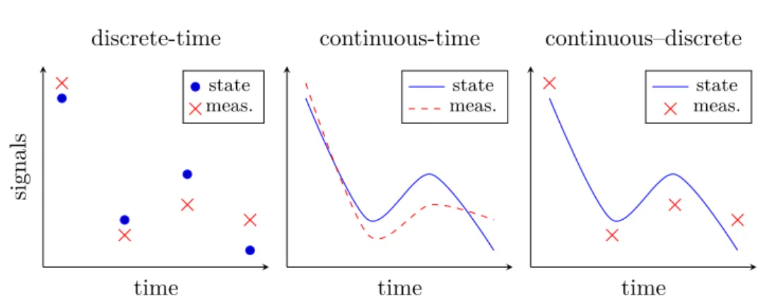
Figure 1.1: Graphical representation of the state and measurements for the three model classes.

The uncertainty in stochastic dynamical models can be due to unknown external disturbances acting on the system or can be simply a way for the modeler to express his lack of conﬁdence and repeatability on the outcomes of the system. Examples of random external disturbances include electromag-netic interference in a circuit, thermal noise in a conductor, turbulence in an airplane and solar wind in a satellite, to name a few. Whether the behavior of the system—or of the corresponding disturbances—is truly random does not matter, stochastic models for dynamical systems are an important tool to make inference taking into account the uncertainties involved in the dynamics and data acquisition. These tools can be used with both the subjectivist and ob-jectivist Bayesian points of view (for more information on these interpretations and their dichotomy see Press, 2003, Chap. 1).

Stochastic models for dynamical systems can be classiﬁed into three major classes, according to how the dynamics and measurements are represented (cf. Jazwinski, 1970, p. 144):

discrete-time models are those in which both the measurements and the under-lying system dynamics are represented in discrete-time, over a possibly inﬁnite but countable set of time points;

continuous-time models are those in which both the measurements and the underlying system dynamics are represented in continuous-time, over an uncountable set of time points;

continuous–discrete models, also known as sampled-data or hybrid models, are those in which the measurements are taken in discrete-time but the underlying system dynamics is represented in continuous-time. The measurements times are then a countable subset of the time interval over which the dynamics is represented.

(23)

1.1. A brief survey of the related literature 3

time

measurements most recent

initial

times of interest

smoothing ﬁltering prediction

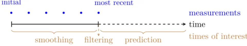
Figure 1.2: Graphical representation of the classes of state estimation.

and engineering are of a continuous-time nature, yet the measurements available for inference are sampled at discrete time instants.

The dynamics of discrete-time systems are usually represented by sto-chastic difference equations. Likewise, the dynamics of continuous-time and continuous–discrete systems are usually represented by stochastic differential equations (SDEs). Models represented by SDEs are used to make inference in a wide range of applications, including but not limited to radar tracking (Arasaratnam et al., 2010), aircraft flight path reconstruction (Mulder et al., 1999) and investment finance and option pricing (Black and Scholes, 1973); see the reviews by Kloeden and Platen (1992, Chap. 7), and Nielsen et al. (2000) for a comprehensive list.

In a very influential article, Kalman (1960) defined three related classes of estimation problems for signals under noise, given measurements spread out over time. His definitions are now standard terminology, and consist of the following classes:

ﬁltering, where the goal is to estimate the signal at the time of the latest measurement;

prediction, also known as extrapolation or forecasting, where the goal is to estimate the signal at a time beyond that of the latest measurement; smoothing, also known as interpolation, where the goal is to estimate the

signal over times up to that of the latest measurement.

The ﬁltering and prediction problem usually arise in online (real-time) ap-plications, such as process control and supervision. The smoothing problem, on the other hand, arises in oﬄine (post-mortem, after the fact) applications, or online applications where a delay between measurement and estimation is tolerable. In smoothing, future data (with respect to the estimate) is used to obtain better estimates (Jazwinski, 1970, p. 143). These classes are represented graphically in Figure 1.2.

Three additional subclasses of the smoothing problem were deﬁned by Meditch (1967) and have also been adopted into the jargon:

(24)

ﬁxed-point smoothing, where the goal is to estimate the signal at a speciﬁc time-point before the latest measurement;

ﬁxed-lag smoothing, where the goal is to estimate the signal at a speciﬁc time-distance from the latest measurement.

The difference between fixed-point and fixed-lag smoothing is only relevant in online applications.

In the context of Bayesian statistics, the smoothing estimates are usually chosen as the posterior mean or the posterior mode. The posterior mean is known as the minimum mean square error (MMSE), as it minimizes the expected square error with respect to the true states, over all outcomes for which the measured values would have been observed. The posterior mode is known as the maximuma posteriori (MAP) estimate, as it maximizes the posterior density. It is interpreted as the most probable outcome, given the measurements. Fixed-interval MAP smoothing can, furthermore, be divided into two classes:

MAP state-path smoothing, where the estimates are the joint posterior mode of the states along all time instants in the interval, given all the mea-surements available;

MAP single instant smoothing, where the estimate for each time instant is the marginal posterior mode of the state at the instant, given all the measurements available.

Godsill et al. (2001) refer to these classes as the joint and marginal MAP estimation. The MAP state-path smoothing is also referred to as MAP state-trajectory smoothing or, in the discrete-time case, MAP state-sequence smoothing. As there is not much literature on this class of estimators, the terminology is not well cemented.

1.1.2 Smoothing

The modern theory of smoothing has its origins in the works of Wiener (1964)1 and Kolmogorov (1941)2_{, who developed the solution to stationary linear} systems subject to additive Gaussian noise. Wiener solved the continuous-time problem while Kolmogorov solved the discrete-time one. Their approach used the impulse response representation of systems to derive the results and represent the solutions. Wiener’s work seems to have pioneered the use of statistics and probability theory to both formulate and solve the problem of ﬁltering and smoothing of signals subject to noise.

(25)

the seminal work of Kalman (1960), who solved the problem of non-stationary estimation in linear discrete-time and continuous–discrete systems subject to additive Gaussian noise. The Kalman filter differed significantly from the Wiener filter by the use of the state-space formulation in the time domain to derive the results and represent the solution. Shortly after, Kalman and Bucy (1961) proposed the Kalman–Bucy filter, the analog of the Kalman filter for continuous-time systems with continuous-time measurements. It should be noted that for linear–Gaussian systems there existexact formulas for the discretization, so there is little difference between the discrete-time and continuous–discrete formulations.

In his initial paper, Kalman (1960) mentions that smoothing falls within the theory developed, but he does not address the smoothing problem directly. The Kalman filter was, however, readily extended to solve the smoothing problem by Bryson and Frazier (1963) for the continuous-time case, and by Cox (1964) and Rauch et al. (1965)3 _{for the discrete-time case. The above} mentioned smoothers work by combining the results of a standard forward Kalman filter with a backward smoothing pass, which led to them being classified as forward–backward smoothers. Another approach, introduced by Mayne (1966), consists of combining the results of two Kalman filters, one running forward in time and another one running backward, which came to be called two-filter smoothing.

The two-filter and forward backward smoothers can also be adapted to general nonlinear systems and to non-Gaussian systems. However, in these genearal cases, the smoothing distributions do not admit known closed-form expressions, except in some very specific cases. For these systems, consequently, practical smoothers must rely on approximations. One of the first of these approximations was the linearization of the system dynamics, which led to the development of the extended Kalman filter and smoothers (for a historical perspective on its development see Schmidt, 1981).

Nonlinear Kalman smoothers like the extended Kalman smoother follow roughly the same steps as their linear counterparts, summarizing the relevant distributions by their mean and variance. This implies that their underlying assumption is that the densities involved in the smoothing problem are ap-proximately Gaussian. Consequently, the two-ﬁlter Rauch–Tung–Striebel or Bryson–Frazier formulas can be used if appropriate linear–Gaussian approx-imations are made. Besides the extended Kalman approach of linearization by truncating the Taylor series of the model functions, other approaches to obtain linear–Gaussian approximations include the unscented transform (Julier and Uhlmann, 1997), the statistical linear regression (Lefebvre et al., 2002) or Monte Carlo methods (Kotecha and Djuric, 2003), to name a few. The unscented Kalman ﬁlter of Julier and Uhlmann (1997), in particular, was

(26)

formalized for smoothing with the two-ﬁlter formula by Wan and van der Merwe (2001, Sec. 7.3.2) and with the Rauch–Tung–Striebel forward–backward correction by Särkkä (2006, 2008).

More general smoothers for nonlinear systems are based on non-Gaussian approximations of the smoothing distributions. The two-filter smoother of Kitagawa (1994), for example, uses Gaussian mixtures to represent the dis-tributions and the Gaussian sum filters of Sorenson and Alspach (1971) to perform the estimation. Sequential Monte Carlo two-filter (Kitagawa, 1996; Klaas et al., 2006) and forward–backward smoothers (Doucet et al., 2000; Godsill et al., 2004) represent the distributions by weighted samples using the sequential importance resampling method of Gordon et al. (1993). Sequential Monte Carlo methods can also be used for MAP state-path smoothing by employing a forward filter in conjunction with the Viterbi algorithm to select the most probable particle sequence, as proposed by Godsill et al. (2001).

MAP state-path smoothers, nevertheless, do not need to be formulated or implemented in the sequential Bayesian estimator framework. For a wide variety of systems, the posterior state-path probability density admits tractable closed-form expressions4 _{which can be easily evaluated on digital computers.} Therefore, by the use of nonlinear optimization tools, the MAP state-path can be obtained without resorting to Bayesian ﬁlters.

Since the early developments in Kalman smoothing, MAP state-path esti-mation by means of nonlinear optimization was considered as a generalization of linear smoothing to nonlinear systems subject to Gaussian noise (Bryson and Frazier, 1963; Cox, 1964; Meditch, 1970). However, the limitation of the computers available at the time meant that the estimates could not be obtained by solving a single large-scale nonlinear program. Therefore, the division of the large problem into several small problems, as performed by the extended Kalman smoother, was advantageous. Furthermore, for discrete-time systems, the extended Kalman smoother was shown (Bell, 1994; Johnston and Krishnamurthy, 2001) to be equivalent to Gauss–Newton steps in the maximization of the posterior state-path density. Because of those similarities, the terminology is still not standard, with many diﬀerent methods falling under the umbrella of Kalman smoothers. In this thesis, we will refer to asnonlinear Kalman smoothersthose methods which rely on two-ﬁlter or forward–backward formulas, and as MAP state-path smoothers those methods which rely on nonlinear optimization to obtain their estimates.

As the tools of nonlinear optimization matured, optimization-based MAP state-path smoothers emerged again as powerful alternatives to nonlinear Kalman smoothers (Aravkin et al., 2011, 2012a,b,c, 2013; Bell et al., 2009; Dutra et al., 2012, 2014; Farahmand et al., 2011; Monin, 2013). Furthermore, unlike nonlinear Kalman smoothers, these smoothers are not limited to

(27)

tems with approximatelly Gaussian distributions, which lends them a wider applicability. It also opens the possibility to model the systems with non-Gaussian noise. Heavy-tailed distributions are often used to add robustness to the estimator against outliers, even when the measurements actually come from a diﬀerent distribution. Examples of robust MAP state-path smoothing with heavy-tailed distributions include the work of Aravkin et al. (2011) and Farahmand et al. (2011) with the ℓ₁-Laplace, and the work of Aravkin et al. (2012a,c) with piecewise linear-quadratic log densities and Student’s . Distri-butions with limited support, such as the truncated normal, can also be used to model constraints (Bell et al., 2009).

One theoretical issue with MAP state-path smoothing that persisted up to recently was its correct definition, interpretation, and formulation for continuous-time or continuous–discrete systems, and the applicability of discrete-time methods to discretized continuous systems. The definition is not trivial because the state-paths of these systems lie in infinite-dimensional separable Banach spaces, for which there is no analog of the Lebesgue measure, i.e., a locally finite, strictly positive and translation-invariant measure. Conse-quently, the measure-theoretic definition of density as the Radon–Nikodym derivative of the probability measure is not applicable for the purposes of obtaining the posterior mode (Dürr and Bach, 1978, p. 155).

Nevertheless, systems described by stochastic differential equations do possess asymptotic probability of small balls, given by the Onsager–Machlup functional. This functional, first derived by Stratonovich (1971) for nonlinear SDEs, can be thought of as an analog of the probability density for the purpose of defining the mode. In the statistics and physics literature, a consensus arose that the maxima of the Onsager–Machlup functional represented the most probable paths of diffusion processes (Dürr and Bach, 1978; Ito, 1978; Takahashi and Watanabe, 1981; Ikeda and Watanabe, 1981, Sec. VI.9; Hara and Takahashi, 1996) and that it should be used for construction of MAP state-path estimators (Zeitouni and Dembo, 1987).

Despite that, in the automatic control and signal processing literature, the Onsager–Machlup functional seemed to be virtually unknown until the late 20th century. One of the few uses of the Onsager–Machlup functional for MAP state-path estimation in the engineering literature was the work of Aihara and Bagchi (1999a,b), which did not enjoy much popularity.5 _{In fact,} as is detailed in the next paragraph, many authors incorrectly obtained the energy functional as the merit function for MAP state-path estimation. The energy functional diﬀers from the Onsager–Machlup functional by the lack of a correction term which, when ommitted, can lead to diﬀerent estimates.

Cox (1963, Chap. III), for example, obtained the energy functional by

5_{Only one citation from other authors, up to 2013, was found for both these articles in}

(28)

applying the probability density functional of Parzen (1963) to the driving noise of the SDE, without taking into account that the nonlinear drift might cause the mode of the state path to differ from the mode of the noise path, as proved to be the case in Chapter 2 of this thesis and in one of its derivative works (Dutra et al., 2014). Mortensen (1968) obtained the energy functional by Feynman path integration in function spaces, but apparently used an incorrect integrand, as the Onsager–Machlup function is the correct Lagrangian in the path integral formulation of diffusion processes (Graham, 1977).6 _Jazwinski (1970, p. 155), on the other hand, obtained the energy by considering the limit of the mode of the Euler-discretized systems. However, as argued by Horsthemke and Bach (1975), the Euler discretization cannot be used for such purposes due to insufficent approximation order.

The recent renewed interest in MAP state-path estimators, afforded by the maturity of the necessary optimization tools, focused mostly on discrete-time systems. When applied to continuous-discrete systems described by SDEs, discretization schemes were used, as done by Bell et al. (2009) and Aravkin et al. (2011, 2012c). For nonlinear systems, SDE discretization schemes are ap-proximations which improve as the discretization step decreases. Applications in Kalman filtering that use such discretization schemes, for example, usually require fine discretizations to produce meaningful results (Arasaratnam et al., 2010; Särkkä and Solin, 2012). An important requirement for the adoption of discrete-time MAP state-path smoothing for discretized continuous-time systems is then understanding if and how the discretized MAP state path relates to the MAP state path of the original system.

In this thesis we proved that, under some regularity conditions, discretized MAP state-path estimation converges hypographically to variational estimation problems, as the discretization step vanishes. However, the limit depends on the discretization scheme used. For the Euler discretization scheme, the most popular, the discretization converges to the minimum energy estimation, which is proved to correspond to the state path associated with the MAP noise path. When the trapezoidal scheme is used, on the other hand, the estimation converges to the MAPstate-path estimation using the Onsager–Machlup func-tional. Our work also offers a formal definition of mode and MAP estimation of general random variables in possibly infinite-dimensional spaces, under the framework of Bayesian decision theory. Finally, it highlights the links between continuous–discrete MAP state-path estimation and optimal control, opening up an even wider range of tools for this class of estimation problems. These results were published in a derivative work of this thesis (Dutra et al., 2014). Having layed down a solid theoretical foundation for MAP state-path estimation in systems described by SDEs, the field is now ripe for its use

6_{The exact integrand used could not be found, as the derivation was performed in}

(29)

in non-Gaussian applications, such as robust smoothing, and ﬁelds typically dominated by nonlinear Kalman smoothing, such as aircraft ﬂight path recon-struction (Mulder et al., 1999; Jategaonkar, 2006, Chap. 10; Teixeira et al., 2011).

1.1.3 System identiﬁcation

System identiﬁcation is the inverse problem of obtaining a description for the behavior of a system based on observations of its behavior. For dynamical systems, the system is represented by a suitable mathematical model and the observations are measured input–output signals of its operation. The process of dynamical-system identiﬁcation is often structured as composed of four main tasks:

data collection, the process of planning and executing tests to obtain repre-sentative observations of the system dynamics;

model structure determination, the process of choosing a parametrized struc-ture and mathematical representation for the model, using both a priori information and some of the collected data;

parameter estimation, the process of obtaining parameter values from the collected data and prior knowledge;

model validation, the process of evaluating if the chosen model with its esti-mated parameters is an adequate description of the system.

Each of these tasks is dependent upon the preceding ones, but the overall process can be iterative and involve multiple repetitions until a suitable combination of data, model, and parameters is found.

With respect to the model structure, three main classes are usually consid-ered:

white-box models, also known as phenomenological models, constructed from ﬁrst principles and knowledge of the system internals;

black-box models, also known as behavioral models, of a general structure chosen to represent the input–output relationship without regard to the system internals;

grey-box models, those which combine aspects of both white- and black-box models, featuring components whose dynamics are derived from ﬁrst principles and others whose dynamics only represent some cause–eﬀect relationship.

(30)

descriptions of the dynamics of most systems are formulated in continuous-time. Additionally, the representation of the state dynamics by stochastic differentential equations is a valuable tool for grey-box modelling, as it can put together a simplified phenomenological representation with a source of uncertainty that accounts for the simplifications performed (cf. Kristensen et al., 2004a,b).

1.1.4 Parameter estimation in stochastic diﬀerential equations

In the process of system identification, parameter estimation can be thought of as procedures for extracting the information from the data. For systems for which the states are directly observable, without measurement noise, the field is well-consolidated and there exist a plethora of estimation techniques; see Nielsen et al. (2000, Secs. 3–4) and Bishwal (2008) for reviews. However, while the assumption of no measurement noise might be realistic for stock market and finantial modelling, it is overly optimistic for most engineering applications. When measurement noise is considered, the estimation problem becomes more complex and the field is still under active development.

In the remainder of this section, we will focus only on methods and tech-niques which take measurement noise into account. As the states are not directly measured, this class of parameter estimators is closely related to state estimators. Intuitively thinking, to model the evolution of the states one ﬁrst needs estimates of their values.

For Markovian systems, the likelihood function can be decomposed into the product of the one-step-ahead predicted output densities, given all previous measurements, evaluated at the measured values. Consequently, for linear systems subject to Gaussian noise, the likelihood function can be obtained by employing a Kalman filter to obtain the predicted output distributions. This approach was pioneered by Mehra (1971) and came to be known as the prediction-error method or filter-error method. Among its first applications was the parameter estimation of aircraft models from flight-test data collected under turbulence (Mehra et al., 1974). These methods can be used for both maximum likelihood and maximuma posteriori parameter estimation; see the survey by Åström (1980) for a review of its early developments.

(31)

or particle filters (Andrieu et al., 2004; Doucet and Tadić, 2003), can be used in prediction error methods. The limitations and difficulties associated with these methods are, likewise, those of their underlying nonlinear filters. Furthermore, the performance of the filters is usually significantly degraded when the parameters are far from the optimum, which can make the estimator sensitive to the initial guess.

Another popular approach for parameter estimation worth mentioning consists of treating parameters as augmented states and using standard state estimation techniques (see Jazwinski, 1970, Sec. 8.4; or Ljung, 1979, and the references therein). These methods have the serious disadvantage, however, that if no process noise is assumed to act on the augmented states corresponding to the parameters, their estimated variance will converge to zero. Given all the approximations involved, that is overly optimistic and, furthermore, can cause the estimators to fail. Consequently, a small artificial noise is assumed to act on the dynamics of, but this workaround also introduces its own drawbacks. The choice of the parameter noise variance is difficult and its effect on the original problem is not always clear. Also, the final output of the method is not a single estimate for the parameters but a time-varying one. It is not obviuos how to choose one instant or combine the estimate a different instants to obtain the best value.

Up to the early 21st century, not much new development was done in parameter estimation in systems described by SDEs subject to measurement noise, as argued by Kristensen et al. (2004b, p. 225). A review by Nielsen et al. (2000) pointed to the decades-old prediction error method with the extended Kalman ﬁlter as the most general and useful approach at the time for parameter estimation in this class of systems.

A new development came in the work of Varziri et al. (2008b), which they termed the approximate maximum likelihood estimator. As explained in (Varziri et al., 2008a, p. 830), their estimator can be interpreted as a joint MAP state-path and parameter estimator with a non-informative parameter prior. If the state-path and parameter posterior is then approximately jointly symmetric, the estimated parameter should be close to the true maximum likelihood estimate. However, it should be noted that they used the energy functional, as derived by Jazwinski (1970, p. 155), instead of the Onsager–Machlup functional to construct their merit function. This means that their estimates have a diﬀerent interpretation than intended, as is proved in Chapter 2 of this thesis. In Chapter 3 of this thesis we prove, furthermore that their derivation would be the one intended if the trapezoidal discretization scheme had been used instead of the Euler scheme.

(32)

heuristics (Karimi and McAuley, 2014b; Varziri et al., 2008c). However, a more rigorous and promising approach is using the Laplace approximation to marginalize the states in the joint state-path and parameter density to obtain an approximation of the parameter likelihood function (Karimi and McAuley, 2013, 2014a; Varziri et al., 2008a). In this context, the Laplace approximation is a technique to marginalize the state-path out of the posterior joint state-path and paremeter density, obtaining the posterior parameter density. It consists of making a Gaussian approximation of the state-path at its mode from the Hessian of the log-density. It should be noted that the assumption that the posterior state-path smoothing distribution is approximately Gaussian is usually less strict than the assumption that the one-step-ahead predicted output is approximately Gaussian.

Once again, these estimators used the energy functional instead of the Onsager–Machlup functional, implying that they are, in fact, applying the Laplace approximation to marginalize the noise path out of the joint noise-path and parameter distribution. The noise-path is usually less observable than the state-path, implying that the Hessian of its log-posterior usually has a smaller norm and the Laplace approximation is coarser. We also remark that, although easily adapted to non-Gaussian measurement and prior distributions, the literature on these estimators is restricted to the case where these distributions are all Gaussian (Karimi and McAuley, 2013, 2014a,b; Varziri et al., 2008a,b; Varziri et al., 2008c).

We can then see that joint MAP state-path and parameter estimators figure as an important tool for further development in parameter estimators for systems described by stochastic differential equations. However, theoretical difficulties with the correct definition of MAP state-path and the effects of discretizations must be clearly resolved for these methods to gain a wider adoption. Once these issues are resolved, these estimators can be used in applications dominated by nonlinear-Kalman prediction-error methods and non-Gaussian applications. In particular, just like with MAP state-path estimation, heavy-tailed distributions can be used to perform robust system identification in the presence of outliers.

1.2 Purpose and contributions of this thesis

(33)

1.2. Purpose and contributions of this thesis 13

1.2.1 Motivations

The motivations of this thesis are twofold: a technological driver based on demand from applications; and the need to better understand the theory behind maximum a posteriori state-path and joint state-path and parameter estimation in systems described by stochastic diﬀerential equations. Inportant theoretical considerations that need a better understanding are the probabilistic interpretations of the minimum energy and MAP joint state-path and parameter estimators and their relationship to the discretized estimators.

TheUniversidade Federal de Minas Gerais7 _{(UFMG) is one of the} lead-ing centers of aeronautical technology research and education in Brazil. Its activities encompass all aspects of aeronautical engineering, including desing, construction and operation of airplanes and aeronautical systems. Among its current projects are a light airplane with assisted piloting, a racing airplane to beat world speed records, and hand-lauched autonomous unmanned aerial vehicles.

Flight testing is an integral part of design and operation of aircraft and aeronautical systems. Its purposes include analysis of aircraft performance and behaviour; identification of dynamical models for control and simulation; and testing of systems and algorithms. Flight test data is subject to noise and sensor imperfections; it is typically preprocessed before any analysis is done. The process of recovering the flight path from test data is known as flight-path reconstruction (Mulder et al., 1999; Jategaonkar, 2006, Chap. 10; Klein and Morelli, 2006, Chap. 10) and is an essential step for flight-test data analysis. In adition, flight vehicle system identification is an indispensable tool in aeronautics with great engineering utility; see the editorial by Jategaonkar (2005) from the special issues of the Journal of Aircraft on this topic and some of the reviews therein (Jategaonkar et al., 2004; Morelli and Klein, 2005; Wang and Iliff, 2004) for more information.

Small hand-launched unmanned aerial vehicles, like the ones being de-signed and operated at UFMG, present additional challenges to flight-path reconstruction and system identification. Their small payload limits the weight of the flight-test instrumentation that can be carried onboard, restricting the instrumentation to lightweight sensors with more noise, bias and imperfections. Their small weight also makes them more sensitive to turbulence, which needs to be accounted for. The technological motivation of this thesis is then to develop state and parameter estimators for flight-path reconstruction and system identification which are appropriate for use in small hand-launched unmanned aircraft.

Related to our technological motivation, we have that the tools of MAP state-path estimation, which show great promise for our intended application,

(34)

still has an unclear definition for systems described by stochastic differential equations. Furthermore, the relationship between discretized estimators and the continuous-time underlying problem needs to be understood with a rigorous mathematical analysis. Consequently, our theoretical motivations are to provide a firm theoretical basis for MAP state-path and parameter estimation in continuous-time and continuous–discrete systems.

1.2.2 Objectives and contributions

Having stated the motivations behind this work, the objectives of this thesis are then

• to provide a rigorous definition of mode and MAP estimation for random variables in possibly infinite-dimensional spaces which coincides with the usual definition for continuous and discrete random variables;

• to derive the joint MAP state-path and parameter estimator for systems described by SDEs, together with conditions and assumptions for its applicability;

• to obtain a probabilistic interpretation for the joint minimum energy state-path and parameter estimator, together with conditions and as-sumptions for its applicability;

• to relate discretized joint MAP state-path and parameter estimators to their continuous-time counterparts;

• to demonstrate the viability of the derived estimators in example appli-cations with both simulated and experimental data.

We believe these are important steps for further advancement of the ﬁeld and the use of these techniques in novel and challenging applications.

The speciﬁc contributions and novelties of this thesis are

• formalization of the concept of ﬁctitious densities, in Deﬁnition 2.4; • formalization of the concept of mode and MAP estimator for random

variables in metric spaces, using the concept of ﬁctitious densities, in Proposition 2.6 and Deﬁnitions 2.5 and 2.7;

• derivation of the Onsager–Machlup functional for systems with unknown parameters and possibly singular diﬀusion matrix, in Theorem 2.9; • probabilistic interpretation of the energy functional as the ﬁctitious

den-sity of the associated noise path, in Theorem 2.26, extending the results published in (Dutra et al., 2014) to systems with unknown parameters and possibly singular diﬀusion matrices;

(35)

1.3. Outline of this thesis 15

2014) to systems with unknown parameters and possibly singular diﬀusion matrices.

1.3 Outline of this thesis

(36)

(37)

Chapter 2

MAP estimation in SDEs

Don’t panic!

Douglas Adams,The Hitchhiker’s Guide to the Galaxy

This chapter contains the main theoretical contributions of this thesis. We begin with the deﬁnition and interpretations of maximum a posteriori (MAP) estimation in Section 2.1, and then proceed to apply the concepts developed for the derivation of the joint MAP state-path and parameter estimator for systems described by stochastic diﬀerential equations (SDEs) in Section 2.2. Then, in Section 2.3, the joint MAP noise-path and parameter estimator is derived and shown to be the minimum energy estimator obtained by omitting the drift divergence in the Onsager–Machlup functional.

2.1 Foundations of MAP estimation

In this section, we present the theoretical foundations of maximuma posteriori (MAP) estimation. We begin with a brief presentation of Bayesian point estimation and show how some parameters of the posterior distribution, such as the mean and mode, are the Bayesian estimates associated with popular loss functions. We then define the mode of discrete and continuous random variables over IRu� and extend this definition to random variables over general metric spaces, like paths of stochastic processes. The MAP estimator is then defined as the posterior mode and interpreted in the context of Bayesian decision theory.

2.1.1 General Bayesian estimation

In Bayesian statistics, the posterior distribution of a random quantity of interest, given an observed event, is the aggregate of all the information available on the quantity (Migon and Gamerman, 1999, p. 79). This information is represented in the form of a probabilistic description, and includes the prior,

(38)

18 Chapter 2. MAP estimation in SDEs

what was known before the observation, and the likelihood, what is added by the observation. This information can be used to make optimal decisions in the face of uncertainty, with the application of Bayesian decision theory.

In Bayesian decision theory, a loss function is chosen to represent the undesirability of each choice and random outcome. The Bayesian choice is then that which minimizes the expected posterior loss, over all possible decisions (Robert, 2001). Alternatively, the problem can be modeled in terms of the gain associated with each choice and random outcome, in which case the Bayesian choice is the one which maximizes the expected posterior gain. Gain functions are also refered to as utility functions.

One application of Bayesian decision theory is Bayesian point estimation. Although any summarization of the posterior distribution leads to some loss of information, it is often necessary to reduce the distribution of a random variable to a single value for some reason, among them reporting, communication or further analysis which warrants a single, most representative, value. A loss function is then used to quantify the suitability of each estimate, for each possible outcome of the random variable of interest, and the point estimate is the choice which minimizes the expected posterior loss. This concept is detailed below.

Let be an -valued random variable of interest and be a -valued observed random variable. An estimator is a deterministic rule ∶ → to obtain estimates for given observed values of . The performance of estimators is compared using measurable loss functions ∶ × → IR 0. For each outcome = , ( ̂, )evaluates the penalty (or error) associated with estimate ̂. The integrated risk (or Bayes risk) associated with each estimator is then deﬁned by

( ) ∶= E[ ( ( ), )] ,

whereE[⋅]denotes the expectation operator. The risk is the mean loss over all possible values of the variable of interest and the observation. Having chosen an appropriate loss function for the problem at hand, the Bayesian estimators are deﬁned as follows.

Deﬁnition 2.1 (Bayesian estimator). A Bayesian estimator b_{∶ →} _for

the random variable , associated with the loss function , given the observed value ∈ of , is any which minimizes the expected posterior loss, i.e.,

E[ ( b_{( ), ) ∣ = ] = min}

u�∈u�E[ ( , ) | = ] .

(39)

2.1. Foundations of MAP estimation 19

exist several choices which are indistinguishable with respect to that criterion. In addition, if a Bayesian estimator exists for _u�-almost everywhere , then it attains the lowest possible integrated risk (Robert, 2001, Thm. 2.3.2).

One way to interpret these quantities is making an analogy to a game of chance. The estimate ̂is a bet on the value of , given that the player knows = about the state of the game. The estimator represents a betting strategy and the loss function the financial losses for each outcome and bet, that is, the payoff. The integrated risk is then the average loss expected for a given betting strategy. Thus, an optimal betting strategy would minimize the integrated risk, leading to the minimum financial losses in the long run.1

There exist many canonical loss functions whose Bayesian estimators are certain statistics of the posterior distribution. Take, for example, quadratic error losses:

2( ̂, ) ∶= ℎ( − ̂, − ̂),

where ℎ∶ × → IR ₀ is a coercive and bounded bilinear functional. For = IRu� thenℎ is a positive-deﬁnite quadratic form, i.e.,

2( ̂, ) = ( − ̂)𝖳 ( − ̂)

for any positive deﬁnite ∈ IRu�×u�. The Bayesian estimator associated with this family of loss functions is the posterior mean of . This result was proved for IR-valued random variables by Gauss and Legendre (see Robert, 2001, Sec. 2.5.1) but also holds, under some regularity assumptions, when is a more general reﬂexive Banach space.

A similar result holds for the absolute error loss,

1( ̂, ) ∶= ‖ ̂ − ‖ .

When is an absolutely integrable IR-valued random variable, then the Bayesian estimator associated with the ₁ loss is is the posterior median, a result initially proved by Laplace (see Robert, 2001, Prop. 2.5.5). When is IRu�_{-valued and} _{E[| | | = ] < ∞, then the posterior spatial median (also} known as the ₁-median) is the Bayesian estimator associated with the ₁ loss. This concept also generalizes well to inﬁnite-dimensional–valued ; the spatial median is also the Bayesian estimator associated with the ₁ loss when

is a reﬂexive Banach space (Averous and Meste, 1997).

The modes, which are known as maximuma posteriori estimates, are only degenerate Bayesian estimates, however, for random variables over general 1_{The requirement of}_{u� ≥ 0} _{would not attract many gamblers to the game, however,}

(40)

spaces. Nevertheless, they can be interpreted in the framework of Bayesian decision theory and Bayesian point estimation. Before showing how MAP estimation fits into this framework, we present in the following subsection the formal definition of modes for random variables over possibly infinite-dimensional spaces.

2.1.2 Modes of random variables

The modes of a random variable are population parameters that correspond to the region of the variable’s sample space where the probability is most concentrated. For discrete random variables, i.e., when there is a countable subset of the variable’s sample space with probability one, then the modes are its most probable outcomes. For continuous random variables overIRu�_{, i.e.,} those whose probability measure admits a density with respect to the Lebesgue measure, all individual outcomes of the random variable have probability zero, so the modes are deﬁned as the densest outcomes (Prokhorov, 2002). These deﬁnitions are formalized below.

Deﬁnition 2.2 (modes of discrete random variables). Let be an -valued

random variable such that there exists a countable set ⊂ with _u�( ) = 1. The modes of are the points ̂ ∈ satisfying

( = ̂) = max

u�∈u� ( = ), at least one which exists.

Deﬁnition 2.3 (modes of continuous random variables). Let be an

IRu�-valued random variable that admits a continuous density ∶ IRu�→ IR 0 with respect to the Lebesgue measure. The modes of , if they exist, are the points ̂ ∈ IRu� _satisfying

( ̂) = max u�∈IRu� ( ).

We note that Deﬁnition 2.3 is restricted to random variables with continuous densities because otherwise the deﬁnition is ambiguous. Any function which is equal Lebesgue-almost everywhere to a probability density function is also a density for the same random variable. If the random variable admits a continuous density, then the continuous one is considered as the best density, as it is the one with the largest Lebesgue set and coincides everywhere with the Lebesgue derivative of the induced probability measure (Stein and Rami, 2005, p. 104). If the random variable only admits discontinuous densities, however, then it is not clear which density is the best and should be used for calculating the mode.

(41)

paths of IRu�_{-valued diffusions, there is no analog of the Lebesgue measure,} i.e., a translation-invariant, locally finite and strictly positive measure. Any translation-invariant measure on an infinite-dimensional separable Banach space would assign either infinite or zero measure to all open sets. Thus any measure with respect to which a density (Radon–Nikodym derivative) is taken would weight equally-sized2 _{neighbourhoods differently. Similar problems arise} in more general metric spaces, like the space of paths of diffusion processes over manifolds (cf. Takahashi and Watanabe, 1981).

This limitation is overcome by using a functional that quantifies the con-centration of probability in the neighborhood of paths but, unlike the density, cannot be used to recover the probability of events via integration. The con-centration is quantified by the asymptotic probability of metric 𝜖-balls, as 𝜖 vanishes. The normalization factor of this asymptotic probability weights balls of equal radius equally. Stratonovich (1971), who first proposed these ideas, called it the probability density functional of paths of diffusion processes. We believe, however, that the nomenclature of Takahashi and Watanabe (1981) is more appropriate: the functional is anideal density with respect to afictitious uniform measure 3_{. Zeitouni (1989) shortened this nomenclature to}_fictitious density, which is the term that is used in this thesis. This concept is formalized below.

Deﬁnition 2.4 (ﬁctitious density). Let be an -valued random variable,

where ( , ) is a metric space. The function ∶ → IR ₀ is an ideal density with respect to a ﬁctitious uniform measure, or a ﬁctitious density for short, if there exists ∶ IR_>0→ IR_>0 such that

lim u�↓0

( ( , ) < 𝜖)

(𝜖) = ( ) for all ∈ (2.1)

and ( ) > 0 for at least one ∈ .

Both probability mass functions and continuous probability density func-tions are fictitious densities, according to Definition 2.4. As the modes of discrete and continuous random variables are the location of the maxima of the fictitious density, it is natural to define the mode of general random variables that admit a fictitious density as the location of the maxima of the fictitious densities.

Deﬁnition 2.5 (mode in metric spaces). Let be an -valued random

variable, where ( , ) is a metric space. If admits a ﬁctitious density , its mode, if it exists, is any ̂ ∈ that satisﬁes

( ̂) = max u�∈u� ( ).

(42)

An alternative way to deﬁne the mode, which can help with the inter-pretation of the its statistical meaning, is the deﬁnition proposed in one of the derivative works of this thesis (Dutra et al., 2014, Defn. 1) and presented below.

Proposition 2.6 (alternative deﬁnition of mode). Let be an -valued

random variable, where ( , ) is a metric space. Any ̂ ∈ is a mode of , according to Deﬁnition 2.5, if and only if

lim u�↓0

( ( , ) < 𝜖)

( ( , ̂) < 𝜖) 1 for all ∈ . (2.2)

Proof. If ̂is the mode of according to Definition 2.5, is a fictitious density and (𝜖) is the fictitious uniform measure of an𝜖-ball, then

lim u�↓0

( ( , ) < 𝜖) ( ( , ̂) < 𝜖) =

( )

maxu�′_∈u� ( ′) 1 for all ∈ .

conversely, if (2.2) is satisfied for some ̂ ∈ , then admits a fictitious density using (𝜖) ∶= ( ( , ̂) < 𝜖) as a fictitious uniform measure of𝜖-balls. Futhermore, the maximum of the fictitious density, which is equal to one, is attained at ̂, implying that it is a mode.

Proposition 2.6 means that, if ̂is a mode and is not, then there exists an ̄𝜖 ∈ IR>0such that, for all𝜖 ∈ (0, ̄𝜖]the ̂-centered𝜖-ball has higher probability than the -centered one. Additionally, if both ̂and ̃are modes, then for all

∈ IR_>0 there exists an ̄𝜖 ∈ IR_>0 such that, for all𝜖 ∈ (0, ̄𝜖],

(1 − ) ( ( , ̃) < 𝜖) < ( ( , ̂) < 𝜖) < (1 + ) ( ( , ̃) < 𝜖) ,

that is, the probabilities of𝜖-balls centered on both values is arbitrarily close.

2.1.3 Maximum a posteriori and Bayesian estimation

A maximuma posteriori (MAP) estimate of a random variable, given an obser-vation, consists of the mode of its posterior distribution. From the definitions of the preceding section (Sec. 2.1.2), we have that it can be interpreted as the point of the variable’s sample space around which theposterior probability is most concentrated. The MAP estimator is the Bayesian equivalent of the max-imum likelihood estimator (Robert, 2001, Sec. 4.1.2; Migon and Gamerman, 1999, p. 83). It differs from the latter by the inclusion of prior information, and can also be interpreted as a penalized maximum likelihood estimator of classical statistics. Its definition is formalized below.

Deﬁnition 2.7 (maximum a posteriori estimator). Let be an -valued

(43)

estimator of , given an observation ∈ , if it exists, is any which returns its mode under the posterior distribution _u�(⋅ | = ).

When the variable of interest is a discrete random variable, i.e., when there is a countable subset of with _u�-measure one, the MAP estimator is the Bayesian estimator associated with the 0–1 loss:

01( ̂, ) ∶= {0,_1, if_if = ̂_{≠ ̂.}

For these variables, the expected posterior 0–1 loss can be written in terms of the posterior probability mass function,

E[ ₀₁( ̂, ) | = ] = 1 − ( = ̂ | = ) , (2.3)

and the posterior modes, according to Deﬁnition 2.2, are the Bayesian estimates. For random variables over general metric spaces( , ), however, the MAP estimator is usually not associated with any single loss function. It can, nonetheless, be associated with a series of loss functions which approximate the 0–1 loss:

u�( ̂, ) ∶= {0,_1, if_if ( ̂, ) < 𝜖_{( ̂, )} _𝜖.

Similarly to what was done to the 0–1 loss in (2.3), the expected posterior _u� loss can be written in terms of the probability of 𝜖-balls:

E[ _u�( , ) | = ] = 1 − ( ( , ) < 𝜖 ∣ = ) .

Recalling the interpretation of the mode that followed from Proposition 2.6, we can then place MAP estimation in the framework of Bayesian decision theory and Bayesian estimation point estimation. If ̂is a MAP estimate and is not, then there exists an ̄𝜖 ∈ IR_>0 such that for all 𝜖 ∈ (0, ̄𝜖] the expected posterior _u� loss associated with ̂is smaller than that associated with .

(44)

tools to better understand the relation between the MAP estimator and the Bayesian estimators associated with _u�.

In the sequence, we derive the joint posterior ﬁctitious density of state paths and parameters of systems described by stochastic diﬀerential equations and, consequently, their MAP estimators.

2.2 Joint MAP state path and parameter

estimation in SDEs

In this section, we apply the concepts developed in Section 2.1 for joint MAP state-path and parameter estimation in systems described by SDEs. In Section 2.2.1 the prior joint ﬁctitious density is derived and in Section 2.2.2 it is used to obtain the posterior joint ﬁctitious density.

2.2.1 Prior ﬁctitious density

We now show how the Onsager–Machlup functional can be used to construct the joint fictitious density of state paths and parameters of Itō diffusion processes, under some regularity conditions. This functional was initially proposed by Onsager and Machlup (1953) for Gaussian diffusions, in the context of thermodynamic systems. Tisza and Manning (1957) later interpreted the maxima of this functional as the most probable region of paths of diffusion processes, which has since then become a consensus in various fields such as physics (Adib, 2008; Dürr and Bach, 1978), mathematical statistics (Takahashi and Watanabe, 1981; Ikeda and Watanabe, 1981, Sec. VI.9; Zeitouni and Dembo, 1987) and engineering (Aihara and Bagchi, 1999a,b; Dutra et al., 2014).

Stratonovich (1971) extended these ideas to diffusions with nonlinear drift and provided a rigorous mathematical background. Other developments related the Onsager–Machlup functional include its generalization to diffusions on manifolds (Takahashi and Watanabe, 1981); the extension of its domain to the Cameron–Martin space of paths (Shepp and Zeitouni, 1992); and proving that it also corresponds to the mode, according to Definition 2.5, with respect to other metrics besides the one induced by the supremum norm (Capitaine, 1995, 2000; Shepp and Zeitouni, 1993). In this section, we extend the Onsager–Machlup functional for diffusions with unknown parameters in the drift function and rank-deficient diffusion matrices. Our approach for handling rank-deficient diffusion matrices is similar to that of Aihara and Bagchi (1999a,b), but we note that their proofs are incomplete.

(45)

2.2. Joint MAP state path and parameter estimation in SDEs 25

stochastic diﬀerential equations (SDEs) of the form

d _u� = ( , _u�, _u�, 𝛩) d + 𝑮 d _u�, (2.4a) d u� = ℎ( , u�, u�, 𝛩) d , (2.4b) where ∈ 𝒯 is the time instant; ∶ 𝒯 × IRu�_{× IR}u�_{× IR}u�_{→ IR}u� _and_{ℎ∶ 𝒯 ×} IRu�×IRu�×IRu�→ IRu�are the drift functions; theIRu�-valued random variable 𝛩 is the unknown parameter vector; is an -dimensional Wiener process over IR ₀, with respect to the filtration { _u�}_{u� 0}, representing the process noise; and 𝑮 ∈ IRu�×u� is the diffusion matrix. As the process is under direct influence of noise and is not, they will be denoted the noisy andclean state processes, respectively. Note that since the diffusion matrix does not depend on the state, the SDE can be interpreted in both the Itō or Stratonovich senses. The following assumptions will be made on the system dynamics and prior distribution.

Assumption 2.8 (prior and system dynamics).

a. The initial states ₀ and ₀and the parameter vector 𝛩are ₀-measurable. b. The initial states ₀and ₀ and the parameter vector𝛩 admit a continuous

joint prior density ∶ IRu�_{× IR}u�_{× IR}u� _{→ IR} 0.

c. The drift functions and ℎ are uniformly continuous with respect to all of their arguments in𝒯×IRu�×IRu�×supp( _u�), wheresupp( _u�)indicates the topological support of the probability measure induced by 𝛩, i.e., there exists u�∶ IR 0 → IR 0 and ℎ∶ IR 0 → IR 0 such that limu�↓0 u�(𝜖) + ℎ(𝜖) = 0 and

∣ ( , , , 𝜃) − (′_, ′_, ′_{, 𝜃}′_)∣

u�(𝜖), (2.5a) ∣ℎ( , , , 𝜃) − ℎ(′_, ′_, ′_{, 𝜃}′_)∣

ℎ(𝜖), (2.5b) for all , ′ _{∈ 𝒯,} _, ′ _{∈ IR}u�_, _, ′ _{∈ IR}u� _and _{𝜃, 𝜃}′ _{∈ supp(}

u�) such that | − ′_| _𝜖, _{| −} ′_| _𝜖,_{| −} ′_| _𝜖_and _{|𝜃 − 𝜃}′_| _𝜖.

d. For each𝜃 ∈ supp( _u�), the drift functions andℎare Lipschitz continuous with respect to their second and third arguments and , uniformly over their ﬁrst argument , i.e., there exist u�

f, u�h∈ IR>0 such that for all ∈ 𝒯, , ′_{∈ IR}u� _and _, ′_{∈ IR}u�_,

∣ ( , , , 𝜃) − ( , ′_, ′_{, 𝜃)∣} u�

f (∣ − ′∣ + ∣ − ′∣) , (2.6a) ∣ℎ( , , , 𝜃) − ℎ( , ′_, ′_{, 𝜃)∣} u�

h(∣ − ′∣ + ∣ − ′∣) . (2.6b)