An Estimated DSGE Model with a Housing Sector for the Czech Economy

INTRODUCTION

The development of the housing market in recent years has attracted widespread attention, especially in the U.S., where it was considered to be a major trigger for the financial crisis. Even if the housing sector represents a relatively small part of the economy, it can have large impacts on macroeconomic variables. Compared to U.S. the situation in the Czech Republic was not so severe, but the connection between the housing market and the macroeconomy still deserves a detailed examination. Another motivation is recent announcement of the Czech National Bank (2014) about possibility of regulation of mortgage loans. Hence, the goal of this empirical paper is to offer a quantitative assessment of the links between the housing (or real estate) sector and the rest of the economy. Specifically, I focus on two issues. First, I intend to find out what impacts hou-sing specific shocks have on the rest of the economy, and which other (non-houhou-sing) shocks have an impact on housing sector variables. Second, with regard to the influence of housing collateral on the monetary po-licy transmission mechanism, I aim to quantify the effects of changes in loan-to-value ratio for the ability of monetary policy to influence macroeconomic variables. Thus the paper also contributes to the debate about

A n Estimated D SGE M odel

with a Housing Sector

for the Czech Economy

| Masaryk University, Brno, Czech Republic

1 _{Faculty of Economics and Administration, Lipová 41a, 602 00 Brno, Czech Republic. E-mail: hlousek@econ.muni.cz,}

phone: (+420)549494530.

Abstract

This paper uses an estimated DSGE model with an explicit housing sector to analyse the role of the housing sector and housing collateral for business cycle fluctuations in the Czech economy. The baseline results show that the development in the housing market has negligible effect on the rest of the economy. Counterfactual experiments indicate that the spill-overs increases with looser credit standards, if banks provide loans for hig- her value of houses. Similarly, with the higher loan-to-value ratios the transmission mechanism of monetary policy also seems to strengthen, with the key rates having bigger influence on the consumption and output. Looking at the development in house prices, the recent boom and bust is found to have been caused prima- rily by housing preference shocks (demand side shocks). Supply shocks are also found to have been significant, but to a much lesser extent.

Keywords

Housing, loan-to-value ratio, DSGE model, collateral constraint, Bayesian estimation

JEL code

macroprudential monetary policy, concretely about setting limits on loan-to-value ratio.2 _{The approach relies}

on an estimation of a DSGE model with housing sector using Czech data and Bayesian techniques. In order to answer the research questions, I perform several quantitative exercises using impulse responses and vari-ance and shock decompositions.

The results show that there is no tight connection between the housing sector and the rest of the economy. Housing sector shocks (both demand and supply) do not spill over to the rest of the economy much, and thus their implications for macroeconomic variables can be considered to be quantitatively negligible. Moreover, housing sector variables are mostly driven only by housing sector shocks. Booms and busts in house prices are caused primarily by housing preference shocks (demand side shocks); productivity shocks originating in the housing sector contribute only partly, as does the non-housing supply shock. On the other hand, the housing collateral effect on the monetary policy transmission mechanism appears to be quite strong, especially for high loan-to-value ratio values. If households have better access to credit, the impact of monetary policy on consumption and output is substantially increased, while its impact on inflation is only moderately changed. Similarly, a higher loan-to-value ratio amplifies the spill-overs of housing preference shocks to macroeconomic variables, especially consumption and inflation. Hence, this result could justify the macroeconomic policy of setting caps on loan-to-value ratio in order to prevent negative impacts from development in the housing sector. The rest of this paper is organized as follows: Section 2 introduces literature in the field of housing issues, Section 3 describes the structure of the model, Section 4 briefly comments on the data and estimation tech- nique; the results of the estimation are presented in Section 5, and dynamical properties are discussed in Section 6; the final section concludes.

1 LITERATURE REVIEW

There is some empirical literature on the development of house prices in the Czech Republic. Most papers examine the relationship between fundamentals and house prices, some focus on under/over-valuation in real estate prices. These studies use econometric techniques and are aimed both at the Czech Republic (e.g. Zemčík (2011), Hlaváček and Komárek (2007)), and at a broader group of countries (as in Egert and Mihaljek (2008) or Posedel and Vízek (2011)). Brůha et al. (2013) examined the impact of housing prices on the financial po-sition of households using microeconomic data and statistical methods.

My approach is different and uses a DSGE model.3 _{The particular model comes from Iacoviello and Neri}

(2010) who applied it to the US economy. There are also many other papers that use DSGE models with the housing market and financial frictions: Iacoveillo (2005) developed a model for the U.S., Walentin (2014) esti-mated a model for Sweden, Aoki et al. (2004) for the UK, Roeger and in’t Veld (2009) used a calibrated model for the EU, and Christensen et al. (2009) estimated a small open economy model for Canada.

The model from Iacoviello and Neri (2010) is a closed economy model, which might be considered a crude approximation for the Czech economy. However, one can learn important lessons even from such a model. Closed economy models were successfully estimated and analysed for the U.S. economy and Sweden – both of which are open economies. Furthermore, houses are non-tradable goods, and thus housing demand and housing supply are primarily determined by local forces; any influence from abroad is only indirect. Tonner and Brůha (2014) implement elements from Iacoviello and Neri (2010) into a calibrated forecasting model of the Czech National Bank. Their approach is slightly different from my research questions here, but they also

2 _{See Galati and Moessner (2011) for a literature review on macroprudential policy and Borio et al. (2001) for a discussion of}

practises in setting limits on loan-to-value ratio. Zamrazilová (2014) discusses unconventional monetary policy practises used by FED and ECB, Mandel and Tomšík (2014) examine alternative tools for the policy of the Czech National Bank.

3 _{Dynamic Stochastic General Equilibrium models. For detailed exposition of DSGE models see e.g. Galí (2008), Woodford}

find a weak relationship between the housing sector and the aggregate economy. Thus, modelling the Czech economy as a closed economy can be regarded as reasonable approximation.

2 MODEL

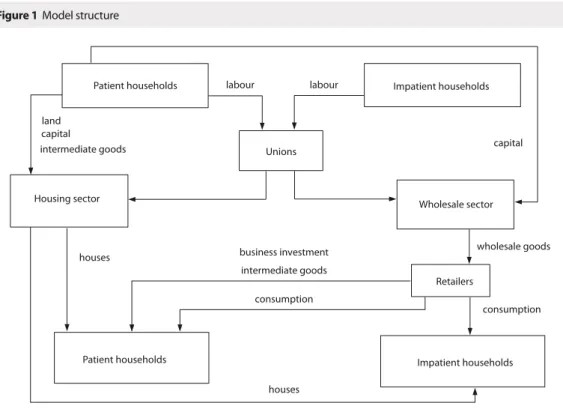
The model is borrowed from Iacoviello and Neri (2010) and ranks among medium-scale models. This model contains financial friction in the form of collateral constraint. This mechanism originates from Kiyotaki and Moore (1997), and was further elaborated in Iacoviello (2005), who used houses instead of land as collateral. Here, I describe only the main behavioural equations of the model; more detailed exposition is quoted in the online Appendix (available at the website of this journal, see the online version of the Statistika: Statistics and Economy Journal No. 4/2016 at: <http://www.czso.cz/statistika_journal>). Figure 1 provides basic orientation in the model structure.

2.1 Households

There are two types of households: patient (lenders) and impatient (borrowers). Patient households work, consume and accumulate housing. They also own capital and land, and supply funds to firms and to impatient households. Their utility function is:

(

)

⎠ ⎞ ⎟⎟

⎝ ⎛

+ + − + −

Γ +

+ + + −

∞

∑

η ξ ξ

η τ ε

β 1

1 1

, 1

, 1

0 = 0

1 ln ) ( ln )

( ct ht t

t t t t c t t C t

n n h

j c c z G

E , (1)

where ct,ht,nc,t,nh,t are consumption, housing, worked hours in the consumption sector and worked hours in the housing sector. ȕ is discount factor, İ is habit in consumption, ξ,η ≥ 0 are elasticities of substitution of

wor-Figure 1 Model structure

Patient households Impatient households

Unions

Wholesale sector Housing sector

Retailers

Impatient households Patient households

business investment labour labour

land capital

intermediate goods capital

intermediate goods

consumption houses

consumption wholesale goods

houses

ked hours in those two sectors. zt, jt and τt are shock to intertemporal preferences, housing preference shock

and shock to labor supply, all modelled as AR(1) processes. Gc is the growth rate of consumption along the balanced growth path. The scaling factor īc = (GCíİ)/(GCíȕİ*C) ensure that the marginal utility of

con-sumption is 1/c in the steady state.

Budged constraint (in real terms) for patient households is:

t wh t h t h t wc t c t c t t t l t t t b t h t k t c t X n w X n w b l p h q k k A k c , , , , , , , , , , , = + − + + + + +

(

)

δ 1 1

1 , , , , , 1 , , , , 1

1 − −

− − + + − + − ⎟ ⎟ ⎠ ⎞ ⎟ ⎟ ⎝ ⎛ − + + (2) 1 , , , 1 , , 1 1 , , ( ) ) ( ) (1 ) ( + ₋ + − ₋ + − − − − ₋

+ _{ht ht}

t k t c t c t t t h t t t l t

l a z k

A k z a Div h q l R

p δ φ .

Patient households choose consumption ct, capital in the consumption sector kc,t and housing sector kh,t, amount of intermediate goods kb,t (priced at pb,t) in the housing sector, housing ht (priced at qt), land lt, (priced

at pl,t), hours in consumption and housing sector nc,t and ns,t, capital utilization rates zc,t and zh,t and borrowing bt (loans if bt is negative) to maximize utility function (1) subject to the budget constraint (2). Ak,t is investment--specific technology shock which represents the marginal cost of producing capital used in the non-housing sector. Loans are set in nominal terms and yield a riskless nominal return R1. Real wages are denoted by wc,t

and wh,t, real rental rates by Rc,t and Rh,t and depreciation rates by įkc and įkh. The terms Xwc,t and Xwh,t

deno-te markup between the wage paid by the wholesale firm and wage paid to the households by labour unions.

ʌt = Pt/Pt–1 is inflation rate in the consumption sector, Divt are lump-sum profits from final goods firms and from labor unions, ϕt denotes total convex adjustment costs for capital and a(.) is the convex cost of setting capital utilization rate z.

Impatient households also consume, work and accumulate housing and their utility function is similar to that of patient households:4

(

)

∑

0 ( ' ( ')

1 ' ln ) ' ' ( ln )

( ct ht

t t t t t c t t C t n n h j c c z G

E . (3)

However, they do not accumulate capital and do not own finished-goods producing firms or land (their dividends come only from labor unions). Their budget constraint is as follows:

' ' ' ) (1 ' ' ' ' ' ' '

' 1 1

1 , , , , , , t t t t t h t t wh t h t h t wc t c t c t t t t Div b R h q X n w X n w b h q

c + ′− ′= + + − ₋ − − − +

π

δ . (4)

The impatient households are credit constrained and use their houses as collateral for loans. Their maxi-mum borrowing b't is given by the expected present value of their home times the loan-to-value (LTV) ratio:

⎟⎟ ⎠ ⎞ ⎟⎟ ⎝ ⎛ ≤ + + t t t t t t R h q mE

b_' 1 'π 1 _{. (5)}

4 _{The variables of impatient households are denoted with apostrophe (’), the meaning is the same as in case of patient}

This setting implies that variation in housing values shifts the borrowing constraint and thus affects their borrowing capacity and spending. There is also another channel for propagation of financial shocks into the real part of the economy: the debt-deflation effect. Debt is quoted in nominal terms,5 _{which is based on}

em-pirical grounds from low-inflation countries. The transmission mechanism then works as follows: positive demand shock increases the price of assets (housing), which increases the borrowing capacity of constrained households and allows them to spend more. The rise in prices reduces the real value of their debt obligations, which further increases value of their net worth. Borrowers have a higher propensity to spend than lenders, and thus net demand is positively affected. This mechanism, connected to housing wealth, works as an acce-lerator of demand shocks.

2.2 Firms

The production side of the model economy is divided into two sectors with different rates of technological progress. The firms hire labor and capital services and buy intermediate goods from households to produce wholesale goods Yt and new houses IHt. Their optimization problem is:

⎟⎟ ⎠ ⎞ ⎟⎟ ⎝ ⎛ + + + + −

+

∑

∑

∑

max , (6)

subject to the production functions:

(

)

(

)

t c t c c t c t c t c

t A n n z k

Y= α α μ ( , , 1)μ

1 1 , , , − − −

′ (7)

(

)

(

)

t b t b h t h t h l b h t h t h t h

t A n n z k k l

IH α α μ μ μ , , 1 μ μ, μ1

1 1 , , , ( ) = − − − − − −

′ . (8)

The wholesale good is produced using technology (7) with labor and capital inputs only. New houses IHt

are produced using technology (8) with labour, capital, land and the intermediate input kb . The terms Ac,t and

Ah,t denotes productivity in the non-housing and housing sector. Parameter Į measures labor income share of patient households.

2.3 Retailer and labour unions

There are nominal wage rigidities in both housing and non-housing sectors, and price rigidity in the retail sec-tor. The rigidities come from the existence of labour unions and retailers that have some market power and can influence setting of the wages and prices. The rigidities are modelled in Calvo (1983) style with partial indexa- tion to previous inflation. Optimization problem of the retailers results in hybrid New Keynesian Phillips curve:

t p t C t t t C t

t X X u

G E

G _{1 ,}

1 ln( / )

) )(1 (1 ) ln ln ( = ln

ln − _{− +} − − − − +

π π π π π θ θ β θ π ι π β π ι

π , (9)

where Xt is a markup over marginal cost, X is the steady state markup, șʌ is the fraction of firms that cannot

change the price every period and index it to previous inflation with elasticity Țʌ, and up,t is cost-push shock. Wage setting is analogous to price setting and the optimization problem of labor unions results in four wage Phillips curves (for each type of household in each production sector) that are similar to equation (9).

5 _{Expression R}

2.4 Monetary authority

Monetary authority sets the interest rate Rt according to (linearized) monetary rule with response to past interest rate, inflation and output growth:

t t R t t Y t R t R

t r R r r r y y rr u s

R = −1+(1− )[ππ + ( − −1)+ ]+ , − , (10)

where rr is the steady-state real interest rate, uR,t is monetary policy shock and st is shock to inflation target.

6

2.5 Market clearing and equilibrium condition

The non-housing sector produces consumption, business investment and intermediate goods. The housing sector produces new houses that are added to existing stock. The equilibrium conditions for product market and housing market are:

t t t b t h t k t c

t IK A IK k Y

C + ,/ ,+ , + , = −φ (11)

t t h

t H IH

H −(1−δ ) −1= , (12)

where Ct = c1 + ct' is aggregate consumption, Ht = h1 + ht' is aggregate stock of housing, and IKc,t = kc,t –

(1– įkc) kc,t–1 and IKh,t = kh,t – (1– įkh) kh,t–1 are two components of business investment.

2.6 Growth rates

The technological progress is allowed to be different across the sectors. The net growth rates of technology in housing sector (Ah,t), consumption goods sector (Ac,t) and investment goods sectors (Ak,t) are denoted as ȖA,H,  ȖA,C

and ȖA,K, respectively. Growth rates of the real variables along balanced growth path are then determined by:

AK c c AC IH q h IK

C G G

G γ μ μ γ − + + × 1 1 = =

= ₍₁₃₎

AK c AC c IK G γ μ γ − + + 1 1 1

= ₍₁₄₎

AH b l h AK c b h c AC b h IH

G γ μ μ μ γ

μ μ μ μ γ μ

μ (1 )

1 ) ( ) ( 1 = + − − − − + + + + (15) AH b l h AK c b h c AC b h q

G γ μ μ μ γ

μ μ μ μ γ μ

μ (1 )

1 ) (1 ) (1 1 = + − − − − − − + − − + . (16)

The trend growth rates of IKh,t, IKh,t/Ak,t and qtIHt are all equal to the trend growth rate of real consumption

Gc. Business investment GIK

c grows faster than consumption, as long as ȖA,K > 0 and the trend growth rate in real

house prices Gq offsets differences in the productivity growth between the consumption, Gc, and the housing sector GIH. The equilibrium model equations are linearized around balanced growth path before the estimation.

3 DATA AND ESTIMATION

The model is estimated using the data for the following model variables: consumption (Ct); residential investment (IHt); non-residential investment (IKt); real house prices (qt); inflation (ʌt); nominal interest rate (Rt); hours

worked and wage inflation in housing (NHt,Wht) and in the wholesale sector (NCt, WCt). I use quarterly data from the Czech Statistical Office and Czech National Bank databases for the period 1998:Q1–2013:Q2.

6 _{This shock is quite suitable for the Czech economy because during the period used for estimation the Czech National Bank}

The beginning of the sample period was determined by the availability of data on house prices, the ending of the sample was chosen with the aim to avoid complications with zero lower bound on interest rates. Time series for Ct, IHt, IKt and qt are in levels and are assumed trend stationary; the trend is estimated within

the model. Other time series are demeaned.7 _{As the data for the labour market in the housing sector (}

NHt,WHt)

might not be very reliable, measurement error for these two series was added.

Some of the model parameters are calibrated according to Iacoviello and Neri (2010) and data from national accounts.8 _{One of the calibrated parameters important for the analysis is loan-to-value ratio (LTV). Iacoviello}

and Neri (2010) calibrate LTV ratio to 0.85 for United States; the same value uses Walentin (2014) for Sweden while Christensen et al. (2009) calibrate it to 0.80. There is not much of empirical evidence about the value of this parameter for the Czech economy. Hloušek (2012) reports estimates of LTV ratios from DSGE model with both constrained households and entrepreneurs. His estimate for households is 0.79 and for entrepreneurs 0.51. Therefore, I set loan-to-value ratio to m = 0.75, taking into account that only constrained households are in the present model and also given the fact that the Czech mortgage market is less developed.

The rest of the model parameters were estimated using Bayesian techniques. The posterior distribution of the parameters was obtained using the Random Walk Chain Metropolis-Hastings algorithm. 1 000 000 draws in two chains with 500 000 replications each were generated, and 80% of replications were discarded so as to avoid influence of initial conditions and to calculate moments of posterior distribution from the draws of converged chains. The convergence was verified using MCMC diagnostics. All computations were carried out using Dynare toolbox (Adjemian et al., 2011).

4 ESTIMATION RESULTS

This section discusses the results of the estimation and examines the behaviour of the model. Table 1 shows prior means, standard deviations and posterior means together with 95% probability intervals for selected estimated deep parameters.9 _{The priors for the parameters are mostly set according to the Iacoviello and}

Ne-ri (2010) as their model exhibits some non-standard features (e.g. labour share of unconstraint households). Many other priors are quite standard in DSGE literature and are also commonly used in empirical studies for the Czech economy. Among those, only the prior mean for capital adjustment cost is set to a lower value of 5 (instead of 10) with reference to Slanicay (2013).

Parameters İ and İ represent habit formation in consumption, for patient and impatient households respecti-vely. The posterior mean of İ (0.42) is lower than the posterior mean of İ (0.52). On average, these numbers indicate quite a weak habit in consumption. Typical values obtained for the Czech economy are usually much higher, around 0.8 (see e.g. Slanicay, 2013). Capital adjustment cost is more important in the consumption goods sector; the mean of the parameter ϕk,c is much higher than the prior, and is higher than its counterpart in housing sector, parameter ϕk,h. The labour income share of constrained households (1±Į) was estimated at 0.28. This is slightly higher than the values found in empirical studies for the U.S. economy (0.21) or Sweden (0.18); see Iacoviello and Neri (2010) and Wallentin (2014).

A much higher estimate was obtained by Hloušek (2012) for the Czech economy (0.55) and Christensen et al. (2009) for Canada (0.38). However, these latter two papers used a different model structure. Estimated

7 _{The exception is nominal interest rate, which was detrended using the Hodrick-Prescott filter to obtain more easily}

interpretable data series. The time series for interest rate exhibits a visible decreasing trend. If it were to be demeaned, the interest rate would be below “equilibrium” level for almost the whole period from 2002–2013 (with a brief exception in 2008), which might not correspond to the view of the Czech National Bank at the time.

8 _{For full set of calibrated parameters, see online Appendix (available at the website of this journal, see the online version}

of the Statistika: Statistics and Economy Journal No. 4/2016 at: <http://www.czso.cz/statistika_journal>).

9 _{Results for other parameters and shocks are quoted in online Appendix (available at the website of this journal, see the}

values of Calvo parameters indicate that price and wage rigidities are almost equally important. This is in con-trast to empirical studies for the Czech economy revealing that wages were more rigid than prices, e.g. Hloušek and Vašíček (2007) or Andrle et al. (2009). Again, the different sector structures of the models could explain this phenomenon. Parameters in the Taylor rule show that the Czech National Bank pays great attention to interest rate smoothing, rR = 0.91, and to output growth, rY = 0.23. Even if the prior mean for rY was set to 0, which corresponds to strict inflation targeting, the information in the data was stronger. On the other hand, the posterior mean of the parameter of inflation rʌ= 1.34 is slightly lower than the mean of the prior, which is usually used in calibrated models.

The estimated parameters of technology growth rates (ȖV) can be used to compute trends of the model va-riables.10 _{The quarterly growth rates for consumption (}

GC), business investment (GIK), residential investment (GIH) and real house prices (GQ) are 0.46, 0.56, –0.28 and 0.74, respectively. The simple univariate trend cal-culated on data delivers the following slopes: 0.63, 0.78, –0.38 and 1.44. The model captures a relative relation between growth rates of the variables (GIH < GC < GIK < GQ) but fails to capture its magnitude. The model under-predicts growth in consumption, business investment and especially house prices. The reason for this is that the growth rates in the model are mutually connected because of the existence of a balanced growth path, but the growth rate in the data may be influenced by structural changes. To return to the model, the steep trend in house prices was mainly caused by negative technological progress in the housing sector.

Table 1 Prior and posterior distribution of structural parameters

Parameter Prior distribution Posterior distribution Density Mean S.D. Mean 2.5% 97.5% Habit formation

beta 0.50 0.08 0.42 0.33 0.52 beta 0.50 0.08 0.52 0.38 0.65 Capital adjustment cost

gamma 5.00 2.50 9.10 0.09 10.97 gamma 5.00 2.50 4.58 1.76 7.34 Labour income share

beta 0.65 0.05 0.72 0.65 0.80 Taylor rule

beta 0.75 0.10 0.91 0.89 0.93 normal 1.50 0.10 1.34 1.17 1.50 normal 0.00 0.10 0.23 0.09 0.37 Calvo parameters

beta 0.67 0.05 0.73 0.67 0.79 beta 0.67 0.05 0.76 0.72 0.80 beta 0.67 0.05 0.69 0.62 0.75 Technology growth rates

normal 0.50 1 0.41 0.37 0.46 normal 0.50 1 – 0.53 – 0.95 –0.09 normal 0.50 1 0.10 0.05 0.14

Source: Author’s calculations

The model fit on the data was evaluated by comparison of moments calculated from the data, and moments obtained from model simulations. One can argue that the empirical performance of the model is acceptable.11

To provide answers to the research questions various methods are used. Comparison of impulse responses for different model specifications is a key tool for examining the effects of housing collateral in the monetary policy transmission mechanism. The relationship between the housing sector and the rest of the economy is studied by variance decomposition of forecast errors, while historical shock decomposition is used to identify the shocks behind developments in real house prices.

4.1 Impulse Response Analysis

This section examines the behaviour of the model in reaction to shocks under different loan-to-value ratio assumptions. First, we will focus on an interpretation of impulse responses, and then we will carry out a quan-titative assessment of the transmission mechanism.

Figure 2 shows the reaction of the model variables to a monetary policy shock – the increase of nominal interest rate by one percentage point. The y-axis measures percentage deviation from the steady state; the re-action of the benchmark model is depicted by a solid line. A temporary increase in the nominal interest rate causes a drop in inflation by 2%; output decreases by as much as 9%, and house prices by 6%. Both types of investment decrease by roughly the same amount; however, residential investment returns faster. The dec-rease in investment is larger than that in output, which is, in turn, larger than in consumption. The reaction in consumption is hump-shaped, with a trough in the second period following the shock, and is long-lasting, with return after fifteen quarters. The consumption drop is driven primarily by the consumption of impatient (credit constrained) households: the fall in consumption is three times larger for impatient households than for patient households. This is for two reasons: first, collateral constraint becomes tighter because of the fall in house prices; second, there is the Fisher debt-deflation effect – an unexpected fall in inflation increases ex--post real interest rate, and thus results in an increased real debt burden. Therefore, wealth is transferred from borrowers to savers.

Figure 2 also shows the reaction of variables for other versions of the model. In all three specifications the estimated parameters are kept at their posterior means. In the benchmark model the loan-to-value ratio (para-meter ) is calibrated to 0.75, in the ”high collateral“ model it is 0.95, which means that constrained households are in a better position to obtain a loan; in the ”no collateral“ specification, the LTV is set to 0.0001, which means that houses are not collateralizable and impatient households are excluded from the financial market.

The reactions of the model variables for all three specifications are qualitatively identical but differ in mag-nitude, especially for consumption and output. Table 2 summarizes these findings. Each row shows the diffe-rence at trough of impulse responses for the corresponding variable between the specifications. The presence of collateral constraint (first row) does not produce much difference. However, an increase of LTV ratio from 0.75 to 0.95 (second row) causes a bigger drop in consumption by 4.5 and in output by 2.2 percentage points. On the other hand, the impact for inflation is quantitatively small (0.68 p.p.). Figure 3 shows the amplitude of the impulse responses in reaction to the LTV ratio (up to =0.95). This figure documents the fact that effect of LTV ratio is non-linear: a marginal increase at high values of LTV causes a much higher drop in all variables than a marginal increase at lower values of LTV. The results of this exercise lead to two conclusions: (i) mone-tary policy shocks are amplified when collateral effect is present and LTV ratio is high, and (ii) the impact for real variables such as consumption and output is much larger than the impact for inflation. Thus, restrictive monetary policy aimed at reducing inflation may result in large drops in real variables, when the LTV ratio is high. These results are in line with the findings of Walentin (2014) for the Swedish economy.

11 _{For details see the online Appendix (available at the website of this journal, see the online version of the}

Figure 4 shows a reaction to housing preference shocks that can be interpreted as an increase in demand for housing. This shock causes a very persistent increase in house prices. Since houses serve as collateral for constrained households, any raise in their price increases the households' borrowing capacity and thus their spending. Given the higher propensity of borrowers to consume, the overall impact on aggregate consump- tion is positive, even if consumption of unconstrained households (savers) falls. Both residential and business investment increase and so does output. Inflation also increases, and the central bank raises the interest rate in order to bring the economy back to steady state. Subsequently, the reaction of the economy to this shock is in line with the results of Walentin (2014) for the Swedish economy, where business investment also rises while it was found to decline for the U.S., as reported by Iacoviello and Neri (2010). Looking at other model specifications, the model with high LTV ratio (m = 0.95) produces qualitatively similar results but much larger deviations e.g. for consumption and inflation. On the other hand, when collateral constraint is switched off,

Figure 2 Impulse responses to monetary policy shock

0 5 10 15 20

−10 −5 0

consumption

0 5 10 15 20

−4 −2 0 2

consumption: patient HH

0 5 10 15 20

−40 −30 −20 −10 0

consumption: impatient HH

0 5 10 15 20

−20 −10 0 10

percentage deviation from steady stat

e

residential investment

0 5 10 15 20

−20 −10 0 10

business investment

0 5 10 15 20

−10 −5 0 5

house prices

0 5 10 15 20

−4 −2 0 2

inflation

quarters

0 5 10 15 20

−0.5 0 0.5 1

interest rate

quarters

0 5 10 15 20

−20 −10 0 10

output

quarters

benchmark high collateral no collateral

Source: Author’s construction

Table 2 Effect of collateral constraint on amplitude of impulse response to monetary policy shock (difference between IRFs at trough in percentage points)

Consumption Output Inflation IRF no collateral (m= 0) – IRF benchmark (m=0.75) 0.84 0.37 0.24

IRF benchmark (m=0.75) IRF high LTV (m=0.95) 4.45 2.20 0.68

the reaction of consumption, inflation and interest rate is the very opposite. However, this last model predic-tion contradicts the empirical evidence. Using the VAR model estimated on Czech data, Hloušek (2012) found that there is a positive co-movement of consumption and house price in response to house price shock.

Figure 4 Impulse responses to housing preference shock

Figure 3 Effect of different LTV on amplitude of impulse responses to monetary policy shock

0 0.2 0.4 0.6 0.8 1 −15

−10 −5 0

LTV

% deviation from

s.s

.

consumption

0 0.2 0.4 0.6 0.8 1 −15

−14 −13 −12 −11 −10 −9 −8 −7

LTV LTV

% deviation from

s.s

.

output

0 0.2 0.4 0.6 0.8 1 −4.0

−3.5 −3.0 −2.5 −2.0 −1.5 −1.0

LTV

% deviation from

s.s

.

inflation

benchmark LTV, m = 0.75

Source: Author’s construction

Source: Author’s construction

0 5 10 15 20

−1 0 1 2

consumption

0 5 10 15 20

−0.5 0 0.5

consumption: patient HH

0 5 10 15 20

−5 0 5 10

consumption: impatient HH

0 5 10 15 20

0 5 10

percentage deviation from steady stat

e

residential investment

0 5 10 15 20

−1 −0.5

0 0.5 1

business investment

0 5 10 15 20

0 1 2 3

house prices

0 5 10 15 20

−0.5 0 0.5

inflation

quarters

0 5 10 15 20

−0.1 −0.05

0 0.05 0.1

interest rate

quarters

0 5 10 15 20

0 0.5 1 1.5

output

quarters

Iacoviello (2005) obtained similar results for the United States. Therefore, the collateral effect is a necessary feature of the model for it to show a positive response in consumption to the house price shock, as is evident in the data.

Figure 5 shows the reaction of the variables to consumption goods technology shock. This shock results in cheaper production of consumption goods; therefore, inflation decreases, whilst consumption increases. Both types of investment increase, and thus output also increases. However, the drop in inflation is more significant than the rise in output and so the central bank lowers the interest rate. This shock is quite persistent and the deviation of the variables from steady state is thus long-lasting. There are only slight differences across the specifications. Collateral effect is not important here because this shock causes opposite reactions in house prices and inflation, and the amplification mechanism is dampened. The rise in house prices increases impa-tient households' borrowing capacity, while the decrease in inflation increases the real interest rate and causes a negative income effect for borrowers.

The collateral effect is important only for some kind of shocks: those that move house prices and inflation in the same direction. These are, specifically, monetary policy shock, housing demand shock, housing techno-logy shock and inflation target shock (the last two are not shown here). The increase of LTV to higher values against the benchmark amplifies short run responses in consumption, output or inflation, whose magnitudes vary according to the type of shock. These effects are quantitatively substantial and support a policy of setting maximum limits on LTV ratios, with the aim of reducing the volatility of the variables.

Figure 5 Impulse responses to consumption good technology shock

0 5 10 15 20

0 0.5 1 1.5

consumption

0 5 10 15 20

0 0.5 1 1.5

consumption: patient HH

0 5 10 15 20

0 1 2 3

consumption: impatient HH

0 5 10 15 20

0 0.5 1 1.5

percentage deviation from steady stat

e

residential investment

0 5 10 15 20

0 1 2 3

business investment

0 5 10 15 20

0 0.5 1 1.5

house prices

0 5 10 15 20

−0.4 −0.3 −0.2 −0.1 0

inflation

quarters

0 5 10 15 20

−0.06 −0.04 −0.02

0

interest rate

quarters

0 5 10 15 20

0 0.5 1 1.5 2

output

quarters benchmark high collateral no collateral

Figure 6 Variance decomposition

4.2 Variance Decomposition

Figure 6 shows a conditional variance of the model variables explained by each shock for a one-, eight- and twenty-quarter forecast horizon, and an unconditional forecast error variance decomposition. There is an in-teresting pattern to be observed: monetary policy shock, cost-push shocks and inflation target shocks are quite important in the short term, not only for the nominal variables but also the real variables. However, their influence on the real variables fades over time. The opposite is true for technology shocks, whose influence increases with time. Housing preference shocks are more or less stable in explaining the variance of residential investment and real house prices.

The last columns of the Figure 6 show an unconditional variance decomposition and deserves bigger attention. Productivity shocks in the non-housing sector for consumption goods explain most of the volatility in consumption, business investment and output. On the other hand, investment-specific technology shocks are unimportant even for business investment. Housing technology and preference shocks are important for the behaviour of residential investment (IH) and house prices (q), while the latter is more significant in the shorter term (compare with the previous part). Inflation target shocks are mainly responsible for variance in interest rate (R) and together with cost-push shocks also for variance in inflation (ʌ). Labour supply shocks and intertemporal shocks are relatively unimportant.

The central objective of this paper is to assess the relationship between the housing market and the rest of the economy. One can see that there is a large degree of disconnection. Both housing market shocks (technology and preferences) explain in sum 96% of variance in housing investment and 90% of variance in housing prices.12 _{As regards non-housing shocks, only consumption good technology shocks play some role}

in the variance in housing prices. The opposite also holds: housing market shocks explain about ten percent of output variance (mostly through housing investment) but almost zero variance in inflation. Therefore spill-overs of housing specific shocks into the broader macroeconomy can be considered negligible. Poten- tial problems in the housing sector do not therefore represent any threat for the economy in this benchmark setting.

The effects of LTV ratio on the monetary transmission mechanism that were analysed by impulse respon-ses in the previous section can be further illustrated by looking at the unconditional forecast error variance decomposition. Table 3 shows the variance of consumption, output and inflation accounted for by monetary policy shock for different values of LTV ratio. When the LTV is increased from 0.75 to 0.95, monetary policy shocks have a larger effect, especially on consumption (more than twofold) followed by inflation and output (by 32%). When the collateral effect is switched off (m = 0), monetary policy shocks explain a smaller fraction of the variability, but the difference from the benchmark is intangible. These results repeatedly confirm the fact that increasing LTV amplifies the ability of monetary policy to influence consumption, output and in-flation, with its largest effect being on consumption. Contrary to the results obtained from impulse responses,

Table 3 Unconditional variance decomposition: effect of monetary policy shock (in %)

Consumption Output Inflation High LTV (m=0.95) 8.4 7.5 15.6 Benchmark (m=0.75) 3.8 5.7 11.8 No collateral (m= 0) 2.8 5.5 9.6

Source: Author’s calculations

12 _{See Table 5 in the online Appendix for exact numbers (available at the website of this journal, see the online version}

the impact of higher LTV for output and inflation here is quantitatively similar. This is due to the fact that in IRF analysis we considered the very short term impacts, while the forecast error variance decomposition is calculated for the long-term and, as was documented in Figure 6, the effect of monetary policy shock for output strongly decreases with time.

Finally, Table 4 shows the effect of different values of LTV ratio on the variance decomposition of selected variables following housing preference shock. Again, high values of LTV amplify the impacts of the shock, especially for consumption and inflation. In this case, the spill-overs to the broader macroeconomy can be considered nontrivial, and may justify setting caps on the loan-to-value ratio. Regarding housing techno- logy shock (not shown here), the impacts on macroeconomic variables increase only slightly with increasing LTV ratio.

4.3 Historical Shock Decomposition

While variance decomposition relates to forecast error of exogenous shocks to particular variables, historical shock decomposition performs an error decomposition on historical data. Figure 7 depicts the historical de-composition of real house prices into shocks during the estimated period. It shows that housing preference shocks became more significant from the end of 2001; from this moment onwards, they were the main deter-minant of rising house prices. The same shocks were responsible for the subsequent house price decline du-ring and after the crisis. Housing technology shocks also contributed to the development of house prices, but in a more stable way. Consumption goods technology shocks also increased their influence on the behaviour of house prices, mainly from 2002. After the peak in 2008, these non-housing technology shocks diminished, just as house prices declined. This analysis shows that both the demand and supply shocks played important roles; however, demand shocks were overall responsible for the fluctuation of house prices.

Table 4 Unconditional variance decomposition: effect of housing preference shock (in %)

Consumption Output Inflation High LTV (m=0.95) 8.6 5.7 4.7 Benchmark (m=0.75) 0.1 2.5 0.1 No collateral (m= 0) 0.6 2.7 0.6

Source: Author’s calculations

CONCLUSION

This paper presents the results of an estimation of a medium-scale DSGE model with housing sector using Czech data. The answer to the research question, regarding a possible connection between the housing sector and the rest of the economy, is rather complex. According to the forecast error variance decomposition, there is no significant link between these sectors. Housing sector shocks do not transfer to the broader economy, and only consumption good technology shocks explain some of the variability in real house prices.

If we look at the historical behaviour of house prices, shocks to housing preferences were their main driving force, especially during the turbulent past ten years. Technology shocks in the consumption goods sector and housing sector also contributed to raising house prices, but in a more stable manner.

Source: Author’s construction

per

ce

ntage deviation fr

om st

eady-stat

e

70

60

50

40

30

20

10

0

-10

-20

1998 2000 2002 2004 2006 2008 2010 2012

13 _{Iacoviello (2014) presents a model with borrower defaults and the propagation of financial shocks to the real economy}

through the banking system.

is not so distinctive. Moreover, the value of LTV amplifies these responses in a non-linear way. A marginal increase in LTV at high values of this variable causes a larger impact, especially for consumption and output, than a marginal increase at lower values of LTV.

Similar amplification is also observed for housing preference shock and its impacts on macroeconomic variables. High values of LTV ratio magnify the impacts of this shock, especially for consumption and in-flation. This outcome partly modifies the previous results that suggested disconnection between the sectors, instead indicating potential threats from the housing sector. There is also another potential cost connected with high LTV, which was not considered in the model, and that is that high LTV increases the probability of households defaulting on their loans, which can have impacts on the stability of the financial system and con-sequently on the whole macroeconomy.13 _{These results should be taken into consideration in the formation of}

macroeconomic policy that will set limits on loan-to-value ratio. Such a practice has already been introduced in Sweden where LTV is limited to a maximum 85% (Swedish Financial Supervisory Authority, 2010). The aim of this policy was to decrease risk in the credit market that stems from the inability of heavily indebted borrowers to repay their debts.

The impacts of LTV ratio were illustrated in this paper in reaction to disinflationary (restrictive) monetary policy, which caused welfare losses in terms of consumption or output. As the model assumes symmetry, we would obtain equivalent but opposite effects for the case of a decrease in interest rate by the monetary autho-rity. However, we might see asymmetric behaviour in consumption and output: a lower interest rate increases house prices and housing wealth, but the collateral constraint does not need to be binding. Credit constrained households become unconstrained following such a move, and change their consumption only a little compared with the case of restrictive monetary policy and low house prices. Another related issue is the zero lower bound on interest rate, which prevents the central bank from decreasing the interest rate, and may also contribute to the asymmetric behaviour of consumption and output. Guerrieri and Iacoviello (2014) explore these asymme-tries, but focus mainly on house price shocks. This could therefore be an appropriate topic for further research.

ACKNOWLEDGMENT

This paper is supported by specific research project No. MUNI/A/1049/2015 at Masaryk University. I would like to thank to two anonymous referees for their valuable comments that improved the paper. Next, I thank Jan Čapek for his technical help, and Martin Slanicay, Daniel Němec, Jan Brůha and Martin Fukač for offering a number of useful comments.

References

ADJEMIAN, S., BASTANI, H., JUILLARD, M., MIHOUBI, F., PERENDIA, G., RATTO, M., VILLEMOT S. Dynare: Reference Manual, Version 4. Dynare Working Papers, 1, Cepremap, 2011.

ANDRLE, M., HLÉDIK, T., KAMENÍK, O., VLČEK, J. Implementing the New Structural Model of the Czech National Bank. Czech National Bank: WP series, 2, 2009.

AOKI, K., PROUDMAN, J., VLIEGHEY, G. House prices, consumption, and monetary policy: a financial accelerator approach. Bank of England: WP series, 169, 2002.

BRŮHA, J. HLAVÁČEK, M., KOMÁREK L. Impacts of housing prices on the financial position of households. In: CNB Financial Stability Report2012/2013, Czech National Bank, Research Department: Occasional Publications – Chapters in Edited Volumes, 2013, pp. 120–127.

CALVO, G. Staggered prices in a utility-maximizing framework. Journal of Monetary Economics 12, 1983, pp. 383–398. CZECH NATIONAL BANK. Zpráva o finanční stabilitě 2013/2014 [online]. Prague: Czech National Bank, 2014. Available

at: <http://www.cnb.cz/cs/financni_stabilita/zpravy_fs/fs_2013-2014/index.html#1>.

ÉGERT, B., MIHALJEK, D. Determinants of House Prices in Central and Eastern Europe. Czech National Bank: WP series 1, 2008.

GALATI, G., MOESSNER, R. Macroprudential policy – a literature review. BIS Working Papers, No. 337, 2011.

GALÍ, J. Monetary Policy, Inflation, and the Business Cycle: An Introduction to the New Keynesian Framework. Princeton: Princeton University Press, 2008.

GUERRIERI, L., IACOVIELLO, M. Collateral Constraints and Macroeconomic Asymmetries [online]. Working paper, 2014 (April). Available at: <https://www2.bc.edu/matteo-iacoviello/research_files/ASYMMETRIES_PAPER.pdf>.

HLAVÁČEK, M., KOMÁREK, L. Regional Analysis of Housing Price Bubbles and Their Determinants in the Czech Republic. Czech Journal of Economics and Finance, Vol. 61, No. 1, 2011, pp. 67–91.

HLOUŠEK, M., VAŠÍČEK, O. Sensitivity Analysis of DSGE Model of Open Economy with Nominal Rigidities. In: Mathematical Methods in Economics, Liberec: Technical University of Liberec, 2008, pp. 192–197.

HLOUŠEK, M. DSGE model with collateral constraint: estimation on Czech data. In: RAMÍK, J., STAVÁREK, D. Proceedings of 30th International Conference Mathematical Methods in Economics, Karviná: Silesian University, School of Business Administration, 2012, pp. 296–301.

HLOUŠEK, M. DSGE model with housing sector: application to the Czech economy. In: Proceedings of 31st International Conference Mathematical Methods in Economics, Jihlava: College of Polytechnics Jihlava, 2013. pp 261–266.

CHRISTENSEN, I., CORRIGAN, P., MENDICINO, C., NISHIYAMA, S. Consumption, Housing Collateral, and the Canadian Business Cycle. Bank of Canada, Working paper 26, 2009.

IACOVIELLO, M. House Prices, Borrowing Constraints, and Monetary Policy in the Business Cycle. American Economic Review, Vol. 95, No. 3, 2005, pp. 739–764.

IACOVIELLO, M. Financial Business Cycles [online]. Working paper, 2014 (January). Available at: <https://www2.bc.edu/ matteo-iacoviello/research_files/FBC.pdf>.

IACOVIELLO, M., NERI, S. Housing Market Spillovers: Evidence from an Estimated DSGE Model. American Economic Journal: Macroeconomics, Vol. 2, No. 2, 2010, pp. 125–164.

KIYOTAKI, N., MOORE, J. Credit Cycles. The Journal of Political Economy, Vol. 105, No. 2, 1997, pp. 211–248.

MANDEL, M., TOMŠÍK, V. Monetary Policy Efficiency in Conditions of Excess Liquidity Withdrawal. Prague Economic Papers, No. 1, 2014.

POSEDEL, P., VÍZEK, M. Are House Prices Characterized by Threshold Effects? Evidence from Developed and Post-Transition Countries. Czech Journal of Economics and Finance, Vol. 61, No. 6, 2011, pp. 584–600.

ROEGER, W., IN’T VELD, J. Fiscal Policy with Credit Constrained Households. European Commission: European Economy – Economic Papers 357, 2009.

RYŠÁNEK, J., TONNER, J., TVRZ, S., VAŠÍČEK, O. Monetary policy implications of financial frictions in the Czech Republic. Czech Journal of Economics and Finance, Prague: UK FSV, Vol. 62, No. 5, 2012, pp. 413–429.

SLANICAY, M. Business Cycle Synchronization through the Lens of a DSGE Model. Czech Journal of Economics and Finance, Vol. 63, No. 2, 2013, pp. 180–196.

SWEDISH FINANCIAL SUPERVISORY AUTHORITY (FINANSINSPEKTIONEN). Limitation on loan-to-value ratios for mortgages on residential property [online]. Press release, 2014. Available at: <http://www.fi.se/Folder-EN/Startpage/ Supervision/Miscellaneous/Listan/Limitation-on-loan-to-value-ratios-for-mortgages-on-residential-property/>. TONNER, J., BRŮHA, J. Czech Housing Market through Lens of a DSGE model with Collateral Constrained Households.

WALENTIN, K. Housing collateral and the monetary transmission mechanism. The Scandinavian Journal of Economics, Vol. 116, Iss. 3, 2014 (July), pp. 635–668. DOI: 10.1111/sjoe.12064.

WALSH, C. E. Monetary Theory and Policy. 3rd _{Ed. Cambridge: MIT Press, 2010.}

WOODFORD, M. Interest and Prices: Foundations of a Theory of Monetary Policy. Princeton: Princeton University Press. 2003. ZAMRAZILOVÁ, E. Monetary Policy: Short-Term Stabilization versus Long-Term Risks. Politická ekonomie, No. 1, 2014. ZEMČÍK, P. Is There a Real Estate Bubble in the Czech Republic? Czech Journal of Economics and Finance, Vol. 61, No. 1,

2011, pp. 67–91.

APPENDIX