www.atmos-chem-phys.net/16/2155/2016/ doi:10.5194/acp-16-2155-2016
© Author(s) 2016. CC Attribution 3.0 License.
On the vertical distribution of smoke in the Amazonian atmosphere
during the dry season
Franco Marenco1, Ben Johnson2, Justin M. Langridge3, Jane Mulcahy4, Angela Benedetti5, Samuel Remy6, Luke Jones5, Kate Szpek3, Jim Haywood2,7, Karla Longo8, and Paulo Artaxo9
1Satellite Applications, Met Office, Exeter, UK
2Earth System and Mitigation Science, Met Office Hadley Centre, Exeter, UK 3Observational Based Research, Met Office, Exeter, UK
4Earth System Core Development Group, Met Office Hadley Centre, Exeter, UK 5European Centre for Medium-range Weather Forecasts, Reading, UK
6Laboratoire de Météorologie Dynamique, UPMC/CNRS, Paris, France
7College of Engineering, Maths and Physical Sciences, University of Exeter, Exeter, UK 8Instituto Nacional de Pesquisas Espaciais, São José dos Campos, Brazil
9Institute of Physics, University of São Paulo, São Paulo, Brazil
Correspondence to:Franco Marenco ([email protected])
Received: 23 October 2015 – Published in Atmos. Chem. Phys. Discuss.: 12 November 2015 Revised: 28 January 2016 – Accepted: 7 February 2016 – Published: 25 February 2016
Abstract. Lidar observations of smoke aerosols have been analysed from six flights of the Facility for Airborne Atmo-spheric Measurements BAe-146 research aircraft over Brazil during the biomass burning season (September 2012). A large aerosol optical depth (AOD) was observed, typically ranging 0.4–0.9, along with a typical aerosol extinction co-efficient of 100–400 Mm−1. The data highlight the
persis-tent and widespread nature of the Amazonian haze, which had a consistent vertical structure, observed over a large dis-tance (∼2200 km) during a period of 14 days. Aerosols were
found near the surface; but the larger aerosol load was typi-cally found in elevated layers that extended from 1–1.5 to 4– 6 km. The measurements have been compared to model pre-dictions with the Met Office Unified Model (MetUM) and the ECMWF-MACC model. The MetUM generally reproduced the vertical structure of the Amazonian haze observed with the lidar. The ECMWF-MACC model was also able to re-produce the general features of smoke plumes albeit with a small overestimation of the AOD. The models did not always capture localised features such as (i) smoke plumes originat-ing from individual fires, and (ii) aerosols in the vicinity of clouds. In both these circumstances, peak extinction coeffi-cients of the order of 1000–1500 Mm−1and AODs as large
as 1–1.8 were encountered, but these features were either
un-derestimated or not captured in the model predictions. Smoke injection heights derived from the Global Fire Assimilation System (GFAS) for the region are compatible with the gen-eral height of the aerosol layers.
1 Introduction
Biomass burning is the second largest source of anthro-pogenic aerosols globally (Stocker et al., 2013), and South America features as one of the major source regions. In Southern Amazonia, fire is often used for deforestation and for the preparation of agricultural fields and pasture (Brito et al., 2014). The dry season spans from July to October every year, and controls the timing of the intensive burning of the vegetation. Intense precipitation can still occur in this season, due to the increase of convective available potential energy (CAPE) and moisture, associated with the Monsoon circu-lation (Gonçalves et al., 2015). The rate of biomass burning in the Brazilian rainforest varies from year to year and is af-fected by meteorological conditions as well as social factors (Kaufman et al., 1998).
climate (Sena et al., 2013; Rizzo et al., 2013). Episodes of poor air quality and low visibility are frequent, and the aerosol loadings affect the radiation budget and the cloud mi-crophysics (Kaufman et al., 1998). Moreover, the radiative balance of the region is also affected by changes in the sur-face albedo caused by burning of the vegetation. The latter has an impact well beyond the burning season, as it affects the regional surface energy budget all year round, and has an impact on convection, cloud formation and precipitation (Sena et al., 2013).
The modified ratio of direct to diffuse radiation, and the changes in meteorology, in turn will affect the photosynthet-ically active radiation flux and the carbon cycle (Mercado et al., 2009). Given that Southern Amazonia is the Earth’s largest hydrological basin, the largest carbon sink, and the largest tropical rainforest, the changes in the regional at-mosphere and biosphere introduced by biomass burning can have a relevant impact at the global scale. A detailed review of the literature on biomass burning emissions can be found in Koppmann et al. (2005) and Reid et al. (2005b, a).
The large amount of heat released by forest fires can gen-erate strong updrafts and deep convection in their vicinity, rapidly transporting aerosols to upper layers (Freitas et al., 2007; Labonne et al., 2007; Sofiev et al., 2012), followed by long-range transport (Kaufman et al., 1998). Aerosols can be transported for thousands of kilometres, and as they travel they are modified through ageing processes (Hobbs et al., 1997; Kaufman et al., 1998; Fiebig et al., 2003; Vakkari et al., 2014). The composition of biomass burning aerosols is dom-inated by fine carbonaceous particles (organics and black carbon; see Brito et al., 2014), and in the first 2 hours after emission aerosol scattering can increase up to a factor of six due to photochemistry and secondary particle formation; this is particularly the case for smouldering fires (Vakkari et al., 2014). Particle hygroscopicity and the concentration of CCN are also enhanced during ageing (Abel et al., 2003).
Further downwind, these aerosols continue to exert an im-pact on cloud formation, convection, and precipitation pat-terns (Andreae et al., 2004; Koren et al., 2008). Gonçalves et al. (2015) indicates two opposite mechanisms by which biomass burning aerosols affect clouds and precipitation: (i) in a stable atmosphere, for a given liquid water content the formation of a larger number of smaller cloud droplet induces warm rain suppression; and (ii) in an unstable at-mosphere, the aerosols enhance precipitation and favour the formation of larger and long-lived cells (convective cloud in-vigoration). Moreover, Seifert et al. (2015) have observed an increased ice formation efficiency for clouds in the dry sea-son, and a coincidence with the seasonal aerosol cycle.
Knowledge of the vertical structure of the Southern Ama-zonia smoke layer is key to understanding and assessing the aerosol–cloud interactions (Baars et al., 2012). Textor et al. (2006) showed that there are significant uncertainties in the vertical distribution in global models, whereas this infor-mation is critical in assessing the magnitude and even the
sign of the direct radiative forcing. Of particular interest are the distribution of lofted layers (Mattis et al., 2003; Müller et al., 2005; Baars et al., 2012) and the identification of com-plex scenes involving both aerosols and clouds (Chand et al., 2008).
The South AMerican Biomass Burning Analysis (SAMBBA) campaign was an intensive field project (September–October 2012), aimed at collecting information on the atmosphere of the Amazon basin during the dry season and the transition into the wet season (Angelo, 2012). One important focus has been the impact of biomass burning aerosol on the radiation budget, and its feedback on the dynamics and hydrological cycle, including the influence on numerical weather predictions, climate, and air quality. The partnership involved mainly scientists from Brazil (National Institute for Space Research, INPE, and University of Sao Paulo) and from the United Kingdom (the Met Office and the Natural Environment Research Council).
2 Research flights
During SAMBBA, the Facility for Airborne Atmospheric Measurements (FAAM) research aircraft was based in Porto Velho, Brazil (8◦44′S 63◦54′W), and 20 research flights were carried out between 14 September and 3 October 2012, totalling 65 h of atmospheric research flying. Porto Velho lies in the state of Rhondonia, where biomass burning for deforestation and agriculture is prevalent, and a large de-forested area is evident. The flights sampled a wide range of conditions, from very low concentrations of gas phase and aerosol species over the pristine Amazonia rainforest, through to major fire plumes emitting very large amounts of pollutants. Some of the flights were coordinated with satellite overpasses, which allowed combining aircraft measurements with spaceborne remote sensing (see, e.g., Marenco et al., 2014).
The aircraft was equipped with several probes, able to sample the atmosphere using both in situ and remote-sensing techniques. Each research flight was planned around one of the following goals: (a) in situ characterisation of fresh plumes (FP), achieved by flying at low level in the immediate vicinity of a fire and sampling the aerosols, trace gases and thermodynamic structure; (b) radiative closure (RC) studies, achieved with a series of stacked aircraft runs and profiles above a limited area, in order to tie together the information derived by remote sensing and the in situ probes; and (c) sur-vey flights (SF) at high altitude, where the properties of the atmosphere are mainly sampled with remote-sensing tech-niques. Besides Porto Velho (PV), the airports in Rio Branco (450 km WSW of PV), Manaus (760 km NE of PV) and Pal-mas (1700 km E of PV) were also used.
low-mid tropospheric circulation is halted by the Andes. In this season, the north-western part of the basin is charterised by the development of deep convective events ac-companied by brief but intense precipitation, whereas the Southern and Eastern parts are typically dry. The season in 2012, however, differed somewhat from the climatology. A Northwesterly circulation on the Southwestern part of the basin dispersed the aerosols, and as a result only a moderate aerosol optical depth (AOD) was observed. Moreover, con-vective precipitation spread further East than usual during the second half of September.
Nevertheless, burning activity continued through the ma-jority of the campaign period, and significant aerosol load-ing was found durload-ing most of the flights. In the majority of cases, a variety of measurements confirmed that the aerosols can be ascribed to smoke originated from forest fires. A gen-eral feature throughout the campaign was the persistence of aerosols above the boundary layer, with plumes up to alti-tudes of 4–6 km, presumably caused by deep convection and lifting. In situ observations with wing-mounted optical par-ticle counters (PCASP and CDP; see, e.g., Liu et al., 1992; Lance et al., 2010; Rosenberg et al., 2012; Ryder et al., 2013) showed a predominance of fine mode particles at all levels (elevated and near-surface). Moreover, measurements with the on-board AL 5002 VUV Fast Fluorescence CO Analyser (Gerbig et al., 1996, 1999; Palmer et al., 2013) showed high carbon monoxide concentrations.
The present study focuses on the results from the airborne lidar during the high-altitude portions of six selected flights, between 16 and 29 September (see Table 1 and Fig. 1). The criterion for selecting the flights has been the availability of sufficiently extended high-altitude and cloud-free sections, so that the aerosol extinction vertical profile could be esti-mated from the lidar. The six flights span the region between 8.5–12◦N and 46–68◦W, covering a distance of∼2200 km extending along an East–West axis across the Brazilian Ama-zon basin, at an approximate mean latitude of 10◦S.
3 Measurements
Observations of atmospheric aerosols have been acquired with the ALS-450 elastic backscattering lidar mounted on the FAAM research aircraft. This is an instrument manufactured by Leosphere; it is operated at a wavelength of 355 nm; and it is mounted in a nadir-looking geometry (Marenco et al., 2011). The system specifications are summarised in Marenco et al. (2014) and a more detailed description of the instrument can be found in Lolli et al. (2011) and Chazette et al. (2012). Lidar signals were acquired with an integration time of 2 s and a vertical resolution of 1.5 m. The analogue and photon counting signals are merged at pre-processing by normali-sation in an overlap area chosen based on photon-counting thresholds. Cloud signal in the vertical profiles was detected as a “large spike”, and the thresholds given in Allen et al.
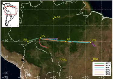
Figure 1.Ground tracks for the six research flights listed in Table 1. The location of the valid lidar profiles used for the computation of aerosol extinction is highlighted as follows: grey, profiles that pass our quality control test; blue, remaining profiles. The follow-ing locations are also shown: Porto Velho (PV), Rio Branco (RB), Alta Floresta (AF), Palmas (Pal), Manaus (Man), Cuiabà (Cui), and Brasilia (Bra).
(2014) were applied to determine their top height at 2 s reso-lution.
In order to determine the aerosol properties, further inte-gration and vertical smoothing have been applied during data processing, to reduce shot noise: the aerosol data presented here therefore have a vertical resolution of 45 m and an inte-gration time of 1 min. This inteinte-gration time corresponds to a 9±2 km footprint, at typical aircraft speeds.
A first data selection was done as follows: all lidar signals acquired when the aircraft was flying at an altitude lower than 4 km have been omitted, and data have been discarded if the lidar was pointing at more than 10◦off the vertical (due to the aircraft turning). Lidar signals within 300 m of the air-craft have been discarded, due to incomplete overlap between the emitter and the receiver field-of-view, and at the far end profiles have been truncated to remove the surface spike and any data beyond it. As a general rule, a vertical profile where a cloud was detected has either been omitted completely, or has been omitted in the portion between the surface and the cloud top. However, in a small number of cases where the cloud optical depth has been considered sufficiently small, so as to not affect the derivation of aerosol properties, data below a cloud have been kept but the cloud layer itself has been rejected.
(extinction-to-Table 1.Research flights considered in this article. Time is UTC.
Flight Date Takeoff Landing Latitude Longitude Type∗
B733 16 Sep Rio Branco, 13:51 Porto Velho, 14:45 8.9–9.8◦S 64.5–67.6◦W brief SF
B734 18 Sep Porto Velho, 12:05 Porto Velho, 16:01 8.9–11.9◦S 61.6–64.4◦W RC
B741 26 Sep Porto Velho, 12:53 Palmas, 16:08 8.8–10.2◦S 48.7–63.9◦W SF
B742 27 Sep Palmas, 12:52 Palmas, 16:17 10.2–11.5◦S 46.8–48.1◦W FP
B743 27 Sep Palmas, 18:08 Porto Velho, 21:34 9.0–10.2◦S 48.4–63.6◦W SF
B746 29 Sep Porto Velho, 12:54 Porto Velho, 16:38 8.7–9.4◦S 58.2–63.7◦W FP+SF
∗Flight type: FP: fresh plume sampling, mainly in situ; RC: radiative closure, combining in situ and remote sensing; SF: high-altitude survey flight.
backscatter ratio), and subsequently to process the data set to determine the extinction coefficient. The method detailed in Marenco (2013) is at the basis of this processing, and it is based on setting the reference within the aerosol layer, rather than on a Rayleigh-scattering portion of the atmosphere. The slope method is used for a first estimate of the extinction co-efficient at the reference, based on the lidar measurements themselves. As illustrated in that paper, in this geometry and at this wavelength the forward solution to the lidar equation is unstable and cannot be used when the aerosol layers are deep and their extinction is large; hence the need for using this method. Marenco et al. (2014) illustrates the application of this method in comparison with CALIPSO retrievals and to constrained retrievals using AERONET.
3.1 Lidar ratio
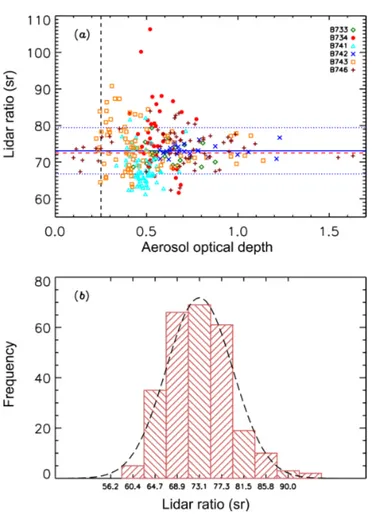
An initial subset of the lidar profiles has been selected, where the signature of Rayleigh scattering has been clearly identi-fied above the aerosol layers. This circumstance permits it-eration using the method described in Marenco (2013) by varying the lidar ratio (assumed constant with height), until a good match to the overlying Rayleigh scattering layer is reached: in this way, the lidar ratio itself can be estimated. Out of these lidar profiles, 270 indicate at least a moderate aerosol load (AOD>0.25), and they have been kept to com-pute a distribution: results are displayed in Fig. 2b. The data set follows a Gaussian distribution, and is characterised by a mean and standard deviation of 73.1 and 6.3 sr, respectively. Moreover, Fig. 2a shows that the distribution is not signifi-cantly affected by how we choose the acceptance threshold (AOD>0.25). The lidar ratio determined in this way is not substantially affected by the choice of the lower reference extinction, and is instead mainly affected by the higher lay-ers, where the transition between a large extinction coeffi-cient and a molecular layer is encountered. This estimate of the lidar ratio for biomass burning aerosols is in agreement with the findings reported in Omar et al. (2009), Baars et al. (2012), Groß et al. (2012), and Lopes et al. (2013).
The lidar ratio so determined, 73±6 sr, has been compared
to Mie scattering computations. Figure 3a displays the cam-paign mean particle size-distribution (PSD) determined with
Figure 2. (a)Lidar ratio and AOD, determined for each lidar pro-file (see text). The data points are colour-coded with the flight num-ber. The horizontal blue solid line indicates the mean, the blue dot-ted lines indicate one standard deviation from the mean, and the dashed red line indicates the median. The vertical dashed line in-dicates the threshold (AOD>0.25) that has been applied to the
data set.(b)Histogram of lidar ratio determinations, for 270 profiles
with AOD>0.25. Mean: 73.1 sr, standard deviation: 6.3 sr, median:
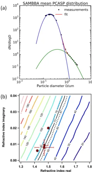
Figure 3. (a)SAMBBA campaign mean particle size-distribution,
determined with the wing-mounted PCASP optical particle counter (black dots). The fit with a bimodal lognormal is also shown; the parameters of the two lognormals are as follows: accumulation mode:Dp=0.184 µm,σ=1.47, andNt=868.5. Coarse mode: Dp=0.387 µm,σ=2.13, andNt=2.16.(b)Contours of the lidar
ratio computed for the campaign mean particle size-distribution, by varying the refractive index. The black solid and dotted lines indi-cate the mean and standard deviation of the lidar ratio determined by lidar (73±6 sr). The red dots show estimates of the Amazonian
biomass burning aerosol refractive index taken from the literature: (a) 1.5−0.02i(Reid and Hobbs, 1998); (b) 1.42−0.006i(Guyon
et al., 2003); (c)(1.47±0.07)−(0.008±0.005)i(Rizzo et al., 2013);
(d)(1.47±0.03)−(0.0093±0.003)i(Dubovik et al., 2002).
the PCASP, and its fit using two lognormals, each of which is in the form
n(D)=√ Nt
2πlnσ
e−
1 2
lnD/Dp lnσ
2
D , (1)
whereDis diameter, andDp,σ, andNt are three fitted pa-rameters (Johnson et al., 2016). We have computed the lidar ratio for this size-distribution and for a range of refractive
indices; see Fig. 3b. The resulting lidar ratio is highly depen-dent on the real and imaginary parts; refractive index esti-mates from the literature are also shown in the figure. The lidar derivation of 73±6 sr is compatible, for instance, with refractive indices from Rizzo et al. (2013) and Dubovik et al. (2002). Note that the estimates computed with refractive in-dices from Reid and Hobbs (1998) and Guyon et al. (2003) also do not fall too far off.
3.2 Estimate of the aerosol extinction coefficient
Following the result of the first iteration on the lidar data, a lidar ratio of 73 sr has been adopted for the full data set, and a second iteration with the method introduced in Marenco (2013) has been applied to determine the aerosol extinc-tion coefficient for all the 334 profiles. This method (slope-Fernald method) is a variant of the (slope-Fernald–Klett method (Fernald, 1984; Klett, 1985), where the reference is taken within an aerosol layer: this permits using the stable (inward) solution to the lidar equation in the unfavourable geometry represented by a nadir-looking lidar. Note that this choice is necessary if, as found during this campaign, no aerosol-free region below the aerosol layers is available. Figure 4 shows typical resulting estimates of the aerosol extinction coefficient, for a subset of the vertical profiles (this selec-tion is purely illustrative in purpose). For each profile, an estimate of the uncertainty that results from the retrieval as-sumptions has been computed, by repeating the derivation after having varied the lidar ratio by±6 sr (this being the
un-certainty adopted above), and after having varied the extinc-tion value at the reference by±50 % (1σ statistical errors). The latter value reflects the large uncertainty that arises from the Marenco (2013) method, since reference is taken within an aerosol layer instead of in Rayleigh scattering conditions. Note however, how quickly the uncertainty decreases when moving upwards from the reference height; the opposite is unfortunately also true, i.e. where the reference height is taken at an altitude, then uncertainty increases up to±100 %
near the surface. In summary, very large uncertainties exist in the bottom part of the vertical profiles, but they are quickly damped when moving towards the higher layers. At the top of the profiles, uncertainty is instead driven by the lidar ratio, and is generally small.
4 Observed aerosol distribution
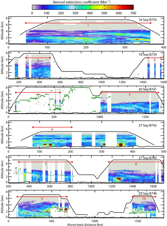
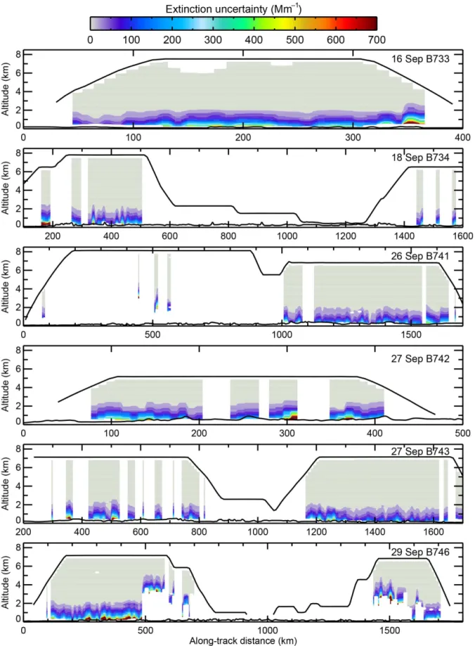
Figures 5 and 6 display the cross-sections of aerosol extinc-tion coefficient and of its estimated uncertainty, as a func-tion of along-track distance and height. Generally, all six flights show a similar structure, with a moderate magnitude of aerosol extinction, of the order of 150–200 Mm−1,
0 200 400 600 0
2 4 6 8
Altitude (km)
14:12 16 Sep B733 922’S 6609’W
0 200 400 600
0 2 4 6
8 12:44 18 Sep B734
1119’S 6329’W
0 200 400 600
0 2 4 6
8 14:50 26 Sep B741
959’S 5432’W
0 200 400 600
Aerosol extinction (Mm-1)
0 2 4 6 8
Altitude (km)
13:12 27 Sep B742 1111’S 4711’W
0 200 400 600
Aerosol extinction (Mm-1)
0 2 4 6
8 20:34 27 Sep B743
940’S 5933’W
0 200 400 600
Aerosol extinction (Mm-1)
0 2 4 6
8 13:48 29 Sep B746
906’S 5957’W
Figure 4. A sample of the lidar vertical profiles of aerosol extinction coefficient, discussed in this paper. The green lines indicate the estimate of uncertainty. The red lines indicate the reference height interval used (different for each profile). The time, date, flight number and coordinates are indicated in the title to each plot. Each profile corresponds to an integration time of 1 min.
thousands of kilometres and persisted over the 2-week pe-riod studied here.
At smaller spatial scales, some noticeable features were observed, and are described as follows. Flight B742 shows four features where a large extinction coefficient (approach-ing 1000 Mm−1) is detected at an altitude of 1.25 km, at along-track distances of 115, 135, 310 and 360 km. These correspond to plumes from single fires that were seen from the cockpit. Since the aircraft was flying back and forth over the same area, these smoke plumes were all located within a maximum distance of ∼25 km from each other, and in fact the ones observed at 310 and 360 km along-track distance were at the same location.
Flight B743 also shows a plume from a single fire, cen-tred at an along-track distance of 1260 km; it extends from the surface to 2 km altitude and has a size of ∼50 km in
the along-track horizontal direction; in this plume a peak ex-tinction of 1270±40 Mm−1was encountered. Moreover, a
higher altitude feature is observed, well above the aerosol layer, and co-located with this intense plume but apparently disconnected from it: its altitude is 3.7–4 km, with a depth varying between 200 and 400 m (FWHM). Its horizontal ex-tent is of 270 km along-track, its aerosol optical depth (AOD) peaks 0.09, and its extinction coefficient peaks 300 Mm−1. The origin of this higher altitude feature is uncertain: it could have been released by the same fire at an earlier time, i.e. if the fire radiative power had been at anytime stronger; it may
also have originated from some other nearby fire; and finally it may have been transported over a longer distance.
Moreover, in flights B741 (first part) and B746 the pres-ence of clouds with tops at 2–4 km obscures the bottom part of the aerosol layer; above these clouds, large extinction coefficients are detected, peaking 1000–1500 Mm−1. These large values are likely to be either directly caused by nearby fires (hidden by the clouds themselves), or as a result of con-vective lifting and detraining of smoke into a layer around the cloud-top.
Figure 5.Cross-sections of the aerosol extinction coefficient determined from the lidar for the six research flights with a 1-min integration
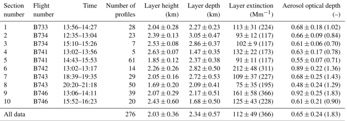
Table 2.Flight sections considered for the characterisation of the aerosol layer, displayed with red arrows in Fig. 5. For each section, the layer height, layer depth, layer extinction and aerosol optical depth are listed (see text). For each quantity, the average and standard deviation are shown; for the layer extinction and aerosol optical depth, maximum values are shown as well (in parentheses). The results for the whole data set are listed as well.
Section Flight Time Number of Layer height Layer depth Layer extinction Aerosol optical depth number number profiles (km) (km) (Mm−1) (–)
1 B733 13:56–14:27 28 2.04±0.28 2.27±0.23 113±31 (224) 0.68±0.18 (1.02)
2 B734 12:35–13:04 23 2.39±0.13 3.05±0.47 93±12 (117) 0.66±0.09 (0.84)
3 B734 15:10–15:26 7 2.53±0.08 2.86±0.37 102±9 (117) 0.61±0.06 (0.70)
4 B741 13:02–13:56 5 2.63±0.07 1.47±0.35 132±22 (173) 0.63±0.17 (0.78)
5 B741 14:43–15:53 61 1.85±0.12 2.37±0.38 91±11 (117) 0.55±0.07 (0.71)
6 B742 13:02–13:17 14 2.26±0.26 2.82±0.50 212±48 (311) 0.89±0.22 (1.36)
7 B743 18:39–19:35 29 2.05±0.16 2.72±0.53 109±37 (227) 0.68±0.25 (1.43)
8 B743 20:20–21:18 50 1.69±0.20 2.09±0.41 75±35 (195) 0.48±0.24 (1.29)
9 B746 13:06–14:11 39 2.07±0.29 2.17±0.51 161±58 (366) 0.92±0.25 (1.83)
10 B746 15:52–16:23 20 2.43±0.60 1.68±0.50 125±43 (228) 0.61±0.21 (0.90)
All data 276 2.03±0.36 2.34±0.57 112±49 (366) 0.65±0.24 (1.83)
to cloud) at a lower boundary which was 2.5 km or higher above mean sea level have not been included in the discus-sion of the derived quantities described above.
In order to characterise the aerosol layer in terms of repre-sentative properties, the data set has been divided in the sec-tions listed in Table 2, numbered 1–10, and also displayed with red arrows in Fig. 5. For each of the shorter flights, a single section has been considered, whereas when the dis-tance travelled exceeded 1000 km two flight sections have been considered. For flight B742, since the aircraft travelled back and forth over the same ground track several times, only the first part of the lidar cross-section has been considered. Due to the above quality criteria and to the fact that some flight portions have not been included (e.g. the second part of flight B742), the number of retained profiles is reduced from 334 to 276. Table 2 summarizes the flight sections averages and standard deviations for the considered quantities; note that in this context, standard deviation is a measure of vari-ability for each given quantity. The maximum of the layer ex-tinction and of the aerosol optical depth is also listed for each section; the maximum of the layer extinction is in general dif-ferent and lower than the maximum value of extinction that is encountered in each section (layer extinction being a ver-tically averaged quantity).
The geometrical properties of the aerosol vertical distri-bution, i.e. the layer height and layer depth, show a lim-ited variability within each section, with standard devia-tion around 10–15 % for layer height and 15–25 % for layer depth. Flight B746 represents an exception and shows larger variability in its second part (Sect. 10); however, for this flight a large proportion of profiles are truncated due to low cloud, and therefore the remaining data may possibly not provide a representative sample. Averaged over all six flights, the layer height is 2.0±0.4 km, and the layer depth is 2.3±0.6 (average and standard deviation). This indicates that
the vertical distribution of the aerosols does not vary much, despite the large distance travelled by the aircraft (more than 2200 km between the eastmost and westmost lidar profiles) and the relatively long time between the first and the last flight (14 days).
The quantitative properties, i.e. mean extinction and AOD, display a larger variability, as expected; however, this vari-ability is not huge. The per-section average of layer extinc-tion varies between 75 and 200 Mm−1 and the per-section
average of AOD is between 0.5 and 0.9, each of these quan-tities showing a standard deviation of 10–50 % in each flight section. When computed over all six flights, the average and standard deviation of these quantities is 112±49 Mm−1and
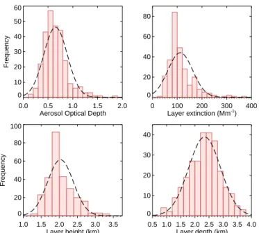
0.65±0.24, respectively, and the maximum values encoun-tered over the data set were about three times larger than the average. The distribution of the layer properties, derived by airborne lidar for the six flights considered in this paper, is shown in Fig. 7.
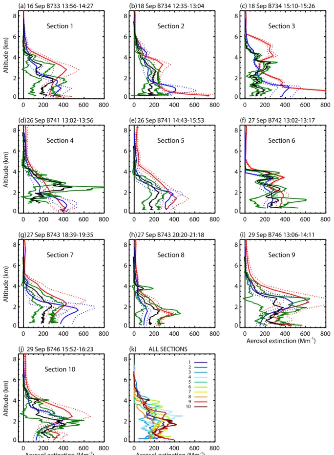
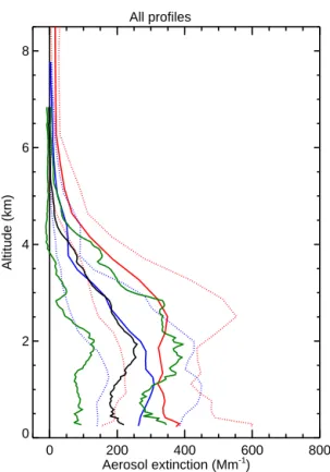
The mean vertical distributions of aerosol extinction for each of the ten sections are shown in Fig. 8. The average over the ten sections is displayed in Fig. 9, and shows a gen-eral structure that can be summarised as follows. Near the surface, and up to an altitude of∼1 km, a surface layer of
extinction coefficient∼200 Mm−1is observed. Above this
layer, an elevated layer is found which has a slightly larger extinction coefficient (peaking ∼250 Mm−1) and a
signif-icant depth, extending from∼1 to∼5 km altitude. When
0.0 0.5 1.0 1.5 2.0 Aerosol Optical Depth 0 10 20 30 40 50 60 Frequency
0 100 200 300 400
Layer extinction (Mm-1)
0 20 40 60 80
1.0 1.5 2.0 2.5 3.0 3.5
Layer height (km) 0 20 40 60 80 100 Frequency
0.5 1.0 1.5 2.0 2.5 3.0 3.5 4.0 Layer depth (km) 0
10 20 30 40
Figure 7.Distributions of aircraft lidar observations of AOD, layer
extinction, layer height and layer depth, for the whole data set con-sidered in this paper (276 vertical profiles). A Gaussian curve with the mean and standard deviation of the data set is superimposed (dashed line).
multi-layer atmosphere in the other sections. The signature of the individual fire plumes described above can be found in these average profiles; see e.g. the maximum at an altitude of ∼1.25 km in Sect. 6, and at an altitude of ∼1.6 km in Sect. 8. These layers also show a larger standard deviation, reflecting the variability between in-plume and out-of-plume conditions. Note also that Sects. 4, 9 and 10 are affected by low clouds with large smoke concentrations above; this is re-flected in the large values of the mean+1 standard deviation
(up to 600–800 Mm−1).
5 Model simulations
The lidar data have been used to evaluate aerosol simula-tions from two prediction models: (i) a limited area model (LAM) configuration of the Met Office Unified Model (Me-tUM), and (ii) aerosol forecasts issued by the European Cen-tre for Medium-range Weather Forecasts (ECMWF-MACC). The MetUM limited area model was set up for the SAMBBA campaign over the Amazonia domain (latitude 25◦S–18◦N, longitude 85–32◦W), and has a resolution of 12 km, with 70 levels in the vertical (Kolusu et al., 2015). Lateral bound-ary conditions for the meteorological fields were driven pro-vided by the operational global configuration of the MetUM (Global Atmosphere 3.1, Walters et al., 2011). The ECMWF-MACC simulations were global, although analysed here over the Amazonian region only. Both models were initialised us-ing near-real time emissions from the Global Fire Assimila-tion System (GFAS) emission data set (Kaiser et al., 2012),
valid for the forecast base time. The GFAS data are a daily product based on all the Moderate-Resolution Imaging Spec-troradiometer (MODIS) overpasses, over the course of any given day. Assimilation using this inventory is known to lead to an underestimation of AOD, due to the lack of detec-tion of small smouldering fires, and fires below canopies and clouds. Studies show that for a better agreement it is there-fore necessary to scale up the emissions (Kaiser et al., 2012). Whilst the ECMWF-MACC model used a scale factor of 3.4 (Kaiser et al., 2012), this was reduced to a factor of 1.7 for the MetUM based on an initial assessment of AODs with AERONET and MODIS data earlier in the season.
In the MetUM simulations, biomass burning aerosol was simulated on-line using the CLASSIC aerosol scheme (Bel-louin et al., 2011), while all other aerosol species were rep-resented by climatological averages. Direct aerosol effects were included in the simulations, but indirect effects were not. There are a number of uncertainties on some of the as-sumptions used in the simulations; in particular associated with the potential transport of aerosols from outside the do-main boundaries, the rainout of biomass burning aerosols and their ageing, and the source emissions. Aerosol injection was prescribed between 0.1 and 3 km in height; this is likely to affect the representation of the vertical extent of the aerosol plumes, in particular from larger fires. Moreover, emissions were not updated during the model simulation, and therefore an assumption is made on persistence of the emission field. The CLASSIC aerosol scheme uses a prescribed aerosol size distribution and refractive index, based on Haywood et al. (2003). A climatological hygroscopic growth curve based on Magi and Hobbs (2003) is included in the model, and this information enables the calculation of aerosol optical prop-erties, including extinction coefficient.
16 Sep B733 13:56-14:27
0 200 400 600 800
0 2 4 6 8
Altitude (km)
Section 1
(a) 18 Sep B734 12:35-13:04
0 200 400 600 800
0 2 4 6 8
Section 2
(b) 18 Sep B734 15:10-15:26
0 200 400 600 800
0 2 4 6 8
Section 3 (c)
26 Sep B741 13:02-13:56
0 200 400 600 800
0 2 4 6 8
Altitude (km)
Section 4
(d) 26 Sep B741 14:43-15:53
0 200 400 600 800
0 2 4 6 8
Section 5
(e) 27 Sep B742 13:02-13:17
0 200 400 600 800
0 2 4 6 8
Section 6 (f)
27 Sep B743 18:39-19:35
0 200 400 600 800
0 2 4 6 8
Altitude (km)
Section 7
(g) 27 Sep B743 20:20-21:18
0 200 400 600 800
0 2 4 6 8
Section 8
(h) 29 Sep B746 13:06-14:11
0 200 400 600 800
Aerosol extinction (Mm-1)
0 2 4 6 8
Section 9 (i)
29 Sep B746 15:52-16:23
0 200 400 600 800
Aerosol extinction (Mm-1)
0 2 4 6 8
Altitude (km)
Section 10
(j) ALL SECTIONS
0 200 400 600 800
Aerosol extinction (Mm-1)
0 2 4 6
8 1
2 3 4 5 6 7 8 9 10
(k)
Figure 8.Panels(a–j): summary vertical profiles for each of the 10 flight sections listed in Table 2. Each plot displays the mean vertical
profile (black) and the±1 standard deviation curves (green) for the lidar data. The MetUM (blue) and ECMWF-MACC (red) mean vertical
profiles and their standard deviation, for each of the sections, are also displayed. Panel(k): the 10 mean lidar vertical profiles shown in
All profiles
0 200 400 600 800
Aerosol extinction (Mm-1) 0
2 4 6 8
Altitude (km)
Figure 9. Lidar summary vertical profile resulting from all the
276 lidar profiles (black), together with the curves representing
±1 standard deviation (green). The MetUM (blue) and
ECMWF-MACC (red) mean vertical profiles and their standard deviation are also shown for the same collection of flight sections.
MODIS observations of Fire Radiative Power (FRP) and at-mospheric profiles from ECMWF; these are then gridded and assimilated in GFAS, and provided on a daily basis, together with emissions. Moreover, MODIS AOD data are routinely assimilated into the model, in a 4D-Var framework. All data are available online at http://www.copernicus-atmosphere. eu/. The resolution of the ECMWF model is∼80 km (T255),
coarser than that of the MetUM limited area model, and there are 60 model levels.
Figures 10 and 11 show the modelled aerosol extinction coefficient along the tracks of the six flights. Model clouds are also shown for the MetUM (green dashed contours); they are defined as the gridboxes where the cloud fraction is larger than 0.1 or the relative humidity is larger than 90 %.
The MetUM represents many realistic features of the aerosol layers, although plumes from individual fires are in some cases not captured. The ECMWF-MACC aerosol field is also realistic, but more smoothed out, as is expected due to its lower resolution.
The comparison between the airborne measurements and the MetUM is quite good for flight B733, where the model predicts elevated aerosol plumes, in good agreement with the observations. Differences appear, for instance, where the model predicts a slightly deeper aerosol layer and at
the same time it underestimates the extinction coefficient for the elevated layers. Similar intensities are found at 1.5– 2 km, although the features are not in exactly the same posi-tion as observed. The ECMWF-MACC model simulates the aerosols as being mainly concentrated in an elevated layer at
∼2.5 km, and as having a marked gradient, increasing with along-track distance (eastward). Overall, ECMWF-MACC overestimates the aerosol extinction in this case.
For the first part of flight B734 the lidar observes a rel-atively homogeneous layer from the surface up to 3–4 km, but with variations in its top altitude and some elevated thin plumes above. A similar distribution is highlighted in the MetUM and ECMWF-MACC models, although once again the exact position of the features is different. In the second part of this flight, however, the lidar highlights a deep el-evated plume at 2.5–4.5 km, with an extinction coefficient of the order of 200–250 Mm−1. As a comparison, we notice that the MetUM predicts some aerosol in the same place, al-though optically and geometrically thinner and with an irreg-ular structure within a cloudy field. The ECMWF-MACC, on the other hand, predicts a plume with a similar extinction but a higher altitude (4–6 km).
For flight B741, the difference between the models and the observations is remarkably more pronounced. In fact, for this case both models overestimate aerosols near the surface, and show a rapidly decreasing concentration above 3–4 km with a highly variable top of the aerosol layer reaching in some places up to∼7 km. In the first part of this flight very
little observational data were available, due to the presence of deep clouds; a few lidar profiles are however available, and they indicate an intense aerosol layer (400–700 Mm−1) at 2– 4 km, hence with much larger altitude than the main layer in both model outputs. In the second part of this flight, the top of the aerosol layer at 3–4 km is much sharper than in the model predictions, with most of the aerosols being found between
∼1 and∼3 km.
For flight B742, the MetUM shows a slightly smaller aerosol extinction coefficient than the lidar observations, and a slightly shallower aerosol layer, but overall the vertical dis-tribution is well represented, with the exception of the indi-vidual fire plumes, that appear much fainter. For the same flight ECMWF-MACC shows larger extinction values.
Figure 10.Cross-sections of the aerosol extinction coefficient estimated from the Met Office Unified Model (MetUM) along the tracks of
Figure 11.Cross-sections of the aerosol extinction coefficient estimated from the ECMWF-MACC model, along the tracks of the six research
not surprising, as the fire was not captured in the GFAS in-ventory.
Finally, for B746 the overall structure and magnitude of the smoke layer observed by the lidar is surprisingly well rep-resented in both models, with the exception of the very large values of extinction found just above the low-level clouds.
Some of the largest discrepancies between the models and the observations occur in regions affected by clouds; for in-stance during B741 (first part, Sect. 4) and B746 (large ex-tinction values above and near the clouds). This may be due to differences in location between modelled and observed convection (and associated transport and/or wet deposition of aerosol), or to errors in the water uptake of aerosols near to, or within clouds. This should not be considered surpris-ing, as these processes are difficult to model accurately, and still not well understood.
The blue and red lines in Figs. 8 and 9 show the MetUM and ECMWF-MACC mean and standard deviation, for each flight section and for the campaign average profile. These vertical profiles confirm the above conclusions; it is interest-ing, in any case, to observe the similarity of the campaign av-erage profile derived with the lidar and the MetUM (Fig. 9). Although the MetUM average does not seem to capture the transition between the first shallow layer (up to∼1 km) and
the elevated layer between∼1 and∼5 km, such an elevated
layer is shown clearly in most of the profiles in Fig. 8 (flight sections 1, 3, 5, and 7–10), but by averaging over multi-ple profiles with opposite structures (e.g. section 4) this is not apparent. Note also the structure of the campaign mean ECMWF-MACC profile, with a nearly constant extinction coefficient from the surface to 3 km, followed by a decrease until the top of the layer at∼6 km. Again, this results from averaging profiles with opposite structures, i.e. sections 2, 3 and 4, showing very large concentrations near the surface, and sections 1, and 5–10 that show larger extinction in the elevated layer. It is also clear from the averaged profiles that the ECMWF-MACC model shows larger aerosol extinction than the lidar and the MetUM, and that the simulated layers extend slightly further in the vertical.
Finally, Fig. 12 shows the hotspots reported in GFAS dur-ing the campaign, coloured accorddur-ing to the injection height computed in the PRM. We can see that several fires with in-jection height between 3 and 5 km are observed, particularly in the eastern (upwind) part of the basin, and this is where the smoke can have been generated. Moreover, sporadic fires with very large injection heights (5–7 km) are observed be-tween 50 and 65◦W. The smoke layer depths observed by li-dar and predicted by the models are therefore generally com-patible with the PRM injection heights.
6 Summary and conclusions
Research flights in Brazil, during SAMBBA (dry season of 2012), offered an opportunity to map the vertical structure
-20 -15 -10 -5 0
Latitude
16-22 Sep
0 1 2 3 4 5 6 Injection
height (km)
-75 -70 -65 -60 -55 -50 -45
Longitude -20
-15 -10 -5 0
Latitude
23-29 Sep
Figure 12. Hotspots during 16–22 September (top) and 23–
29 September (bottom), as reported in the GFAS inventory. Each hotspot is coloured according to the corresponding injection height computed by the plume rise model embedded in GFAS.
of the Amazonian haze using airborne lidar. The sampling region extended ∼2200 km along an east–west direction,
centred around a mean latitude of 10◦S, and the sampling period was 14-days long. Lidar profiles underwent cloud screening and a series of quality tests, including a man-ual profile-by-profile review of the reference height inter-val and cloud screening. High loadings of biomass burning aerosol were present, with an average AOD of 0.65±0.24 and a layer extinction (vertically averaged aerosol extinction) of 112±49 Mm−1. Within the main aerosol layers, the ex-tinction was often much larger than this, and ranged 100– 400 Mm−1 typically, and reaching values as high as 1000– 1500 Mm−1locally.
multiple layers were observed. On average, across the data set considered here the layer height was 2.0±0.4 km and the layer depth was 2.3±0.6 km (mean and standard devi-ation). This general structure is likely to be a consequence of dynamical processes, such as initial plume-rise, vertical transport by dry and moist convection, and large-scale mo-tion. Lifting of the aerosols from the surface can be explained with fire radiative power; see e.g. the plumes in B743, at an along-track distance of 1260 km, where lifting up to 2–3 km is evident, with an additional plume at ∼4 km. In this
re-spect, the injection heights computed in the PRM (Fig. 12), display a general consistency with the plume depths reported in the present study. Considering the large number of con-vective clouds encountered during SAMBBA (mainly in the western half of the area sampled), updrafts in cumulus and cumulonimbus can also be ascribed as a mechanism for lift-ing smoke above the boundary layer.
The mean vertical distribution of the aerosols that we ob-served is not too dissimilar to the results of other studies, such as Baars et al. (2012, Figs. 5 and 14), Huang et al. (2015, Fig. 6a and b), and Bourgeois et al. (2015, Fig. 6e); note, however, than in the latter paper the aerosols were found to be mainly in the boundary layer, below 2–2.5 km. The gen-eral vertical structure that we have found was fairly consis-tent across the region sampled (which extended∼2200 km
in an East-West direction) and across the time period con-sidered (14 days). As an exception to this, very large aerosol loads were found (extinction 1000–1500 Mm−1and AOD 1– 1.8) in two circumstances: (i) in individual fire plumes, and (ii) in the vicinity of clouds. The latter circumstance suggests either the uptake of water by aerosol close to clouds (Koren et al., 2007), or that smoke has been transported vertically within convective clouds and detrained to form elevated lay-ers with locally high aerosol extinction coefficient.
An evaluation of the biomass burning lidar ratio has also been completed, using the lidar profiles themselves. Consis-tency of the observed profiles with Rayleigh scattering above the aerosol layers permitted the lidar ratio to be estimated as 73±6 sr. This estimate has been compared with Mie
scatter-ing calculations usscatter-ing the campaign mean size-distribution obtained from wing-mounted optical particle counters. It has been found that the computed lidar ratio is very dependent upon the refractive index, and indeed the observed value is compatible with values of the real and imaginary parts pub-lished in the literature.
The present research effort has been a good opportunity for a general test of the Marenco (2013) inversion method, and it represents its first application to a large number of lidar profiles. This method is a variant of the traditional Fernald-Klett approach, where a far-range reference is taken within an aerosol layer instead of in a Rayleigh scattering portion of the atmosphere (the latter being only available at near-range, leading to retrieval instabilities). The method is suit-able for the observation of deep and optically thick layers, when observed in a nadir-viewing geometry. A
profile-by-profile evaluation of the uncertainties introduced by the in-version assumptions has been included. These uncertainties are shown in Fig. 6 and can approach values as large as 50– 100 % near the surface, but they are much reduced at altitudes larger than 1–2 km.
The observed structure of the aerosol layer has been com-pared to predictions with a limited-area configuration of the MetUM and with the ECMWF-MACC global model. In most cases, the models represented the general vertical structure of the aerosol layers and showed realistic features, such as layer depth and magnitude of the extinction coefficient. For instance, in many cases the models showed a similar aerosol layer depth, and a similar magnitude of the extinction coef-ficient, although some differences exist, and the exact posi-tion of features was not always exactly reproduced. Certain features, such as individual fire plumes and high extinction values in the vicinity of clouds, were however not well cap-tured.
We believe that it is important to highlight the strengths and weaknesses of the models in predicting the vertical struc-ture, because the latter is usually considered a weak point. It is to be noted that the MetUM SAMBBA LAM was set up specifically to support the field campaign, and its primary purpose was to facilitate flight planning, whereas the pur-pose of the ECMWF-MACC simulations is somewhat differ-ent. The latter is an operational global composition model, with forecast charts made available publicly on the web on a daily basis, and for which specially zoomed charts can be re-quested for campaign support. In both cases, the simulations are judged to be useful if they provide some skill in predict-ing the typical vertical distribution of the aerosol, the regional distribution, and the day-to-day variability of aerosol load-ings. Our results show some skill in simulating these aspects, even if the fine detail is not always captured, and we conclude that the simulations have served their purpose well.
indication that the emission scaling factors used (1.7 for the MetUM and 3.4 for ECMWF-MACC) is reasonable.
Kolusu et al. (2015) have also investigated the impact of the prognostic biomass burning aerosols on the meteorol-ogy simulated with the MetUM. They have found an impact on the radiation balance, improvements in forecasts of tem-perature and humidity, and they have highlighted important changes in the representation of the regional hydrological cy-cle. In this respect, we believe that the vertical profile of the aerosols is a key variable to take into account, and that our data set can prove precious for such studies.
In the ECMWF-MACC model, injection heights are sulated interactively from the PRM, and this led to some im-provements in the vertical profile of aerosol for flights B741, B742 and B746. A separate paper on this topic is in prepa-ration (Rémy et al., 2015), and therein it will be shown that, e.g., for flight B742 the simulation using the PRM is able to predict the two distinct smoke layers that were observed, whereas only one broader layer is predicted if the PRM is not used.
In conclusion, the airborne lidar has once again proven to be a powerful tool for mapping aerosols along the verti-cal and horizontal axes. The ability to vertiverti-cally profile the atmosphere yields an advantage over passive remote sens-ing, in that the atmospheric structure can be resolved, and moreover the observed signal is not sensitive to parameters such as layer temperature and ground reflection or emission. Lidar permits sampling of the whole atmospheric column, and thus to retrieve a complete picture of the atmospheric structure, and is thus complementary to in situ techniques that can yield more detailed microphysical information but on a smaller spatial scale. We believe that our study also il-lustrates well the application of lidar observations to model verification and assessment, and it opens the door to a series of further studies: besides the above-mentioned evaluation of the GFAS inventory (Rémy et al., 2015), we are also working on an evaluation of the UKCA-MODE aerosol scheme in the Met Office climate model (Johnson et al., 2016).
Acknowledgements. Airborne data were obtained using the BAe-146-301 Atmospheric Research Aircraft (ARA) flown by Directflight Ltd and managed by the Facility for Airborne Atmospheric Measurements (FAAM), which is a joint entity of the Natural Environment Research Council (NERC) and the Met Office. SAMBBA was funded by the Met Office and NERC (grant NE/J009822/1). Patrick Chazette and the Commissariat à l’Energie Atomique et aux Energies Alternatives (CEA) are kindly thanked for help fixing our lidar prior to SAMBBA.
Edited by: S. Martin
References
Abel, S. J., Haywood, J. M., Highwood, E. J., Li, J., and Buseck, P. R.: Evolution of biomass burning aerosol properties from an agricultural fire in southern Africa, Geophys. Res. Lett., 30, 1783, doi:10.1029/2003GL017342, 2003.
Allen, G., Illingworth, S. M., O’Shea, S. J., Newman, S., Vance, A., Bauguitte, S. J.-B., Marenco, F., Kent, J., Bower, K., Gal-lagher, M. W., Muller, J., Percival, C. J., Harlow, C., Lee, J., and Taylor, J. P.: Atmospheric composition and thermodynamic re-trievals from the ARIES airborne TIR-FTS system – Part 2: Val-idation and results from aircraft campaigns, Atmos. Meas. Tech., 7, 4401–4416, doi:10.5194/amt-7-4401-2014, 2014.
Andreae, M. O., Rosenfeld, D., Artaxo, P., Costa, A. A., Frank, G. P., Longo, K. M., and Silva-Dias, M. A. F.: Smoking Rain Clouds over the Amazon, Science, 303, 1337–1342, 2004. Angelo, C.: Amazon fire analysis hits new heights, Nature News,
doi:10.1038/nature.2012.11467, 2012.
Baars, H., Ansmann, A., Althausen, D., Engelmann, R., Heese, B., Müller, D., Artaxo, P., Paixao, M., Pauliquevis, T., and Souza, R.: Aerosol profiling with lidar in the Amazon Basin during the wet and dry season, J. Geophys. Res., 117, D21201, doi:10.1029/2012JD018338, 2012.
Bellouin, N., Rae, J., Jones, A., Johnson, C., Haywood, J., and Boucher, O.: Aerosol forcing in the Climate Model Intercom-parison Project (CMIP5) simulations by HadGEM2-ES and the role of ammonium nitrate, J. Geophys. Res., 116, D20206, doi:10.1029/2011JD016074, 2011.
Benedetti, A., Morcrette, J.-J., Boucher, O., Dethof, A., Engelen, R. J., Fisher, M., Flentje, H., Huneeus, N., Jones, L., Kaiser, J. W., Kinne, S., Mangold, A., Razinger, M., Simmons, A. J., and Suttie, M.: , Aerosol analysis and forecast in the European Centre for Medium-Range Weather Forecasts Integrated Forecast System: 2. Data assimilation, J. Geophys. Res., 114, D13205, doi:10.1029/2008JD011115, 2009.
Boucher, O., Pham, M., and Venkataraman, C.: Simulation of the atmospheric sulfur cycle in the Laboratoire de Meteorologie Dy-namique general circulation model: Model description, model evaluation, and global and European budgets, Institut Pierre Si-mon Laplace (Note Sci. IPSL 23), Paris, France, 2002.
Bourgeois, Q., Ekman, A. M. L., and Krejci, R.: Aerosol transport over the Andes from the Amazon Basin to the remote Pacific Ocean: A multiyear CALIOP assessment, J. Geophys. Res., 120, 8411–8425, 2015.
Brito, J., Rizzo, L. V., Morgan, W. T., Coe, H., Johnson, B., Hay-wood, J., Longo, K., Freitas, S., Andreae, M. O., and Artaxo, P.: Ground-based aerosol characterization during the South Amer-ican Biomass Burning Analysis (SAMBBA) field experiment, Atmos. Chem. Phys., 14, 12069–12083, doi:10.5194/acp-14-12069-2014, 2014.
Chand, D., Anderson, T. L., Wood, R., Charlson, R. J., Hu, Y., Liu, Z., and Vaughan, M.: Quantifying above-cloud aerosol us-ing spaceborne lidar for improved understandus-ing of cloudy-sky direct climate forcing, J. Geophys. Res., 113, D13206, doi:10.1029/2007JD009433, 2008.
Dubovik, O., Holben, B., Eck, T. F., Smirnov, A., Kaufman, Y. J., King, M. D., Tanré, D., and Slutsker, I.: Variability of absorption and optical properties of key aerosol types observed in world-wide locations, J. Atmos. Sci., 59, 590–608, 2002.
Fernald, F. G.: Analysis of atmospheric lidar observations: some comments, Appl. Opt., 23, 652–653, 1984.
Fiebig, M., Stohl, A., Wendisch, M., Eckhardt, S., and Petzold, A.: Dependence of solar radiative forcing of forest fire aerosol on ageing and state of mixture, Atmos. Chem. Phys., 3, 881–891, doi:10.5194/acp-3-881-2003, 2003.
Freitas, S. R., Longo, K. M., Chatfield, R., Latham, D., Silva Dias, M. A. F., Andreae, M. O., Prins, E., Santos, J. C., Gielow, R., and Carvalho Jr., J. A.: Including the sub-grid scale plume rise of veg-etation fires in low resolution atmospheric transport models, At-mos. Chem. Phys., 7, 3385–3398, doi:10.5194/acp-7-3385-2007, 2007.
Gerbig, C., Kley, D., Volz-Thomas, A., Kent, J., Dewey, K., and McKenna, D. S.: Fast response resonance fluorescence CO mea-surements aboard the C-130: Instrument characterization and measurements made during North Atlantic Regional Experiment 1993, J. Geophys. Res., 101, 29229–29238, 1996.
Gerbig, C., Schmitgen, S., Kley, D., Volz-Thomas, A., Dewey, K., and Haaks, D.: An improved fast-response vacuum-UV reso-nance fluorescence CO instrument, J. Geophys. Res., 104, 1699– 1704, 1999.
Gonçalves, W. A., Machado, L. A. T., and Kirstetter, P.-E.: Influence of biomass aerosol on precipitation over the Central Amazon: an observational study, Atmos. Chem. Phys., 15, 6789–6800, doi:10.5194/acp-15-6789-2015, 2015.
Groß, S., Freudenthaler, V., Wiegner, M., Gasteiger, J., Geiß, A., and Schnell, F.: Dual-wavelength linear depolarization ratio of volcanic aerosols: Lidar measurements of the Eyjafjallajökull plume over Maisach, Germany, Atmos. Environ., 48, 85–96, 2012.
Guyon, P., Graham, B., Beck, J., Boucher, O., Gerasopoulos, E., Mayol-Bracero, O. L., Roberts, G. C., Artaxo, P., and Andreae, M. O.: Physical properties and concentration of aerosol parti-cles over the Amazon tropical forest during background and biomass burning conditions, Atmos. Chem. Phys., 3, 951–967, doi:10.5194/acp-3-951-2003, 2003.
Haywood, J. M., Osborne, S. R., Francis, P. N., Keil, A., Formenti, P., Andreae, M. O., and Kaye, P. H.: The mean physical and op-tical properties of regional haze dominated by biomass burning aerosol measured from the C-130 aircraft during SAFARI 2000, J. Geophys. Res., 108, 8473, doi:10.1029/2002JD002226, 2003. Hobbs, P. V., Reid, J. S., Kotchenruther, R. A., Ferek, R. J., and Weiss, R.: Direct radiative forcing by smoke from biomass burn-ing, Science, 275, 1777–1778, 1997.
Huang, J., Guo, J., Wang, F., Liu, Z., Jeong, M.-J., Yu, H., and Zhang, Z.: CALIPSO inferred most probable heights of global dust and smoke layers, J. Geophys. Res., 120, 5085–5100, 2015. Johnson, B., Haywood, J., Langridge, J., Darbyshire, E., Morgan, W., Szpeck, K., Brooke, J., Marenco, F., Coe, H., Artaxo, P., Longo, K., Mulcahy, J., Mann, G., Dalvi, M., and Bellouin, N.: Evaluation of biomass burning aerosols in the HadGEM3 climate model with observations from SAMBBA, Atmos. Chem. Phys. Discuss., in preparation, 2016.
Kaiser, J. W., Heil, A., Andreae, M. O., Benedetti, A., Chubarova, N., Jones, L., Morcrette, J.-J., Razinger, M., Schultz, M. G., Suttie, M., and van der Werf, G. R.: Biomass burning emis-sions estimated with a global fire assimilation system based on observed fire radiative power, Biogeosciences, 9, 527–554, doi:10.5194/bg-9-527-2012, 2012.
Kaufman, Y. J., Hobbs, P. V., Kirchhoff, V. W. J. H., Artaxo, P., Remer, L. A., Holben, B. N., King, M. D., Ward, D. E., Prins, E. M., Longo, K. M., Mattos, L. F., Nobre, C. A., Spinhirne, J. D., Ji, Q., Thompson, A. M., Gleason, J. F., Christopher, S. A., and Tsay, S.-C.: Smoke, Clouds, and Radiation-Brazil (SCAR-B) experiment, J. Geophys. Res., 103, 31783–31808, 1998. Klett, J. D.: Lidar inversion with variable backscatter/extinction
ra-tios, Appl. Opt., 24, 1638–1643, 1985.
Kolusu, S. R., Marsham, J. H., Mulcahy, J., Johnson, B., Dun-ning, C., Bush, M., and Spracklen, D. V.: Impacts of Ama-zonia biomass burning aerosols assessed from short-range weather forecasts, Atmos. Chem. Phys., 15, 12251–12266, doi:10.5194/acp-15-12251-2015, 2015.
Koppmann, R., von Czapiewski, K., and Reid, J. S.: A review of biomass burning emissions, part I: gaseous emissions of carbon monoxide, methane, volatile organic compounds, and nitrogen containing compounds, Atmos. Chem. Phys. Discuss., 5, 10455– 10516, doi:10.5194/acpd-5-10455-2005, 2005.
Koren, I., Remer, L. A., Kaufman, Y. J., Rudich, Y., and Martins, J. V.: On the twilight zone between clouds and aerosols, Geo-phys. Res. Lett., 34, L08805, doi:10.1029/2007GL029253, 2007. Koren, I., Martins, J. V., Remer, L. A., and Afargan, H.: Smoke Invigoration Versus Inhibition of Clouds over the Amazon, Sci-ence, 321, 946–949, 2008.
Labonne, M., Breon, F.-M., and Chevallier, F.: Injection height of biomass burning aerosols as seen from a spaceborne lidar, Geo-phys. Res. Lett., 34, L11806, doi:10.1029/2007GL029311, 2007. Lance, S., Brock, C. A., Rogers, D., and Gordon, J. A.: Water droplet calibration of the Cloud Droplet Probe (CDP) and in-flight performance in liquid, ice and mixed-phase clouds during ARCPAC, Atmos. Meas. Tech., 3, 1683–1706, doi:10.5194/amt-3-1683-2010, 2010.
Liu, P. S. K., Leaitch, W. R., Strapp, J. W., and Wasey, M. A.: Response of particle measuring systems airborne ASASP and PCASP to NaCl and latex particles, Aerosol Sci. Tech., 16, 83– 95, 1992.
Lolli, S., Sauvage, L., Loaec, S., and Lardier, M.: EZ Lidar(TM): A new compact autonomous eye-safe scanning aerosol lidar for extinction measurements and PBL height detection. Validation of the performances against other instruments and intercomparison campaigns, Óptica Pura y Aplicada, 44, 33–41, 2011.
Lopes, F. J. S., Landulfo, E., and Vaughan, M. A.: Evaluat-ing CALIPSO’s 532 nm lidar ratio selection algorithm usEvaluat-ing AERONET sun photometers in Brazil, Atmos. Meas. Tech., 6, 3281–3299, doi:10.5194/amt-6-3281-2013, 2013.
Magi, B. and Hobbs, P. V.: Effects of humidity on aerosols and southern Africa during the biomass burning season, J. Geophys. Res., 108, 8495, doi:10.1029/2002JD002144, 2003.
Marenco, F., Johnson, B., Turnbull, K., Newman, S., Haywood, J., Webster, H., and Ricketts, H.: Airborne Lidar Observations of the 2010 Eyjafjallajökull Volcanic Ash Plume, J. Geophys. Res., 116, D00U05, doi:10.1029/2011JD016396, 2011.
Marenco, F., Amiridis, V., Marinou, E., Tsekeri, A., and Pelon, J.: Airborne verification of CALIPSO products over the Amazon: a case study of daytime observations in a complex atmospheric scene, Atmos. Chem. Phys., 14, 11871–11881, doi:10.5194/acp-14-11871-2014, 2014.
Mattis, I., Ansmann, A., Wandinger, U., and Müller, D.: Unex-pectedly high aerosol load in the free troposphere over central Europe in spring/summer 2003, Geophys. Res. Lett., 30, 2178, doi:10.1029/2003GL018442, 2003.
Mercado, L. M., Bellouin, N., Sitch, S., Boucher, O., Huntingford, C., Wild, M., and Cox, P. M.: Impact of changes in diffuse ra-diation on the global land carbon sink, Nature, 458, 1014–1017, 2009.
Morcrette, J.-J., Boucher, O., Jones, L., Salmond, D., Bechtold, P., Beljaars, A., Benedetti, A., Bonet, A., Kaiser, J. W., Razinger, M., Schulz, M., Serrar, S., Simmons, A. J., Sofiev, M., Suttie, M., Tompkins, A. M., and Untch, A.: Aerosol analysis and forecast in the European Centre for Medium-Range Weather Forecasts In-tegrated Forecast System: Forward modeling, J. Geophys. Res., 114, D06206, doi:10.1029/2008JD011235, 2009.
Müller, D., Mattis, I., Wandinger, U., Ansmann, A., Althausen, D., and Stohl, A.: Raman lidar observations of aged Siberian and Canadian forest fire smoke in the free troposphere over Ger-many in 2003: Microphysical particle characterization, J. Geo-phys. Res., 110, D17201, doi:10.1029/2004JD005756, 2005. Omar, A. H., Winker, D. M., Kittaka, C., Vaughan, M. A., Liu, Z.,
Hu, Y., Trepte, C. R., Rogers, R. R., Ferrare, R. A., Lee, K.-P., Kuehn, R. E., and Hostetler, C. A.: The CALIPSO Automated Aerosol Classification and Lidar Ratio Selection Algorithm, J. Atmos. Ocean. Tech., 26, 1994–2014, 2009.
Palmer, P. I., Parrington, M., Lee, J. D., Lewis, A. C., Rickard, A. R., Bernath, P. F., Duck, T. J., Waugh, D. L., Tarasick, D. W., Andrews, S., Aruffo, E., Bailey, L. J., Barrett, E., Bauguitte, S. J.-B., Curry, K. R., Di Carlo, P., Chisholm, L., Dan, L., Forster, G., Franklin, J. E., Gibson, M. D., Griffin, D., Helmig, D., Hop-kins, J. R., Hopper, J. T., Jenkin, M. E., Kindred, D., Kliever, J., Le Breton, M., Matthiesen, S., Maurice, M., Moller, S., Moore, D. P., Oram, D. E., O’Shea, S. J., Owen, R. C., Pagniello, C. M. L. S., Pawson, S., Percival, C. J., Pierce, J. R., Punjabi, S., Purvis, R. M., Remedios, J. J., Rotermund, K. M., Sakamoto, K. M., da Silva, A. M., Strawbridge, K. B., Strong, K., Taylor, J., Trigwell, R., Tereszchuk, K. A., Walker, K. A., Weaver, D., Whaley, C., and Young, J. C.: Quantifying the impact of BO-Real forest fires on Tropospheric oxidants over the Atlantic us-ing Aircraft and Satellites (BORTAS) experiment: design, execu-tion and science overview, Atmos. Chem. Phys., 13, 6239–6261, doi:10.5194/acp-13-6239-2013, 2013.
Paugam, R., Wooster, M., Atherton, J., Freitas, S. R., Schultz, M. G., and Kaiser, J. W.: Development and optimization of a wildfire plume rise model based on remote sensing data in-puts – Part 2, Atmos. Chem. Phys. Discuss., 15, 9815–9895, doi:10.5194/acpd-15-9815-2015, 2015.
Reddy, M. S., Boucher, O., Bellouin, N., Schulz, M., Balkan-ski, Y., Dufresne, J.-L., and Pham, M.: Estimates of global multicomponent aerosol optical depth and direct radiative
perturbation in the Laboratoire de Meteorologie Dynamique general circulation model, J. Geophys. Res., 110, D10S16, doi:10.1029/2004JD004757, 2005.
Reid, J. S. and Hobbs, P. V.: Physical and optical properties of young smoke from individual biomass fires in Brazil, J. Geophys. Res., 103, 32013–32030, 1998.
Reid, J. S., Eck, T. F., Christopher, S. A., Koppmann, R., Dubovik, O., Eleuterio, D. P., Holben, B. N., Reid, E. A., and Zhang, J.: A review of biomass burning emissions part III: intensive optical properties of biomass burning particles, Atmos. Chem. Phys., 5, 827–849, doi:10.5194/acp-5-827-2005, 2005a.
Reid, J. S., Koppmann, R., Eck, T. F., and Eleuterio, D. P.: A review of biomass burning emissions part II: intensive physical proper-ties of biomass burning particles, Atmos. Chem. Phys., 5, 799– 825, doi:10.5194/acp-5-799-2005, 2005b.
Rémy, S., Veira, A., Paugam, R., Kaiser, J., Marenco, F., Burton, S., Benedetti, A., Engelen, R., Ferrare, R., and Hair, J.: Two global climatologies of daily fire emission injection heights since 2003, Atmos. Chem. Phys., submitted, 2015.
Rizzo, L. V., Artaxo, P., Müller, T., Wiedensohler, A., Paixão, M., Cirino, G. G., Arana, A., Swietlicki, E., Roldin, P., Fors, E. O., Wiedemann, K. T., Leal, L. S. M., and Kulmala, M.: Long term measurements of aerosol optical properties at a primary forest site in Amazonia, Atmos. Chem. Phys., 13, 2391–2413, doi:10.5194/acp-13-2391-2013, 2013.
Rosenberg, P. D., Dean, A. R., Williams, P. I., Dorsey, J. R., Minikin, A., Pickering, M. A., and Petzold, A.: Particle sizing calibration with refractive index correction for light scattering optical particle counters and impacts upon PCASP and CDP data collected during the Fennec campaign, Atmos. Meas. Tech., 5, 1147–1163, doi:10.5194/amt-5-1147-2012, 2012.
Ryder, C. L., Highwood, E. J., Rosenberg, P. D., Trembath, J., Brooke, J. K., Bart, M., Dean, A., Crosier, J., Dorsey, J., Brind-ley, H., Banks, J., Marsham, J. H., McQuaid, J. B., Sodemann, H., and Washington, R.: Optical properties of Saharan dust aerosol and contribution from the coarse mode as measured during the Fennec 2011 aircraft campaign, Atmos. Chem. Phys., 13, 303– 325, doi:10.5194/acp-13-303-2013, 2013.
Seifert, P., Kunz, C., Baars, H., Ansmann, A., Bühl, J., Senf, F., Engelmann, R., Althausen, D., and Artaxo, P.: Seasonal variabil-ity of heterogeneous ice formation in stratiform clouds over the Amazon Basin, Geophys. Res. Lett., 42, 5587–5593, 2015. Sena, E. T., Artaxo, P., and Correia, A. L.: Spatial variability of
the direct radiative forcing of biomass burning aerosols and the effects of land use change in Amazonia, Atmos. Chem. Phys., 13, 1261–1275, doi:10.5194/acp-13-1261-2013, 2013.
Sofiev, M., Ermakova, T., and Vankevich, R.: Evaluation of the smoke-injection height from wild-land fires using remote-sensing data, Atmos. Chem. Phys., 12, 1995–2006, doi:10.5194/acp-12-1995-2012, 2012.
Stocker, T. F., Qin, D., Plattner, G.-K., Tignor, M. M., Allen, S. K., Boschung, J., Nauels, A., Xia, Y., Bex, V., and Midgley, P. M.: Climate change 2013: The physical science basis, unedited on-line version, available at: www.ipcc.ch/report/ar5/wg1/ (last ac-cess: 19 February 2016), 2013.
Isaksen, I., Iversen, I., Kloster, S., Koch, D., Kirkevåg, A., Krist-jansson, J. E., Krol, M., Lauer, A., Lamarque, J. F., Liu, X., Mon-tanaro, V., Myhre, G., Penner, J., Pitari, G., Reddy, S., Seland, Ø., Stier, P., Takemura, T., and Tie, X.: Analysis and quantifica-tion of the diversities of aerosol life cycles within AeroCom, At-mos. Chem. Phys., 6, 1777–1813, doi:10.5194/acp-6-1777-2006, 2006.
Vakkari, V., Kerminen, V.-M., Beukes, J. P., Tiitta, P., van Zyl, P. G., Josipovic, M., Venter, A. D., Jaars, K., Worsnop, D. R., Kulmala, M., and Laakso, L.: Rapid changes in biomass burning aerosols by atmospheric oxidation, Geophys. Res. Lett., 41, 2644–2651, 2014.