Mixed Signal Learning by Spike Correlation
Propagation in Feedback Inhibitory Circuits
Naoki Hiratani1,2*, Tomoki Fukai2*
1Department of Complexity Science and Engineering, The University of Tokyo, Kashiwa, Chiba, Japan, 2Laboratory for Neural Circuit Theory, RIKEN Brain Science Institute, Wako, Saitama, Japan
*[email protected](NH); [email protected](TF)
Abstract
The brain can learn and detect mixed input signals masked by various types of noise, and spike-timing-dependent plasticity (STDP) is the candidate synaptic level mechanism. Be-cause sensory inputs typically have spike correlation, and local circuits have dense feed-back connections, input spikes cause the propagation of spike correlation in lateral circuits; however, it is largely unknown how this secondary correlation generated by lateral circuits influences learning processes through STDP, or whether it is beneficial to achieve efficient spike-based learning from uncertain stimuli. To explore the answers to these questions, we construct models of feedforward networks with lateral inhibitory circuits and study how propagated correlation influences STDP learning, and what kind of learning al-gorithm such circuits achieve. We derive analytical conditions at which neurons detect minor signals with STDP, and show that depending on the origin of the noise, different cor-relation timescales are useful for learning. In particular, we show that non-precise spike correlation is beneficial for learning in the presence of cross-talk noise. We also show that by considering excitatory and inhibitory STDP at lateral connections, the circuit can ac-quire a lateral structure optimal for signal detection. In addition, we demonstrate that the model performs blind source separation in a manner similar to the sequential sampling ap-proximation of the Bayesian independent component analysis algorithm. Our results pro-vide a basic understanding of STDP learning in feedback circuits by integrating analyses from both dynamical systems and information theory.
Author Summary
In natural environments, although sensory inputs are often highly mixed with one an-other and obscured by noise, animals can detect and learn discrete signals from this mix-ture. For example, humans easily detect the mention of their names from across a noisy room, a phenomenon known as the cocktail party effect. Spike-timing-dependent plas-ticity (STDP) is a learning mechanism ubiquitously observed in the brain across various species and is considered to be the neural basis of such learning; however, it is still un-clear how STDP enables efficient learning from uncertain stimuli and whether spike-based learning offers benefits beyond those provided by standard machine learning OPEN ACCESS
Citation:Hiratani N, Fukai T (2015) Mixed Signal Learning by Spike Correlation Propagation in Feedback Inhibitory Circuits. PLoS Comput Biol 11(4): e1004227. doi:10.1371/journal.pcbi.1004227
Editor:Abigail Morrison, Research Center Jülich, GERMANY
Received:December 2, 2014
Accepted:March 6, 2015
Published:April 24, 2015
Copyright:© 2015 Hiratani, Fukai. This is an open access article distributed under the terms of the Creative Commons Attribution License, which permits unrestricted use, distribution, and reproduction in any medium, provided the original author and source are credited.
Data Availability Statement:All relevant data are within the paper and its Supporting Information files.
Introduction
Neurons receive inputs from a large number of other neurons encoding a variety of informa-tion about various signals. Despite the diversity and variability of input spike trains, neurons can learn and represent specific information during developmental processes and according to specific task requirements. Spike-timing-dependent plasticity (STDP) [1,2] is a candidate mechanism of neural learning. Extensive studies have revealed the type of information that a single neuron can learn through STDP [3–7]; however, the type of information that a popula-tion of neurons interacting with each other learns through STDP has not yet been determined. Understanding this extension from a single neuron to a population of neurons is crucial be-cause a single neuron learns and represents only a limited amount of information that may be transmitted to it from thousands of inputs.
Among neural interactions, lateral inhibition is a basic interaction widely observed in vari-ous regions, such as the olfactory bulb [8], visual cortex [9], somatosensory cortex [10], and entorhinal cortex [11]. Previous theoretical results showed that neural circuits with lateral inhi-bition enhance signal detection [12,13] and improve learning performance [14–16]. Several simulation studies further revealed that neurons acquire receptive field [17–19] or spike pat-terns [20] through STDP by introducing lateral inhibition; yet, those studies were limited to simplified cases for which a large population of independent neurons was suggested to be suffi-cient [5,21,22]. Therefore, it remains unclear whether lateral inhibition plays a crucial role in STDP learning; in particular, the spike level effects of lateral inhibition remain elusive. More-over, recent experimental results suggest that animals learn and discriminate mixed olfactory signals [23–25] or auditory signals masked by noise [26,27], but it is still unknown how feed-back interactions contribute to such learning.
Results
Model
We constructed a network model with three feedforward layers as shown inFig 1A(see Neural dynamics inMethodsfor details). The external source layer represents the external environment or neural activity at sensory systems. The external layer also provides common inputs to the input layer and induces correlations in the neurons in the input layer. The input layer shows rate-modulated Poisson firing based on events at the external layer and external noise, which is approximated with the constant firing rate {rio}. Subsequently, spike activity at the input layer
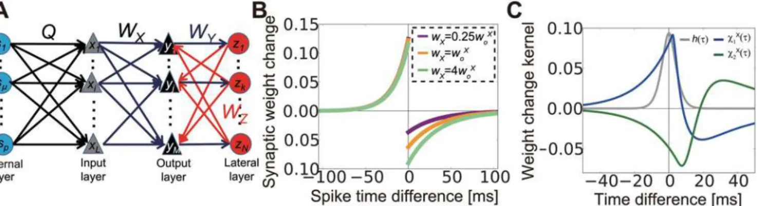
projects to the output layer, which also receives inhibitory feedback from the lateral layer. Neu-rons in the lateral layers are excited by inputs from the output layer. We assumed that all neu-rons in the input layer and the output layer are excitatory, whereas lateral-layer neuneu-rons are assumed to be inhibitory. Although excitatory lateral interactions also exist in the sensory cor-tex, they are typically sparse [30] and weak [10] compared with inhibitory interactions; thus we concentrated on the latter. For the analytical treatment, the neurons in the output and lateral layers were modeled with a linear Poisson model. We first studied synaptic plasticity at the feed-forward connections (connections from the input layer to the output layer), while fixing lateral connections (i.e., connections from the output layer to the lateral layer and connections from the lateral layer to the output layer). For STDP, we used pairwise log-STDP (Fig 1B) [31], which replicates the experimentally observed long-tailed synaptic weight distribution [32,33].
We considered the case for information encoded in the correlated activity of input neurons [34,35], and fixed the average firing rate of all input neurons at the constant valueυoX(See
Table1and2for the list of variables and parameters). If the firing rate of input neuroniis given as ro
i þ
X
p
m¼1
qim
ð1
0 ðt0Þs
mðtt0Þdt0, for external eventsμ(t)and the response probability
of the neuronqiμ, then common inputs from the external layer induce a temporal correlation
proportional to
hðt;ytÞ
ð1
maxðt;0Þ
dt0ðt0Þðt0tÞ: ð1Þ
whereφ(t)is a response kernel (see Eqs (14) and (24) in Methods for details). If we use
ðtÞ ¼t2et=yt=2y
t3, whereθtis the parameter that controls the timescale of spike correlations,
thenhðt;ytÞ ¼ 1 16yt3ðt
2þ3y
tjtj þ3yt
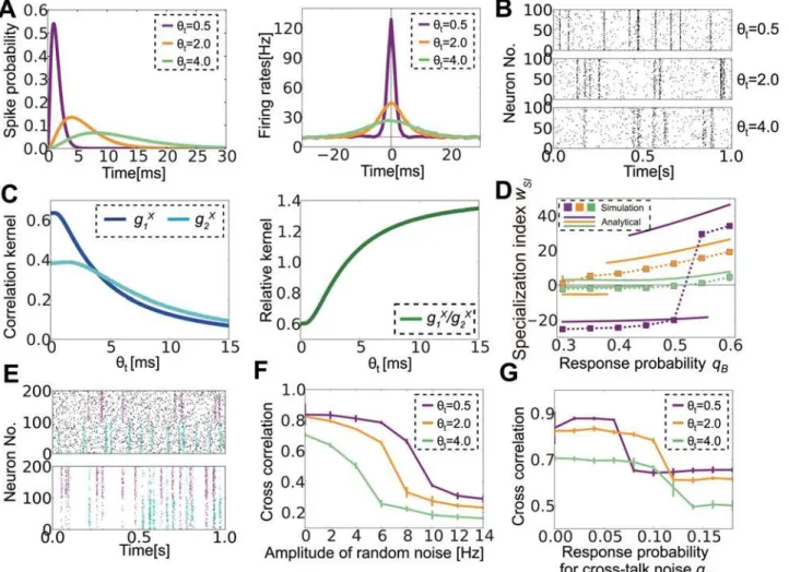
2Þejtj=yt(gray line inFig 1C). For the kernel function, we Fig 1. Description of the model.(A) Schematic figure of the model. (B) Spike-time dependent synaptic weight change in log- spike-timing-dependent plasticity (STDP). (C) Normalized temporal cross-correlogram of input neurons receiving common sources (gray line), and kernel functions of plasticity propagated by feedforward correlation (blue line) and feedback correlation (green line).
used the gamma distribution with shape parameterkg= 3 in order to reproduce broad spike
correlations typically observed in cortical neurons [36,37]. Synaptic weight dynamics by STDP is written as
dwX ji
dt ¼xiðtd Xa ji Þ
ð1
0
Fdðw X
ji;sÞyjðtsd Xd
ji Þdsþyjðtd Xd ji Þ
ð1
0
Fpðw X
ji;sÞxiðtsd Xa ji Þds
forFdðwXij;sÞ ¼fdðwXijÞe s=t
d,F
pðwXij;sÞ ¼fpðwXijÞe s=tp
, wherefd(w) andfp(w) are synaptic weight
dependence of LTD/LTP (long-term depression/potentiation), respectively. By taking the aver-age of above equation over time and ensemble (see Averaver-age synaptic weight velocity in Meth-odsfor details), the weight change of the feedforward connectionWXcan be approximated as
WX
WXðg X
1Eg
X
2WZWYÞC
t; ð2Þ
Cil(s) Cross correlation between input neuroniandl Eq (24) G1X(w),G2X(w) Coefficients of correlation-based synaptic weight change Eq (30)
χ1X,χ2X The correlation kernel functions Eqs (3) and (4) doi:10.1371/journal.pcbi.1004227.t001
Table 2. Parameter settings.
T Simulation time 3000 s (for Figs5C,5D,5E,6and7: T = 4000 s)
L,M,N Neural population 400, 20, 20 (for Figs7and8: M = N = 40) La,Ma,Na Neural subpopulation 100, 10, 10
τAX,τBX,τAY,τBY,τAZ, τBZ
EPSP/IPSP time constants 5.0, 1.0, 4.0, 0.8, 2.5, 0.5 ms
woX,woY,woZ Synaptic weights 2.5, 100.0, 50.0 (for Figs7and8:woZ= 80.0) dXamin,dXamax Axonal delays 2.0, 4.0 ms
dXdmin,dXdmax Dendritic delays 0.5, 1.5 ms
dY
min,dYmax,dZmin,
dZ max
Synaptic (axonal) delays 0.2, 1.2, 0.2, 1.2 ms
θt Correlation timescale 2.0 ms
νoS,νoX Firing rates 10, 10 Hz
ηX Learning rate 0.05woX
σsig Noise amplitude of plasticity 0.3
τp,τd STDP time windows 17, 34 ms
α,β Parameters for log-STDP 20.0, 50.0
σWinit Initial variance of synaptic
weights
0.1
γY,γZ LTD/LTP balance 1.4, 0.7
where g1Xand g2Xare scalar coefficients,Cis the correlation matrix, andEis the identity
ma-trix (see Eqs (25)–(30) for derivation). Thefirst term describes the synaptic weight change di-rectly caused by an input spike correlation and can be rewritten into the convolution of the temporal correlation and correlation kernel functionχX1as
gX
1 G
X
1ðw
X oÞ;G
X
1ðwÞ
ð1
1 wX
1ðt;wÞhðtÞdt;
wX
1ðt;wÞ ¼
ð1
tþ2dXd
dsFðw;sÞ"Xðtþs2dXdÞ; ð3Þ
whereF(w,s) =Fd(w,-s) ifs<0, elseF(w,s) =Fp(w,s), and"Xis the EPSP curve of input neurons
(see Eqs (15) and (31) in the Methods). By the deconvolution ofG1X(w), we can separate the
ef-fect of the intrinsic network propertyχX1and that of the input correlationh(τ)for STDP-based
learning. Due to causality, LTP/LTD balance, and dendritic delay,wX
1ðt;wÞtypically becomes
LTP-dominant aroundτ= 0 (blue line inFig 1C; we setw=woX), so thatg1Xtakes positive
val-ues, which enables coincidence-based learning [4,5,38]. The second term ofEq (2), which is of particular interest in this model, describes how the input correlation influences STDP learning at feedforward connections through lateral inhibition:
gX
2 G
X
2ðw
X oÞ;G
X
2ðwÞ
ð1
1 wX
2ðt;wÞhðtÞdt;
wX
2ðt;wÞ ¼
ð1
tþD
dsFðw;sÞ
ðtþsD
0
dr"ZðrÞ
ðtþsrD
0
dq"YðqÞ"XðtþsrqDÞ; ð4Þ
whereD= 2dXd+dY+dZ, and"Yand"Zare EPSP/IPSP curves of output/inhibitory neurons,
respectively. This term primarily causes LTD as the signflips through lateral inhibition (wX
2ðt;wÞ; shown as the green line inFig 1C). Previous simulation studies showed lateral
inhi-bition has critical effects on excitatory STDP learning [17–19]; however, it has not yet been well studied how a secondary correlation generated through the lateral circuits influences STDP at feedforward connections, and it is still largely unknown how lateral inhibition func-tions with various stimuli in different neural circuits. For example, the correlation kernel of the feedback term exhibits a delay as the signal propagates through the inhibitory circuit; yet, we do not know how much delay is permitted for effective learning or if realistic synaptic delays satisfy such a condition. Furthermore, it is also unknown what information a circuit can learn if there are several mixed signals with different amplitudes for which symmetry-breaking learn-ing [5,39] is not valid. Therefore, using theoretical analysis and simulation, wefirst investigated the properties of the inhibitory kernelwX
2ðt;wÞin STDP learning.
Lateral inhibition enhances minor source detection by STDP
InEq (2), if lateral inhibition is negligible (i.e.,g2X/g1X= 0), all output neurons acquire the
(cA= 0.36) than those receiving the output of source B (cB= 0.25). In the matrix form,
Q¼
qA 0
0 qB
0 0
0
B @
1
C A;C¼
cA 0 0
0 cB 0
0 0 0
0
B @
1
C A:
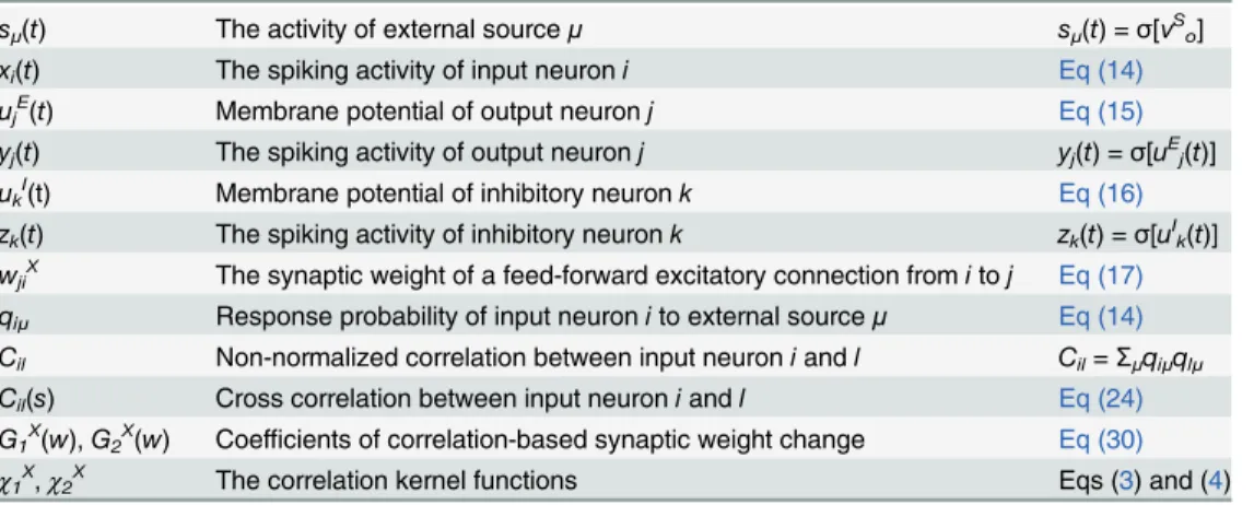
Fig 2. Lateral inhibition enables minor source detection by spike-timing-dependent plasticity (STDP) through membrane hyperpolarization.(A) Schematic figure of the simplified model. SAand SB(on the left side) are the sources that project to subsets of input neurons (colored triangles). Gray
triangles are background neurons, black triangles (on the right) are output neurons, and red circles are inhibitory neurons. (B) Development of synaptic weights. Thick lines are mean synaptic weights from A-neurons (blue), B-neurons (red), and Background-neurons (orange) to each output neuron. Thin lines are traces of individual synaptic weights. Gray bar shows the timing at which figure C is calculated. (C) Peristimulus time histograms (PSTHs) of membrane potentials averaged within output neuron groups. T = 0 indicates the timing of events at external layers. The three figures are calculated from the data at t = 0–1 min, 7–8 min, and 29–30 min. (D) Development of mean cross-correlation and mutual information between external sources and population activity of output neurons for the simulation depicted in panels B and C. (E) Delay dependence of mean cross-correlation and mutual information. Both values were calculated from five simulations. (F) Cross-correlation between the output group that detected the minor source and the minor source activity for various response probabilitiesqBwith a fixedqA(= 0.6). When none of output groups detected the minor source, the larger value calculated for the two output groups
was used. Throughout the study, error bars represent standard deviation calculated from five simulations, unless otherwise indicated.
The third row in Q represents response probabilities of background neurons in the input layer (gray triangles inFig 2A; note that C = QQt). We refer to this as the minor source detection task below. Here, for lateral connections, we assumed that both excitatory-to-inhibitory (E-to-I) and inhibitory-to-excitatory (I-to-E) connections are well organized such that inhibi-tion only works mutually between two output neuron groups (Fig 2A; blue lines are E-to-I and red lines are I-to-E connections. See alsoEq (30)in Methods). The origin of these structured lateral connections is discussed later. When the network is excited by inputs from external sources, excitatory postsynaptic potential (EPSP) sizes of feedforward connectionsWXchange
according to STDP rules. Initially, in all output neurons, synaptic weights from A-neurons (blue triangles inFig 2A) become larger because A-neurons are more strongly correlated with one another than B-neurons are. However, as learning proceeds, one of the output neuron groups becomes selective for the minor source B (Fig 2B). After 30 min, the network successful-ly learns both sources. If we focus on the peristimulus time histogram (PSTH) for the average membrane potential of output neurons aligned to external events, both neuron groups initially show weak responses to both correlation events, and yet the depolarization is relatively higher for source A than for source B (Fig 2Cleft). After 10 min of learning, both neuron groups show relatively stronger initial responses for source A, but group 1 shows a hyperpolarization soon after the initial response (Fig 2Cmiddle). As a result, synaptic weights from A-neurons to group 1 become weaker, and group 1 neurons eventually become selective for the minor source B (Fig 2Cright). The mean cross-correlation (see cross-correlation inMethodsfor details) be-tween the external sources and the population activity of output neurons is maximized when the delay is approximately 10–15 ms (Fig 2E). If wefix the delay at 14 ms, then the cross-correlation gradually increases as the network learns both sources (Fig 2D). The same argu-ment holds if mutual information is used for performance evaluation (green lines in Fig2D and2E). Interestingly, the network better detects the minor source when it is learned with a highly correlated source compared with when it is learned with another minor source (Fig 2F), because a highly correlated opponent source causes strong lateral inhibition on the output neu-rons, which enhances minor source learning. Similar results are also obtained for conductance-based leaky integrate-and-fire (LIF) neurons (S1 Fig).
Lateral inhibition should be strong, fast, and sharp
To investigate how and when the network can acquire multiple sources represented by corre-lated inputs, we further analyzed the model above (see Mean-field approximation of a two-source model inMethodsfor details). Because both output excitatory neurons and lateral inhibitory neurons are bundled into groups, in the mean-field approximation, we can approxi-mate M excitatory populations and N inhibitory populations into two representative output neurons and two inhibitory neurons. Similarly, input neurons can be bundled into three groups (A-neurons, B-neurons, and Background-neurons). In addition, we assumed that the synaptic connections from Background-neurons to output neurons are fixed because they showed little weight change in the simulation (orange lines inFig 2B). In this approximation, by inserting Eq (32)intoEq (29), the mean synaptic weight changes of feedforward connections follow
dwX mn
dt ffi X
L=La
n0¼1
Law X mn0nSoG
X
1ðw
X mnÞ
X
r
qnrqn0rNawZMawY
X
L=La
n0¼1
Law X mn0nSoG
X
2ðw
X mnÞ
X
r
qnrqn0r
þFðwX mnÞ ðnXoÞ
2XL
=La
n0¼1
Law X mn0 ðnXoÞ
2
NawZMawY
XL =La
n0¼1
Law X
mn0þ ðNawZÞ 2
MawYnXonZm
" #
;
ð5Þ
learning, and the last term is the homeostatic effect intrinsic to STDP [5].G1XandG2Xare
coef-ficients determined by synaptic delays, EPSP/IPSP (Inhibitory postsynaptic potential) shapes, and correlation structure, as shown in Eqs (3) and (4). By solving the self-consistency condition (Eq (34)in Methods), thefiring rates of inhibitory neurons are approximated as
nZ
1¼
MawYnXo 1 ðMawYNawZÞ
2 ðLaw1AþLaw1Bþ2Law
X
oÞ ðMawYNawZÞðLaw2AþLaw2Bþ2Law X oÞ
nZ
2¼
MawYnXo 1 ðMawYNawZÞ
2 ðLaw2AþLaw2Bþ2LawXoÞ ðMawYNawZÞðLaw1AþLaw1Bþ2LawXoÞ
:
ð6Þ
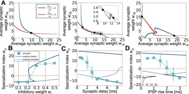
We estimated the nullclines by calculating the lines that satisfy
_
w1mðw1A;w1B;w2Aðw1A;w1BÞ;w2Bðw1A;w1BÞÞ ¼0 forμ=AorB. As a result, we found that when
the mutual inhibition is weak (wI= 10), the system has only one stable point at whichw1Ais
larger thanw1B(Fig 3Aleft). At this point,w2Ais also larger thanw2B(w2A= 9.64,w2B= 3.60;
not shown in thefigure), which means that both output neuron groups are specialized for the major source A (we call this state a winner-take-all state or T-state); however, if the inhibition is moderately strong (wI= 21.5), two new stablefixed points and two unstablefixed points
ap-pear in the system (Fig 3Amiddle). In the stable point on the left, neuron group 1 picks up source B while neuron group 2 picks up source A (w2A= 12.52,w2B= 2.87). On the right-hand
side, neuron group 1 selects source A while neuron group 2 selects source B (we denote those two states as winners-share-all states or S-states below). At the stable point in the middle, both groups detect source A (w1A=w2A= 9.47,w1B=w2B= 3.61). Note that because of the mutual
Fig 3. Lateral inhibition is strong, fast, and sharp.(A) Nullclines of the average synaptic weight changes at different inhibitory amplitudeswZ= 0.1, 0.215,
0.4. The inset in the middle graph is a magnified view of boxed area. (B) Specialization indiceswSIfor various inhibitory weights. PositivewSIindicates the
winner-share-all state, whereas negativewSIindicates the winner-take-all state. Blue lines are analytical estimations and cyan squares are the results of
simulations. Vertical lines correspond to the values at which the nullclines in Figure A are calculated. (C) The same graphs for various synaptic delays. The average synaptic delay of both lateral excitatory (dY
min+dYmax)/2 and inhibitory (dZmin+dZmax)/2 connections was changed, while the variability was kept at dY
max—dY
min=dZmax—dZmin= 1.0 ms. (D) IPSP rise time dependence. The inset shows IPSP curves at {τZA,τZB} = {0.5, 2.5} (gray line), {1.5, 7.5} (dark gray
line), and {2.5, 12.5} (black line).
inhibition, the synaptic weight from A-neuron is smaller when both groups learn A than it is when only group 1 learns A. For strong inhibition (wI= 40.0), the stable point in the middle
disappears, and the system is stable only when two neuron groups detect different sources (Fig 3Aright). Simulation results confirm this analysis because strong inhibition indeed causes a winner-share-all state in which multiple neuron groups survive in competition [15], whereas the network tends to show a winner-take-all learning when the inhibition is weak (Fig 3B). We measured the degree of winner-share-all/winner-take-all states by defining the specialization indexwSIas
w0
SI¼ ðw1Aw1BÞðw2Bw2AÞ;wSI¼w0SI=
ffiffiffiffiffiffiffiffiffiffi
jw0 SIj
p
: ð7Þ
Ifw’SI= 0, we setwSI= 0. If two output groups are specialized for different sources,wSIbecomes
positive, whereas if two groups are specialized for the same source,wSIbecomes negative.
When the synaptic delay in the lateral connections is small, only S-states are stable, whereas at longer delays, both S-states and T-states are stable. In the simulation, the network typically grows toward the latter state in the bistable strategy (Fig 3C). Moreover, if we change the shape of the IPSP curve while keepingτZB= 5τZA, for steep IPSP curves (i.e., bothτZAandτZBare
small), only the S-states are stable, whereas T-states also become stable for slower IPSPs (Fig 3D). Therefore, both analytical and simulation studies indicate that lateral inhibition should be strong, fast and sharp to detect higher correlation structure. Moreover, lateral inhibition does not need to be pathologically strong because the I/E balance ofNawZ=LwXo ffi20% is sufficient
to cause multistability.
Optimal correlation timescale changes depend on the noise source
In the previous section, we revealed the effects of network properties for a fixed input correla-tion structure; however, actual neurons show various timescales for correlacorrela-tions depending on the brain region [37,42] and characteristics of the stimuli [43,44], and it is largely unknown how different timescales influence correlation-driven learning. Therefore, we next considered the effect of correlation timescales, especially on noise tolerance. In our current model, input neurons respond to external sources with input kernelðtÞ ¼t2et=yt=2yt
3(Fig 4Aleft), and so
the correlation between input neuroniandlis given as
CilðsÞ ¼n S o
X
p
m¼1
qimqlmhðsÞ:
By changing the parameterθt, we studied the effect of the correlation timescale on learning.
The correlation is precise whenθtis small, whereas it becomes broad at large values ofθt(Fig
4Aright,Fig 4B). Because STDP causes homeostatic plasticity that does not depend on a corre-lation, as shown in the third term ofEq (5), in a more precise approximation,Eq (2)should be written as
WX
WXðg X
1Eg
X
2WZWYÞC
t
þ hhomeostatic termi: ð8Þ
Wefirst calculatedg1Xandg2Xat variousθt. Bothg1Xandg2Xbecome smaller for a largerθt,
but decreases ing2Xare slower than those ing1X, and, as a result,κ=g2X/g1Xbecomes larger for
a longer correlation timescale (Fig 4C). This means that a longer temporal correlation is more suitable for the detection of multi-components. This is indeed confirmed in the simulation (Fig 4D). Whenθt= 0.5 and the minor component is slightly weaker than the major one (cA= 0.36,
cB= 0.25), the minor component is no longer detectable. On the other hand, atθt= 2.0, the
(cA= 0.36,cB= 0.16). Atθt= 4.0,g1Xbecomes smaller so that even the major signal is not
fully detectable.
Similar results hold for crosstalk noise. In the model above, the noise is provided through the spontaneous Poisson firing of input neurons as random noise (Fig 4Etop, black dots are spikes caused by random noise). In reality, however, there would be crosstalk noise among input spike trains caused by the interference of external sources. We implemented this cross-talk noise by introducing non-diagonal components in the response probability matrix as
Q¼
qS qN
qN qS
0 0
0
B @
1
C A;
Fig 4. Optimal correlation timescale changes depending on noise characteristics.(A) Response kernels of input neurons to external events (left) and cross-correlation among input neurons responding to the same source calculated from simulated data (right) for three different correlation timescale parametersθt. (B) Raster plots of input neurons for variousθt. Only 100 correlated neurons are plotted although there are 400 input neurons in total. (C)
Analytically calculated correlation kernelsg1X,g2X(left), and their ratiog1X/g2X. (D) Specialization indexwSIfor various response probabilitiesqBwhile fixing qA= 0.6. Lines representwRat analytically estimated stable points, and dotted squares represent simulation results. (E) Raster plots of two types of noise.
The upper panel shows random noise, whereas the lower panel depicts crosstalk noise. In both panels, the first 100 neurons respond primarily to the cyan source, and the next 100 neurons respond to the purple source. For random noise, the noise (black dots) is independent from the signals, whereas the crosstalk noise (purple dots in the lower half, cyan dots in the upper half) is correlated with the signal for the other population. (F, G) The effects of random noise (F) and crosstalk noise (G) at various correlation timescales.
whereqSis the response probability to the preferred signal andqNis that to the non-preferred
signal (Fig 4Ebottom). We refer to this as the noisy source detection task below. To make a clear comparison, in the simulation of random noise, we keptqN= 0 and changed the
sponta-neousfiring rate of the input neurons (rio) to modify the noise intensity, whereas in simulation
of crosstalk noise we removed random noise (i.e.,rio= 0) and changedqN. For random noise, a
smallerθtenables better learning because a largeg1Xcompetes with the homeostatic force (Fig
4F). By contrast, for crosstalk noise, the performance is better atθt= 2.0 than atθt= 0.5 because
strong lateral inhibition suppresses crosstalk noise (Fig 4G). Although for small noise regi-mens, the network performs better atθt= 0.5 than atθt= 2.0, but the difference is almost
negli-gible. Therefore, to cope with crosstalk noise, the spike correlation needs to be broad, whereas a narrow spike correlation is better for random noise. We note that qualitatively the same argu-ments as above also hold for the exponential kerneleðtÞ ¼et=yt=
yt(S3DandS3EFig). How-ever, the ratio of two coefficients (i.e.,κe=ge2X/ge1X) is typically smaller for this kernel than for
the kernel we used throughout this study (S3BandS3CFig vs.Fig 4D) because lateral inhibi-tion is less effective due to highly peaked spike correlainhibi-tion (S3A Fig).
Excitatory and inhibitory STDP cooperatively shape structured lateral
connections
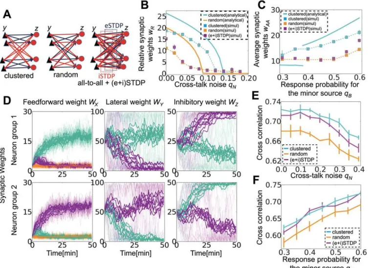
To this point, we have considered a network already clustered into two assemblies that inhibit one another (as inFig 5Aleft). This means that the network somehow knows a priori that the number of external sources is two; however, in reality, a randomly connected network should also learn such information. To test this idea, we introduced STDP-type synaptic plasticity in lateral excitatory connections and feedback inhibitory connections and investigated how differ-ent STDP rules cause differdiffer-ent structures in the circuit.
We first checked whether structured lateral connections were helpful for learning. For com-parison, we also considered a model with random lateral connections in which all output neu-rons and inhibitory neuneu-rons are randomly connected with probability 0.5 (Fig 5Amiddle). When lateral connections are random, mean-field equations are modified as
dwX mn
dt ffi X
L=La
n0¼1
Law X mn0nSoG
XðwX mnÞ
X
r
qnrqn0rNawZMawY
X
p
m0¼1
X
L=La
n0¼1
Law X m0n0nSoG
YðwX mnÞ
X
r
qnrqn0r
þFðwX mnÞ ðn
X oÞ
2XL
=La
n0¼1
Law X mn0 ðnXoÞ
2
NawZMawY
Xp
m0¼1
XL =La
n0¼1
Law X
m0n0þ ðNawZÞ 2
MawYn X on
Z tot
" #
;
nZ tot
2MawYnXoðLaw1AþLaw1Bþ2LawXoÞ 1þ2MawYNawZ
:
ð9Þ
We separated lateral connections into two groups as in the previous case, but this approxi-mation is legitimate only when two input sources are symmetrical (i.e.,qA=qB). In other cases,
neurons are often organized into two groups with different population sizes. In such cases, for evaluating performance, we measured average weights from source A on the output neurons receiving stronger inputs from A-neurons than from B-neurons or Background-neurons. For randomly connected lateral inhibition, learning performance dropped significantly in noisy source detection (Fig 5B) and in minor source detection (Fig 5C); thus clustered connectivity is indeed advantageous for learning.
learning is achievable only when the learning of a hidden external structure is possible from the random lateral connections (magenta lines in Fig5Band5C; note that orange points are hidden by magenta points because they show similar behaviors in noisy cases), which means ei-ther when crosstalk noise is low or two sources have similar amplitudes. Nevertheless, once a structure is obtained in easy settings (qN= 0 orqA=qB), that network outperforms the network
with random lateral connections in both noisy source detection (Fig 5E) and minor source de-tection (Fig 5F). InFig 5E, we evaluated the performance of noisy source detection by first con-ducting STDP learning atqN= 0, and then we terminated STDP and performed simulations at
the various noise levelsqN. Similarly, in the minor source detection task depicted inFig 5F, we
first performed STDP learning withqA=qB= 0.6, and then evaluated the performance for a
Fig 5. Lateral connection structuring by excitatory and inhibitory spike-timing-dependent plasticity (STDP).(A) Schematic figures of connections between the output layer and the lateral layer. In the simulation, each layer consists of 20 neurons. (B) The effect of crosstalk noise on different lateral structures. Analytical results are shown as bold lines, and the results from simulations are shown as dotted lines. (C) Minor source detection with different lateral structures. Because the specialization index is not well defined for a network with random lateral connections, the average synaptic weights from source A to those output neurons that prefer source A were measured instead. (D) Synaptic weight development at three connections. In the left and right columns, panels show synaptic weights of excitatory/inhibitory synapses projected to the neuron group 1 (top) and group 2 (bottom). In the middle graph, panels correspond to excitatory synapses projected from the neuron group 1 (top) and group 2 (bottom). In all panels, thin lines indicate the development of individual synapses, thick lines represent average weights onto output neurons, and colors indicate A-neurons (blue), B-neurons (red), and Background-neurons (orange). (E, F) Performance of the network with different lateral structures in noisy signal detection (E) and minor signal detection (F). Here (and only here), a pre-learned network is used to investigate responses for various inputs.
smallerqB. STDP can also generate similar lateral connection structures when the total number
of input sources is larger than two (S2AandS2BFig). Therefore, STDP at lateral connections helps signal detection by efficiently organizing the connection structure.
We next studied the analytical conditions for learning of the clustered structure (see Analyt-ic approach for STDP in lateral and inhibitory connections inMethodsfor details). The synap-tic weight dynamics of lateral excitatory and inhibitory connections are approximately given as
WY
gY
1WYWXCtWtX;g
Y
1
ð1
1
dsFY ðsÞ
ð DX r ð DY u ð DX
r0hðuþr0srÞ
WZ
gZ
1WXCWXtW
t Y;g
Z
1
ð1
1
dsFZ ðsÞ
ð DX r ð DY u ð DX
r0hðrsur0dZdYÞ: ð10Þ
Both equations represent indirect effects of the input correlation propagated into the lateral cir-cuit. From a linear analysis, we can expect that whengY1is positive, E-to-I connections tend to
be feature selective (seeEq (35)in Methods). Each inhibitory neuron receives stronger inputs from one of the output neuron groups and, as a result, shows a higherfiring rate for the corre-sponding external signal. On the other hand, ifgZ1is positive, I-to-E connections are organized
in reciprocal form, where one of the reciprocal connections is enhanced and the other is sup-pressed (seeEq (36)in Methods). We can evaluate feature selectivity of inhibitory neurons by
φY ¼ 1
N
X
Nk¼1 1
jOY Aj
X
j2OYA wY
kj 1
jOY Bj
X
j2OYB wY kj 0 B @ 1 C A
=
1 MX
Mj¼1
wY kj
0
@
1
A; ð11Þ
whereOYAandOYBare the sets of excitatory neurons responding preferentially to sources A
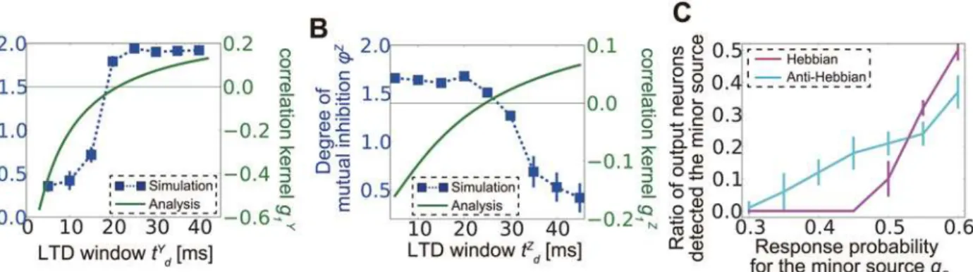
and B, respectively. Indeed, when the LTD time window is narrow, analytically calculatedgY1
tends to take negative values (the green line inFig 6A), and E-to-I connections organized in the simulation are not feature selective (the blue points inFig 6A). By contrast, for a long LTD time window (i.e., when LTD is weakly spike-timing dependent),gY1tends to take positive
val-ues, and E-to-I connections become clustered. In the simulation,WZis also plastic, but as
shown inEq (10), the effect ofWZon the plasticity ofWYis negligible infi
rst-order approximations.
Similarly, for I-to-E connections, we measure the degree of mutual inhibition (non-reciprocity) with
φZ ¼1
N XN
k¼1
wY kj
XM
j¼1
wY kj w Z jk XM
j¼1
wZ jk
: ð12Þ
When LTD is strongly spike-timing dependent,gZ1is negative andϕZcalculated from the
Hebbian inhibitory STDP at lateral connections is not always beneficial for learning. For ex-ample, in minor source detection, if we use Hebbian inhibitory STDP, a slightly minor source is not detectable, whereas for anti-Hebbian STDP, a small number of neurons still detect the minor source because reciprocal connections from strong-source responsive inhibitory neu-rons to strong-source responsive output neuneu-rons inhibit synaptic weight development for the stronger source (Fig 6C).
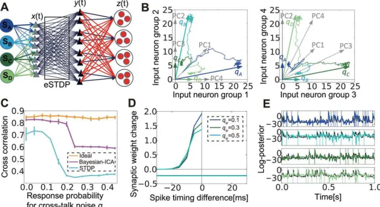
Neural Bayesian ICA and blind source separation
Our results to this point have revealed that correlation-based STDP learning combined with lateral inhibition can successfully detect signals from mixed inputs masked by noises. To con-firm this mechanism is indeed effective in realistic tasks, we applied the above method to blind source separation. We first examined the condition in which the network could capture exter-nal sources. We extended the previous network to include four independent sources mixed at the input layer (Fig 7A). In the present application, we used structured lateral connections be-cause learning for clustered structures is difficult with noisy stimuli, as shown in the preceding section. The response probability matrix Q and correlation matrix C are given as
Q¼
qS qN 0 qN
qN qS qN 0
0 qN qS qN
qN 0 qN qS
0
B B B B @
1
C C C C A
;C¼
qS2þ2qN2 2qSqN 2qN2 2qSqN
2qSqN qS
2þ2q
N
2 2q
SqN 2qN
2
2qN
2 2q
SqN qS 2
þ2qN
2 2q
SqN 2qSqN 2qN
2 2q
SqN qS
2þ2q
N 2
0
B B B B @
1
C C C C A
:
Therefore, the principal components of matrix Q (i.e., eigenvectors of C) are {1, 1, 1, 1,}, {-1, 0, 1, 0}, {0, -1, 0, 1}, {-1, 1, -1, 1}. Because thefirst-order approximation of synaptic weight dy-namics followsWX
gX
1WXCt, we may expect that synaptic weight vectors converge to the
ei-genvectors of the principal components; however, this was not the case in our simulations, even if we took into account the non-negativity of synaptic weights (seeFig 7B, where we renormalized the principal vectors to the region between 0 and 1). Instead, each weight vector converged to a column of the response probability matrix Q (Fig 7B, the left panel is the projec-tion to thefirst two dimensions, and the right panel is the projection to the other two
Fig 6. Correlation propagation shapes lateral connection structure.(A) Comparison between feature selectivityϕY(blue dots) calculated from simulation results and analytically calculated correlation kernel functiong1Y(green line) for lateral excitatory connections. Thin green horizontal line representsg1Y= 0.
(B) Comparison between the degree of mutual inhibitionϕY(blue dots) calculated from the simulation and analytically calculated correlation kernel g1Z(green line) for lateral inhibitory connections. Negativeg1Zis correlated with a high degree of mutual inhibition, as expected (seeMethods). (C) Ratio of
output neurons tuned for the minor source in a minor source detection task under Hebbian and anti-Hebbian inhibitory spike-timing-dependent plasticity.
dimensions). This result implies that the network can extract independent sources, rather than principal components, from multiple intermixed inputs.
We next evaluated the performance of hidden external source detection, especially its toler-ance against crosstalk noise. To this end, we compared the performtoler-ance of the model with that of the Bayesian ICA algorithm, in which independence of external sources is treated as a prior [46,47]. In the algorithm, the learned mixing matrix may converge to its Bayesian optimal value estimated from a stream of inputs. Although we cannot directly argue the optimality of cross-correlations, if the mixing matrix is accurately estimated, external activity is also well in-ferred, and thus we can use the mean cross-correlation as a measure for the optimality of learn-ing. In terms of discretized input activityX, the external source activitySand prior
informationI, we can express the conditional probability of the estimated response probability
matrixQ~asP½Q~jX;I ¼P½Q~jI
P½XjI
ð
P½XjS;Q~;IP½SjIdS(see Bayesian ICA inMethodsfor
de-tails). This means that even if no prior information is given forQ~itself (i.e.P½Q~jI ¼const:),
posteriorP½Q~jX;Istill depends on a prior given forS. If we introduce a prior that each
exter-nal source follows an independent Bernoulli Process
(i.e.P½SjI ¼Y T=Dt
k¼1
YL
i¼1
ðrsDtÞskmð1r
sDtÞ1skm), then the stochastic gradient descendent of posterior Fig 7. With lateral inhibition, spike-timing-dependent plasticity (STDP) mimics Bayesian independent component analysis (ICA).(A) Schematic figure of the model with four sources. (B) Synaptic weight development in input neuron space. ArrowsqAtoqDare response probability vectors of the four
sources, and PC1 to PC4 are normalized principal components of the correlation matrix C. Lines represent traces of average synaptic weight from each input group to the output groups that learned corresponding sources during the learning process. (C) Comparison of performance among the ideal observer, Bayesian ICA learning, and STDP learning. (D) LTP/LTD time window of Bayesian ICA learning. (E) Behaviors of log-membrane potential (color lines) in the STDP model, and estimated log-posterior (black lines) in the Bayesian ICA algorithm for the same stimuli. Vertical lines represent timings of external events. Log-membrane potentials are normalized to align the mean and the variance to the corresponding log-posteriors.
We approximated this Bayesian ICA algorithm by a sequential sampling source activity in-stead of calculating the integral over all possible combinations in the estimation of the log-pos-terior of the response probability matrix Q. In this approximation, the learning rule of the estimated response probability matrixQ~obeys
D~qk im/
2xk i 1
xk
ipkiðY1:k1Þ=ð1pkiðY1:k1ÞÞ þ ð1xkiÞ
X1 k0¼0k0y
kk0 m
1~qk im
X1
k0¼0k0y kk0 m
pk iðY
1:k1Þ ¼1 1ro
iDt
Y
p
m¼1
1~qk im
X1
k0¼0 k0ykk
0 m
" #
; ð13Þ
where Y is the sampled sequence, andpik(Y1:k-1) is the sample based approximation of pikin
the previous equation. This rule has spike-timing and weight dependence similar to those seen in STDP (Fig 7D). Although the performance of STDP is much worse than the ideal case (when the true Q is given), this performance is similar to that for the sample-based learning al-gorithm discussed above (Fig 7C). Therefore, the network detects independent sources if cross-talk noise is not large. We further studied the response of the models for the same inputs and
found that the logarithm of the average membrane potentialuE
m¼
1
jOmj
X
j2Om uE
j well
approxi-mates the log-posterior estimated in Bayesian ICA, even in the absence of a stimulus (Fig 7E). This result suggests that in the STDP model, expected external states are naturally sampled through membrane dynamics that are generated through the interplay of feedforward and feedback inputs.
We finally performed the blind separation task using the same network as shown inFig 7A. We created“sensory”inputs by mixing four artificially created auditory sequences (Fig 8Aand S1 Auditory File). In the auditory cortex, various frequency components of a sound, particular-ly high-frequency components, are represented by specific neurons typicalparticular-ly organized in a tonotopic map structure [48], whereas low-frequency components are expected to be perceived as a change in sound pressure. Furthermore, populations of neurons in the primary auditory cortex are known to synchronize the relative timing of their spikes during auditory stimuli and provide correlated spike inputs for higher cortical areas in which the auditory scene is fully an-alyzed and perceived [49,50]. We modeled these features by assuming that input neurons have a preferred frequency {fi} defined as
fi¼exp
i
LðlogfmaxlogfminÞ þlogfmin
;
and auditory inputs are provided as time-dependent response probabilities, which follow qiðtÞ ¼qo
X
q
aqlðtÞa q
hðfiÞ, wherea q
Fig 8C), andaql(t) is the temporal change of the sound pressure (black lines inFig 8B). In this
representation, each sound source is represented by correlated spikes of neural populations (right panel ofFig 8C). Even if signals have overlapping frequency components {aqh(f)}q, blind
separation is possible as long as {aql(t)}qare independent and have sharp rising profiles suffi
-cient to cause spike correlations. After learning, four output neuron groups successfully de-tected changes in the sound pressure of the four original auditory signals (colored lines inFig 8B) by correctly identifying the input neurons that encoded the signals. Therefore, STDP rules implemented in a feedforward neural network with lateral inhibition serve as a spike-based so-lution to the blind source separation or cocktail party effect problem.
Discussion
By analytically investigating the propagation of input correlations through feedback circuits, we revealed how lateral inhibition influenced plasticity at feedforward connections. We showed that a population of neurons could learn multiple signals with different strengths or mixed lev-els. In addition, we found that to perform learning from signals corrupted with random noise, the timescale of the input correlations needed to be in the range of milliseconds, whereas the timescale was broader for crosstalk noise, which may explain why the spike correlation of corti-cal neurons often exhibits a large jitter (approximately 10 ms) [36,37]. We also investigated the functional roles of STDP at lateral excitatory and inhibitory connections to demonstrate that
Fig 8. Blind source separation by spike-timing-dependent plasticity (STDP).(A) Four original auditory signals (from the top to the fourth set of signals) and one mixed signal (bottom). (B) Amplitudes of original signals (black lines) and those estimated from output firing rates (colored lines). (C) Spectra of auditory sourcesaq
h(f) (left). Raster plots of input neuron activity. Colors were probabilistically assigned based on expected sources. All figures were
calculated from the 30’00”–30’10”portion of the auditory signals and simulation.
Simultaneously recorded neurons in close proximity often show correlated spiking, yet the pre-cision of these correlations varies across brain regions. Neurons in the lateral geniculate nucle-us show strong spike correlations [42,51], while correlations in V1 [36,52] or higher visual areas [37] are less precise. Our results indicate the interesting possibility that these differences may reflect the different characteristics of the noise with which the various cortical areas need to contend. At an early stage of sensory processing, the major noise component may be en-vironmentally produced background noise from various sources; thus precise spike correlation is beneficial at this stage for noise reduction during signal detection and learning (Fig 4G). By contrast, in higher sensory cortices, crosstalk noise accumulated through signal propagation in circuits may form the primary noise source, so less precise spike correlation is preferable (Fig 4H). It would be intriguing to examine whether lower and higher cortical areas similarly change the strength of spike correlations for other sensory modalities.
STDP in E-to-I and I-to-E connections
It is known that both glutaminergic synapses on inhibitory neurons [53,54] and GABAergic synapses on excitatory neurons [55,56] show STDP, and it is also known that STDP at E-to-I connections plays an important role in developmental plasticity [57]; however, detailed proper-ties of these plasticiproper-ties are still largely disputable [58,59] and, reportedly, highly dependent on inhibitory cell type [60], neuromodulator [61], and region [58]. We showed that in a feedback circuit, Hebbian inhibitory STDP preferred winner-take-all while anti-Hebbian inhibitory STDP tended to cause winner-share-all (see Fukai and Tanaka 1997 for winner-share-all) at ex-citatory neurons (Fig 6D). This result indicates that different inhibitory STDP imposes differ-ent functions for excitatory STDP, which suggests that a neural circuit may select optimal inhibitory STDP for a specific purpose or strategy of learning, and this may differ across re-gions and be modified by neuromodulators. A recent study showed that inhibitory plasticity even directly influences the plasticity at excitatory synapses of the postsynaptic neuron [62]. In such cases, algorithm selection would play a more important role than it did for the standard STDP implemented in our model.
Once an adequate circuit structure is learned and inhibitory connections are organized into a feature-selective pattern, even if the input to the network becomes noisy or faint, the network can still robustly detect signals (Fig5Eand5F). This robustness would be useful for spatial learning, as contextual information is often uncertain.
STDP and Bayesian ICA
Our results indicated that STDP in a lateral inhibition circuit mimicked Bayesian ICA [46,47]. First, output neurons were able to detect hidden external sources, without capturing principal components (Fig 7B). Previous results suggest that for a single output neuron, an additional homeostatic competition mechanism is necessary to detect an independent component [7,22]. In addition, when information is coded by firing rate, homeostatic plasticity is critically impor-tant, because STDP itself does not mimic Bienenstock-Cooper-Munro learning [18]. However in our model, information was encoded by correlation, and mutual inhibition naturally in-duced intercellular competition so that intracellular competition through homeostatic plastici-ty was unnecessary. Moreover, our analytical results suggested the reason that independent sources are detected. To perform a principal components analysis using neural units, the syn-aptic weight change needs to follow
WX
¼WXCLT½WXCW t XWX;
where LT[] means lower triangle matrix [64,65]. This LT transformation protects principal components caused by the lateral modification from higher order components; however in our model, because all output neurons receive the same number of inhibitory inputsEq (2), all neu-rons are decorrelated with one another and develop into independent components.
Recently, it was shown that STDP can perform Bayesian optimal learning [66,67]. In the model used by those authors, the synaptic weight matrix is treated as a hyper parameter and es-timated by considering the maximum likelihood estimation of input spike trains. By contrast, in the Bayesian ICA framework, the mixing matrix (corresponding to synaptic weight matrix) is treated as a probabilistic variable. Using this framework, we needed to calculate an integral over all possible source activities in the past to derive stochastic gradient descendent; however, as shown inFig 7C, the stochastic learning was well performed by employing an approximation with sequential sampling. Moreover, we naturally derived an adequate LTP time window from the response kernel of input neurons to external events (Fig 7D). We also found that STDP self-organized a lateral circuit structure that performed better than a random global inhibition (Fig5Eand5F). Mathematically, to perform sampling from a probabilistic distribution, we first needed to calculate the occurrence probability of each state; however, in a neural model, membrane potentials of output neurons approximately represent the occurrence probability through membrane dynamics. In machine learning methods, integration over possible source activities is often approximated using Markov chain Monte Carlo (MCMC) sampling [68]. In-terestingly, a recent study showed that a recurrent network performed MCMC sampling [69,70], suggesting that our network may perform a more accurate sampling in the presence of recurrent excitatory connections.
Suboptimality of STDP
is harmful for computations and stable learning, the benefit of noise addition is highly limited, and the brain may recruit other mechanisms for near optimal learning.
Neural mechanism of blind source separation
Humans and nonhuman animals can detect a specific auditory sequence from a mixed, noisy auditory stimulus, a phenomenon often called the cocktail party effect. The mechanism under-lying the cocktail party effect remains elusive [26,28,29], although several solutions have been proposed [74,75]. An effective solution for this problem is ICA [76–78], and the neural imple-mentation of the algorithm has been studied by several authors [14,18,79,80]. Our study ex-tended these results through a rigorous analytical treatment on biologically plausible STDP learning of spiking neurons, and our analyses enabled us to discover interesting functions of correlation coding. Moreover, by explicitly modeling inhibitory neurons, we found that STDP at E-to-I and I-to-E connections cooperatively organized a lateral structure suitable for blind source separation. In addition, we successfully extended a previous model for the formation of static visual receptive fields [18,19] to a more dynamic model in an auditory blind source sepa-ration task. In realistic auditory scene analysis, the frequency spectrum of acoustic signals is first analyzed in the cochlea, where each frequency component is the mixture of sound compo-nents from independent sources. Compocompo-nents belonging to the same source may be separated and integrated by downstream auditory neurons for the perception of the original signal. These frequency components can be considered a mixed signal in the ICA problem [81]; thus even if signals are mixed in frequency space, if the amplitudes of the signals are temporally indepen-dent, blind separation is still achievable. In the neural implementation of the problem, if two frequencies are commonly activated in the same signal, neurons representing those frequencies show spike correlation under the presence of the signal; thus the learning process is naturally achieved by STDP learning. These results indicate an active role of spike correlation and STDP in efficient biological learning.
Methods
Model
Neural dynamics. Based on the previous study [7], we constructed a network model with one external layer and three layers of neurons (Fig 1A). The first layer is the external layer that corresponds to external stimuli or the sensory system’s response to these stimuli. For simplici-ty, we approximated the activity of external sources using a Poisson process with the constant rateνSo. If we define the Poisson process with raterass^ðrÞ, the activity of the external sourceμ
at timetis written assmðtÞ ¼s^ðn S
oÞ(seeTable 1for the list of variables). Neurons in the input
Poisson process, the spiking activity of the input neuronifollows
xiðtÞ ¼s^ r o i þ
Xp
m¼1
qim
ð1
0
ðt0Þsmðtt
0Þdt0
" #
; ð14Þ
whereriois the instantaneousfiring rate defined withrio¼n X
o
Xp
m¼1
qimn S
o,qiμis the response
probability for the hidden external sourceμ, andðtÞ ¼t2et=yt=2y
t
3is the response kernel for
each external event. In most theoretical studies, cross-correlations give an exponential decay or a delta function [5,38], but here we used a response kernel that produces broader correlations (Fig 4Aright), because the actual correlations observed in the cortex are usually not sharply peaked [36,37]. For instance, for the exponential kerneleðtÞ ¼et=
yt=y
t, correlations show a
peaked distribution even if the timescale parameterθtis several milliseconds (S3A Fig). Because
of the common inputs from the external layer, input neurons show highly correlated activity, which enables population coding of the hidden structure. Although here we explicitly assumed the presence of the external layer, these analytical results can also be applied for arbitrary reali-zation of a spatiotemporal correlation.
Output neurons are modeled with the Poisson neuron model [5,38,45] in which the mem-brane potential of neuronjat timetis described as
uE jðtÞ ¼
XM
i¼1
wX ji
ð1
0
"XðrÞxiðtrd X jiÞdr
XN
k¼1
wZ jk
ð1
0
"ZðrÞzkðtrd Z
jkÞdr; ð15Þ
wherewjiXandwjkZare the EPSPs/IPSPs of input currents from input neuronxiand lateral
neuronzk, respectively, convolution functions are defined as"XðrÞ ¼
er=tX Aer=t
X B
tX AtXB
and
"ZðrÞ ¼
er=tZAer=tZB
tZ AtZB
, and synaptic delays in the feedforward excitatory and feedback
inhibi-tory connections aredijXanddjkZ. For feedforward excitatory connections, the synaptic delay
dijXis given by the sum of the axonal delaydijaand dendritic delaydijd, whereas for inhibitory
connections, we assume for simplicity that the delay is purely axonal. The response of the out-put neuron followsyjðtÞ ¼s^½gEðuEjÞ. Similarly, inhibitory neurons in the lateral layer show
Poissonfiring based on the membrane potential {uIk}k= 1,. . .,Nwhich is defined as
uI kðtÞ ¼
XM
j¼1
wY kj
ð1
0
"YðrÞyjðtrd Y
kjÞdr; ð16Þ
for EPSPs of a lateral connectionwYkj, convolution function"YðrÞ ¼
er=tY Aer=t
Y B
tY AtYB
, and
synap-tic delay of the lateral connectiondYkj. The synaptic delay of the excitatory lateral connection is
also approximated as the axonal delay. The spiking activity of the inhibitory neurons is given withzkðtÞ ¼s^½gIðuIkÞ. For analytical tractability, we use a linear response curve gE(u) =uand
gI(u) =u.
Synaptic plasticity. For most of this study, we focused on synaptic plasticity in the feedfor-ward connectionWX, with fixed lateral synaptic weightsWYandWZ. When the timing of the
spikes at the cell bodies of pre- and postsynaptic neurons istpreandtpost, spike timings at the
synaptic sites arets
pre¼tpreþdajiandtposts ¼tpostþdjidwith axonal and dendritic delays ofd a
whereξis a Gaussian random variable. The log-weight dependence well replicates experimen-tally observed synaptic weight distributions [32,33] and is suggested to have an important func-tion in memory modulafunc-tion [82]. Analytical treatment below is applicable to other types of synaptic weight dependence, yet in the additive STDP (i.e.fp(w) =Cpandfd(w) =Cd), the
mean-field equation typically does not have any stablefixed point. In addition, under the mul-tiplicative STDP in which LTD has a linear rather than a logarithmic dependence on synaptic weight, strong correlation is often necessary to induce salient LTP [31]. The coefficientsCp= 1
andCd ¼CptXp=tXd are chosen so that total LTP and LTD are balanced around the referential
synaptic weight.
The STDP at E-to-I connections and I-to-E connections is similarly defined. For simplicity, we assume that synaptic delays are solely axonal (i.e.,dY
k;j¼d Y;a k;j,dkZ;j¼d
Z;a
k;j), and the change in
synaptic weight does not depend on the synaptic weight. To maintain the balance between LTP and LTD, coefficients are chosen asCY
p ¼1,C Y d ¼g
YCY pt
Y p=t
Y d ,Z
Y ¼0:3ZwY o=w
X
o. Similarly, for
I-to-E connections,CZ
p ¼1,CdZ¼gZCpZtZp=tZd ,ZZ¼0:3ZwZo=wXo. We also modify constant
(ini-tial) synaptic weights towoY= 50.0 andwoZ= 25.0, and bounded synaptic weights withwYmax
= 100.0 andwZmax= 50.0. In this normalization, the total lateral inhibition takes the same
value as that in the non-plastic model at the initial state. Time windows are defined asτpY=τdY
=τpZ=τdZ= 20.0 ms.
InFig 6C, anti-Hebbian STDP was calculated by
DwQ¼ Z
Qexp½ðts postt
s preÞ=t
Q
d ðif tposts >t s preÞ
ZQgQðtQ
d=tQpÞexp½ðt s pret
s postÞ=t
Q
p ðif t s post <t
s preÞ
(
for Q = Y or Z. Similarly, the correlation detector type of STDP inS2 Figwas defined as
DwQ ¼ Z
Qðexp½ðts
posttspreÞ=tQp ðtQp=t Q
dÞexp½ðtposts tspreÞ=t Q
dÞ ðif tposts >tpres Þ ZQgQðexp½ðts
posttpres Þ=tQp ðtQp=t Q
dÞexp½ðtposts tpres Þ=t Q
dÞ ðif tspost<tpres Þ
(
The anti-correlation detector was calculated by changing the sign of above equations.
Leaky Integrate-and-Fire (LIF) model. In the main text, we performed all simulations with a linear Poisson model for analytical purposes, although we also confirmed those results with a conductance-based LIF model (S1 Fig). In the LIF model, the membrane potentials of excitatory neurons follow
dvE j dt ¼ 1 tE m
ðvE
j VLÞ g EE j ðv
E
j VEÞ g EI j ðv
E j VIÞ;
dgEE j dt ¼ gEE j tEE s þ
X
Li¼1
wX ji
X
ts i
dðtts iÞ;and
dgEI j dt ¼ gEI j tEI s þ
X
Nk¼1
wZ jk
X
ts k
wheregjEEandgjEIare excitatory and inhibitory conductances, respectively, andtisandtksare
the spike timings of input neuroniand lateral neuronk. Similarly, for inhibitory neurons in the lateral layer,
dvI k
dt ¼
1
tI m
ðvI
kVLÞ g IE k ðv
I
kVEÞ g II kðv
I kVIÞ;
dgIE k
dt ¼ gIE
k tIE
s
þ
X
M
j¼1
wY kj
X
ts j
dðtts jÞ; and
dgII k
dt ¼ gII
k tII s
þwII
X
ts r
dðtts rÞ:
In addition to the excitatory inputs from the output layer, we added random inhibitory in-puts as Poisson processes with afixedfiring rateroIIfor inhibitory neurons. A neuronfires if
the membrane potential exceeds the thresholdVth, and immediately goes into a refractory
peri-od in which the membrane potential stays atVreffor 1 ms after spiking. Plasticity was
imple-mented forwjiXin the same manner as that for the Poisson model. Parameters were chosen as
VL= -70.0,VE= 0.0,VI= -80.0,Vref= -60.0,Vth= -50.0 mV,tmE= 20.0,tmI= 10.0,tsEE= 5.0,
tsEI= 2.5,tsIE= 4.0,tsII= 5.0 ms,woX= 0.001,woI= 0.008,woL= 1.0,roII= 1000.0 Hz,wIIo=
0.005,Cd= 1.8CpτpX/τdX, andα= 50.0. All other parameters were the same as those used in the
Poisson model (Table 2).
In the LIF model, synaptic weights develop in a manner similar to that for the linear Poisson model, although change occurs more rapidly (Fig 1B,S1A Fig). Both cross-correlation and mu-tual information behave as they do in the Poisson model, but the performance is slightly better, possibly because the dynamics are deterministic (Fig1Dand1E,S1BandS1CFig); however, membrane potentials show different responses for correlation events (S1D Fig) because output neurons are constantly in high-conductance states, so that correlation events immediately cause spikes. As a result, membrane potentials drop to theVref, and the average potential goes
down. Interestingly, after neuron groups detect different signals, a preferred signal initially causes hyperpolarization due to firing, but, subsequently, a non-preferred signal causes hyper-polarization due to lateral inhibition (Fig 1Dright). The PSTH of firing shows that the behavior of the membrane potential in the Poisson model is similar (Fig 1CandS1E Fig). This is natural, because in the linear Poisson model, the firing rate has linear relationship with the membrane potential, whereas in LIF model relationship between the average membrane potential and fir-ing rate is highly non-linear.
Bayesian ICA. If discretized withΔt, the time series of the external source activity is writ-ten asS¼ fsmkg
k¼1;:::;T=Dt
m¼1;:::;p , and input activity becomesX¼ fxikg k¼1;:::;T=Dt
i¼1;::;L . Therefore, for prior
in-formationI, the joint probability of sources S and the estimated response probability matrix Q is
P½S;Q~jX;I ¼P½XjS;Q~;IP½S;Q~jI=P½XjI:
Therefore, by considering marginal probability,
P½Q~jX;I ¼P½Q~jI
P½XjI
ð
P½XjS;Q~;IP½SjIdS: ð19Þ
Therefore, log-likelihood becomes
logP½Q~jX;I ¼log ð
dSY
T=Dt
k¼1
YL
i¼1
ðxk ip
k
iþ ð1x k iÞð1p
k iÞÞ
Y
p
m¼1
ðrsDtÞskm
ð1rsDtÞ1skm
" #!
: ð20Þ
By taking gradient descendent,
@ @~qim
logP½Q~jX;I ¼1
Zp
X
T=Dt
k¼1
ð
P½S;XjQ~;I 2xki1
xk
ipki=ð1pkiÞ þ ð1xkiÞ
X1 k0¼0k0s
kk0 m
1~qim
X1
k0¼0k0s kk0 m
dS:
Therefore, we need to calculate the integral over all possible combinations of sources in the past to obtain stochastic gradient descendent; however, such a calculation is computationally difficult and incompatible with neural computation. Instead, we used sequential sampling of Y¼ fymkg
k¼1;:::;T=Dt
m¼1;:::;p , which is randomly sampled from
P½yk¼sk /P½sk;xkjY1:k1;Q~;I
¼Y
L
i¼1
ðxk ip
k iðs
k;Y1:k1
Þ þ ð1xk iÞð1p
k iðs
k;Y1:k1
ÞÞÞ Y p
m¼1
ðrsDtÞymk
ð1rsDtÞ1ykm; ð21Þ
where
pk iðy
k;Y1:k1
Þ ¼1 ð1ro iDtÞ
Y
p
m¼1
1~qim
X1
k0¼0 k0ykk
0 m
" #
:
Note in the above equations,xkis given as afixed value and not a random variable. Under this sample-based approximation, the stochastic gradient descendent follows
Dq~k im/
2xk i 1
xk
ipkiðyk;Y1:k1Þ=ð1pkiðyk;Y1:k1ÞÞ þ ð1xkiÞ
X1
k0¼0k0y kk0 m
1~qim
X1
k0¼0k0y kk0 m
: ð22Þ
ForFig 7C, we discretized the activity of hidden sources and input neurons with 5 ms bins, and performed learning with a learning rateηSGD= 0.001. Cross-correlation was evaluated using the sample sequence Y. For the ideal case, we performed sequential sampling from the true response probability Q.
If yk-k’
μ= 1 and yk-k”μ= 0 for all other nearby k”(6¼k’), and ifqiν= 0 for allν(6¼μ), then LTP
at the connectionqiμcaused by an output spike y
k-k’
μ= 1 for xi
k= 1 is written as
Dqk;k0;LTP
im ¼
ð1 ½rX o r
S
o~qimÞð1~qimk0Þ 1 ð1 ½rX
o roS~qimÞð1~qimk0Þ
k0 1~qimk0
: ð23Þ
DqLTD im ¼
X1
k0¼0 k0 1~qimk0
. Therefore, this learning rule has weight dependence and temporal
dependence similar to those in STDP. InFig 7D, we plottedDqikm;k0;LTPandDqLTDim for differentq~im
(~qim= 0.1, 0.3, 0.5).
Blind source separation. In the blind source separation task, we created the original source by calculating high-frequency and low-frequency components separately. First, the spectrum of the signalqat a high frequency was defined as
aqhðfÞ ¼
X
i
X
k
aqh;ib q h;k
ffiffiffiffiffiffi
2p p
shfexp ðf kf q h;iÞ
2 =ð2shf2
Þ
h i
;
wherefqh,iis a characteristic frequency of signalq, andkfqh,iare the harmonics of that
frequen-cy. The standard deviation was defined assh;f ¼kso h;f fors
o
h;f ¼20Hz. Low-frequency
compo-nents were directly given as an exponential oscillation as below.
aqlðtÞ ¼ 1
Zl
exp blX i
aql;icosð2pf q l;iðtd
q l;iÞÞ
" #
;
fql,iis a characteristic frequency, andδql,iis the delay. By combining these two components, the
amplitude of a mixed sound is given as
aðtÞ ¼X q
aqlðtÞ
X
i
aqhðfiÞcosð2pfiðtd q fÞÞ:
Summation over frequencyfis performed using 400 representative values that correspond to the tuned frequency of each input neuron:
fi¼exp
i
LðlogfmaxlogfminÞ þlogfmin
:
In neural implementation, input neurons were stimulated with the response probability qiðtÞ ¼qo
X
q
aqlðtÞa q
hðfiÞwhereqo= 0.05.
In the simulated example, for high-frequency components, we definedfqh,I= {{523.3,784.0},
{587.4,880.0}, {650.0,830.6}, {698.5,932.4}},aqh,I= {{0.6,0.4}, {0.3,0.7}, {0.5,0.5}, {0.9,0.3}},bqh,k
= {{1.0,0.5,0.2,0.1}, {1.0,0.5,0.3,0.2}, {1.0,0.1,1.0,0.8}, {1.0,0.8,0.1,0.1}}, andσoh,f= 20 Hz. Each
column represents four different sources. Similarly for low-frequency components, we usedfql,I
= {{0.4,5.0,10.0,40.0,88.0}, {0.6,6.0,8.0,42.0,86.0}, {0.2,4.0,7.5,44.0,84.0}, {0.3,6.0,7.0,46.0,82.0}}, aql,I= {{0.3,0.4,0.2,0.5,0.5}, {0.25,0.5,0.2,0.5,0.5}, {0.24,0.3,0.4,0.5,0.5}, {0.61,0.2,0.2,0.5,0.5}},δql,I
= {{1.0,0.25,0.65,0.17,0.01}, {3.0,0.12,0.32,0.13,0.02}, {7.8,0.55,0.40,0.11,0.03},
{4.5,0.22,0.71,0.07,0.05}},βl= 5.0, andZl= 27.24. We chosefmin= 500 Hz,fmin= 4,500 Hz, and δqfwas randomly selected from 0 to 1/fmin.Fig 8Awas generated by performing Fourier
trans-formations with 25 ms sliding bins at every 2.5 ms.
Details of the simulation. Simulations were calculated using the Runge-Kutta method, with a 0.05 ms time step. Initial synaptic weights were randomly chosen withwQ
ij ¼w Q oð1þ sinit
WzÞfor Q = X, Y, Z and a random Gaussian variableξ. Similarly, synaptic delays were
decid-ed asdQ