Practical applications of spiking neural network in information
processing and learning
Fariborz Khademian1, Reza Khanbabaie2
1
Physics Department, Babol Noshirvani University of Technology, Babol, Iran
fariborz.khademian@gmail.com
2
Physics Department, Babol Noshirvani University of Technology, Babol, Iran
rkhanbabaie@nit.ac.ir
Abstract
Historically, much of the research effort to contemplate the neural mechanisms involved in information processing in the brain has been spent with neuronal circuits and synaptic organization, basically neglecting the electrophysiological properties of the neurons. In this paper we present instances of a practical application using spiking neurons and temporal coding to process information, building a spiking neural network – SNN to perform a clustering task. The input is encoded by means of receptive fields. The delay and weight adaptation uses a multiple synapse approach. Dividing each synapse into sub-synapses, each one with a different fixed delay. The delay selection is then performed by a Hebbian reinforcement learning algorithm, also keeping resemblance with biological neural networks.
Keywords: Information processing, Spiking neural network, Learning.
1. Information Encoding
When we are dealing with spiking neurons, the first question is how neurons encode information in their spike trains, since we are especially interested in a method to translate an analog value into spikes [1], so we can process this information in a SNN. This fundamental issue in neurophysiology remains still not completely solved and is extensively paid for in several publications [2], [3], [4], [5]. Although a line dividing the various coding schemes cannot always be clearly drawn [6], it is possible to distinguish essentially three different approaches [7], [8], in a very rough categorization:
1. rate coding: the information is encoded in the firing rate of the neurons [9].
2. temporal coding: the information is encoded by the timing of the spikes. [10]
3. population coding: information is encoded by the activity of different pools (populations)
of neurons, where a neuron may participate of several pools [11], [12].
A very simple temporal coding method, suggested in [13], [14], is to code an analog variable directly in a finite time interval. For example, we can code values varying from 0 to 20 simply by choosing an interval of 10ms and converting the analog values directly in proportional delays inside this interval, so that an analog value of 9.0 would correspond to a delay of 4.5ms. In this case, the analog value is encoded in the time interval between two or more spikes, and a neuron with a fixed firing time is needed to serve as a reference. Fig. 1 shows the output of three spiking neurons used to encode two analog variables. Without the reference neuron, the values 3.5 and 7.0 would be equal to the values 6.0 and 2.5, since both sets have the same inter-spike interval. If we now fully connect these three input neurons to two output neurons, we will have a SNN like the one shown in fig.2, which is capable of correctly separating the two clusters shown in the right side of the figure. Although this is a very simple example, it is quite useful to illustrate how real spiking neurons possibly work. The clustering here was made using only the axonal delays between the input and output neurons with all the weights equal to one.
In a SNN with input and � output neuron, the center of the RBF-like1 output neuron is given by the vector
, where
� { | } . Similarly, the input vectors are defined as , where
and is the firing time of each input neuron [10]. The SNN used here has an EPSP2 with a time constant and threshold . The lateral connection between the two output neurons is strongly inhibitory.
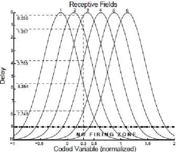
This encoding method can work perfectly well for a number of clusters less or equal to the number of dimensions, but its performance decreases when the number of clusters exceeds the number of input dimensions. The proposed solution for this problem [15] implemented here uses an encoding method based on population coding [16], which distributes an input variable over multiple input neurons. By this method, the input variables are encoded with graded and overlapping activation functions, modeled as local receptive fields. Fig. 3 shows the encoding of the value 0.3. In this case, assuming that the time unit is millisecond, the value 0.3 was encoded with six neurons by delaying the firing of neurons 1 (5.564ms), 2 (1.287ms), 3 (0.250ms),
4 (3.783ms) and 5 (7.741ms). Neuron 6 does not fire at all, since the delay is above 9ms and lays in the no firing zone. It is easy to see that values close to 0.3 will cause neurons 2 and 3 to fire earlier than the others, meaning that the better a neuron is stimulated, the nearer to ms it will fire. A value up to ms is assigned to the less stimulated neurons, and above this limit the neuron does not fire at all (see fig. 4).
1
Radial Basis Function network
2
Excitatory postsynaptic potential
From a biological point of view, we can think of the input neurons as if they were some sort of sensory system sending signals proportional to their excitation, defined by the Gaussian receptive fields. These neurons translate the sensory signals into delayed spikes and send them forward to the output neurons. In this work, the encoding was made with the analog variables normalized in the interval [0,1] and the receptive fields equally distributed, with the centers of the first and the last receptive fields laying outside the coding interval [0,1], as shown in fig. 3, there is another way to encode analog variables, very similar to the first, the only difference being that no center lays outside the coding interval and the width of the receptive fields is broader.
Both types of encoding can be simultaneously used, like in fig. 5, to enhance the range of detectable detail and provide multi-scale sensitivity [17]. The width and the Fig.2 Left: SNN with a bi-dimensional input formed by three
spiking neurons and two RBF-like output neurons. Right: two randomly generated clusters (crosses and circles), correctly separated by the SNN.
Figure. 3 Continuous input variable encoded by means of local receptive fields.
centers are defined by Eq. (1) and (2), for the first and second types, respectively. Unless otherwise mentioned, the value of used for the first type is 1.5 and 0.5 for the second.
2. Learning
Giving some background information and instances of the application of the models to simulate real neurons, these examples demonstrate the existence of a relationship between electrophysiology, bifurcations, and computational properties of neurons, showing also the foundations of the dynamical behavior of neural systems. The approach presented here implements the Hebbian reinforcement learning method [18] through a winner-takes-all algorithm [19], that its practical application in SNN is discussed in [20] and a more theoretical approach is presented in [21]. In a clustering task, the learning process consists mainly of adapting the time delays, so that each output neuron represents an RBF center. This purpose is achieved using a learning window or learning function [22], which is defined as a function of the time interval
between the firing times and . This function controls the learning process by updating the weights based on this time difference, as shown in Eq. (3), where
is the amount by which the weights are increased or decreased and is the learning rate.
( )
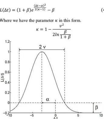
The learning function used here shown in fig. 6, is a Gaussian curve defined by the Eq. (4) [23]. It reinforces the synapse between neurons and , if �, and depresses the synapse if �.
Where we have the parameter in this form.
�
�
The learning window is defined by the following parameters:
-�: this parameter, called here neighborhood, determines the width of the learning window where it crosses the zero line and affects the range of , inside which the weights Fig. 5 Two ways to encode continuous input variable by means of
local receptive fields. The dotted lines are wide receptive fields of the second type, with �
Fig. 7 Gaussian learning function, with ��� �
are increased. Inside the neighborhood the weights are increased, otherwise they are decreased.
- : this parameter determines the amount by which the weights will be reduced and corresponds to the part of the curve laying outside the neighborhood and bellow the zero line.
- : because of the time constant of the EPSP, a neuron
firing exactly with does not contribute to the firing of , so the learning window must be shifted slightly to consider this time interval and to avoid reinforcing synapses that do not stimulate .
Since the objective of the learning process is to approximate the firing times of all the neurons related to the same cluster, it is quite clear that a neuron less stimulated (large and thus, low weight) must have also a lower time constant, so it can fire faster and compensate for the large . Similarly, a more stimulated neuron (small and thus, high weight) must have also a higher time constant, so it can fire slower and compensate for the small .
3. Conclusions
All the experimental results obtained in the development indicate that the simultaneous adaptation of weights and time constants (or axonal delays) must be submitted to a far more extensive theoretical analysis. Given the high complexity of the problem, it is not encompassed by the scope of the present work, and hence should be left to a further work. It was presented a practical applications of a neural network, built with more biologically inspired neuron, to perform what we could call real neuroscience task. In this application we demonstrated how analog values can be temporally encoded and how a network can learn using this temporal code. Even with these very short steps towards the realm of neuroscience, it is not difficult to realize how intricate things can get, if we try to descend deeper into the details of neural simulation. However, this apparent difficulty should rather be regarded as an opportunity to use spike-timing as an additional variable in the information processing by neural networks [24].
References
[1] Hernandez, Gerardina, Paul Munro, and Jonathan Rubin. "Mapping from the spike domain to the rate-based domain." Neural Information Processing, 2002. ICONIP'02. Proceedings of the 9th International Conference on. Vol. 4. IEEE, 2002.
[2] Aihara, Kazuyuki, and Isao Tokuda. "Possible neural coding with interevent intervals of synchronous firing." Physical
Review E 66.2 (2002): 026212.
[3] Yoshioka, Masahiko, and Masatoshi Shiino. "Pattern coding based on firing times in a network of spiking neurons." Neural Networks, 1999. IJCNN'99. International Joint Conference on. Vol. 1. IEEE, 1999.
[4] Araki, Osamu, and Kazuyuki Aihara. "Dual coding in a network of spiking neurons: aperiodic spikes and stable firing rates." Neural Networks, 1999. IJCNN'99. International Joint Conference on. Vol. 1. IEEE, 1999.
[5] Koch, Christof. Biophysics of computation: information processing in single neurons. Oxford university press, 1998. [6] Dayan, P. E. T. E. R., L. F. Abbott, and L. Abbott.
"Theoretical neuroscience: computational and mathematical modeling of neural systems." Philosophical Psychology (2001): 563-577.
[7]Maass, Wolfgang, and Christopher M. Bishop. Pulsed neural networks. MIT press, 2001.
[8] Gerstner, Wulfram, and Werner M. Kistler. Spiking neuron models: Single neurons, populations, plasticity. Cambridge university press, 2002.
[9] Wilson, Hugh Reid. Spikes, decisions, and actions: the dynamical foundations of neuroscience. Oxford University Press, 1999.
[10] Ruf, Berthold. Computing and learning with spiking neurons: theory and simulations. na, 1998.
[11] Snippe, Herman P. "Parameter extraction from population codes: A critical assessment." Neural Computation 8.3 (1996): 511-529.
[12] Gerstner, Wulfram. "Rapid signal transmission by populations of spiking neurons." IEE Conference Publication. Vol. 1. London; Institution of Electrical Engineers; 1999, 1999.
[13] Hopfield, John J. "Pattern recognition computation using
action potential timing for stimulus
representation." Nature 376.6535 (1995): 33-36.
[14] Maass, Wolfgang. "Networks of spiking neurons: the third generation of neural network models." Neural networks 10.9 (1997): 1659-1671.
[15]Avalos, Diego, and Fernando Ramirez. "An Introduction to Using Spiking Neural Networks for Traffic Sign Recognition." Sistemas Inteligentes: Reportes Finales Ene-May 2014} (2014): 41.
[16]de Kamps, Marc, and Frank van der Velde. "From artificial neural networks to spiking neuron populations and back again." Neural Networks 14.6 (2001): 941-953.
[17]Avalos, Diego, and Fernando Ramirez. "An Introduction to Using Spiking Neural Networks for Traffic Sign Recognition." Sistemas Inteligentes: Reportes Finales Ene-May 2014} (2014): 41.
[18]Morris, R. G. M. "DO Hebb: The Organization of Behavior, Wiley: New York; 1949." Brain research bulletin 50.5 (1999): 437.
[19] Haykin, Simon. "Adaptive filters." Signal Processing Magazine 6 (1999).
[20] Bohte, Sander M., Han La Poutré, and Joost N. Kok. "Unsupervised clustering with spiking neurons by sparse temporal coding and multilayer RBF networks."Neural Networks, IEEE Transactions on 13.2 (2002): 426-435. [21] Gerstner, Wulfram, and Werner M. Kistler. "Mathematical
formulations of Hebbian learning." Biological cybernetics 87.5-6 (2002): 404-415.
[23] Leibold, Christian, and J. Leo van Hemmen. "Temporal receptive fields, spikes, and Hebbian delay selection." Neural Networks 14.6 (2001): 805-813.
[24] Bohte, Sander M. "The evidence for neural information processing with precise spike-times: A survey." Natural Computing 3.2 (2004): 195-206.
First Author Master of science in neurophysics at Noshirvani Institute of Technology; analyzing visual information transmission in a network of neurons with feedback loop.