www.atmos-chem-phys.net/8/637/2008/
© Author(s) 2008. This work is distributed under the Creative Commons Attribution 3.0 License.
Chemistry
and Physics
Observations of iodine monoxide columns from satellite
A. Sch¨onhardt1, A. Richter1, F. Wittrock1, H. Kirk1, H. Oetjen1,*, H. K. Roscoe2, and J. P. Burrows1
1Institute of Environmental Physics, University of Bremen, Otto-Hahn-Allee 1, 28359 Bremen, Germany
2British Antarctic Survey, Natural Environment Research Council, High Cross, Madingley Road, Cambridge CB3 0ET, UK *now at: School of Chemistry, University of Leeds, Leeds, LS2 9JT, UK
Received: 23 July 2007 – Published in Atmos. Chem. Phys. Discuss.: 5 September 2007 Revised: 3 January 2008 – Accepted: 9 January 2008 – Published: 11 February 2008
Abstract. Iodine species in the troposphere are linked to ozone depletion and new particle formation. In this study, a full year of iodine monoxide (IO) columns retrieved from measurements of the SCIAMACHY satellite instrument is presented, coupled with a discussion of their uncertainties and the detection limits. The largest amounts of IO are found near springtime in the Antarctic. A seasonal variation of io-dine monoxide in Antarctica is revealed with high values in springtime, slightly less IO in the summer period and again larger amounts in autumn. In winter, no elevated IO levels are found in the areas accessible to satellite measurements. This seasonal cycle is in good agreement with recent ground-based measurements in Antarctica. In the Arctic region, no elevated IO levels were found in the period analysed. This implies that different conditions with respect to iodine re-lease exist in the two Polar Regions. To investigate possible release mechanisms, comparisons of IO columns with those of tropospheric BrO, and ice coverage are described and dis-cussed. Some parallels and interesting differences between IO and BrO temporal and spatial distributions are identified. Overall, the large spatial coverage of satellite retrieved IO data and the availability of a long-term dataset provide new insight about the abundances and distributions of iodine com-pounds in the troposphere.
1 Introduction
In recent times, measurements in the atmosphere and re-lated model studies have revealed the relevance of iodine species in the chemistry of the troposphere and the planetary boundary layer (Alicke et al., 1999; Vogt et al., 1999; Car-penter et al., 2003). Atmospheric models and measurement
Correspondence to:A. Sch¨onhardt (schoenhardt@iup.physik.uni-bremen.de)
methods to determine iodine compounds in the atmosphere were initially developed on account of radioactive iodine isotopes released from nuclear power installations and the need to understand their distribution and deposition (Cham-berlain and Chadwick, 1953; Cham(Cham-berlain, 1960; Chamber-lain et al., 1960). Models for the investigation of tropo-spheric iodine chemistry further evolved after the recogni-tion of significant release of methyl iodide into the tropo-sphere (Chameides and Davis, 1980; Chatfield and Crutzen, 1990). The importance of iodine in the atmosphere includes its role in tropospheric ozone depletion and its influence on new particle formation (O’Dowd et al., 1999, 2002a,b; Mc-Figgans et al., 2004). The potential significance of iodine for stratospheric chemistry has also been studied (Solomon et al., 1994). Information about the spatial and temporal distri-bution of iodine compounds is required to assess accurately their role in atmospheric chemistry. This is currently limited by the sparseness of available measurements. In this context, the detection of iodine monoxide (IO) from instrumentation aboard orbiting satellites has the potential to fill partially the lack of knowledge and thereby test and improve our under-standing of iodine chemistry. Recently, first studies on the retrieval of IO from the SCIAMACHY satellite instrument have been reported (Sch¨onhardt et al., 2007; Saiz-Lopez et al., 2007c). Both studies show enhanced column amounts of IO around Antarctica and demonstrate that the retrieval of IO from satellite is close to the limit of detection but possible.
During the last decade, IO has been observed in a vari-ety of atmospheric studies, primarily in the marine boundary layer (Alicke et al., 1999; Carpenter et al., 1999; Peters et al., 2005) in polar regions (Wittrock et al., 2000; Friess et al., 2001; Saiz-Lopez et al., 2007a), and also above the open ocean (Allan et al., 2000). In addition to IO, other relevant iodine compounds such as the iodine dioxide molecule OIO, molecular iodine I2, and organic iodocarbons have also been
iodocarbons including CH3I, CH2I2and CH2ICl emitted
di-rectly or indidi-rectly from algae, are thought to be the typical precursors of atomic iodine. At mid-latitudes, such as Mace Head in Ireland, a correlation of IO with solar irradiation and low tidal height exposing the emitting algae to air was identi-fied (Alicke et al., 1999; Carpenter et al., 1999; Peters et al., 2005).
In Polar Regions, the source of iodine is partly attributed to release of iodine containing organic compounds from ice algae (Reifenh¨auser and Heuman, 1992; Carpenter et al., 2007). However, inorganic mechanisms releasing iodine from sea salt or brine cannot be ruled out (Carpenter et al., 2005). In any case, effective and iodine selective re-lease from ocean water into the atmosphere via biogenic or inorganic pathways appears to exist at least locally. This is indicated by the enrichment of iodine compounds in the marine boundary layer, especially in marine aerosols, when compared to for example chlorine species (Reifenh¨auser and Heuman, 1992; Vogt et al., 1999). Typical tropospheric abun-dances of iodocarbons and subsequent iodine oxides lie in the range of 0 to several pptv (Carpenter et al., 1999; Allan et al., 2000; Peters et al., 2005) and are most probably confined to the lowest layers of the atmosphere (Friess et al., 2001). In some locations the amount of IO was below the detection limit while higher values of up to 10 pptv (Peters et al., 2005; Zingler and Platt, 2005) have been measured in several loca-tions at certain times. The currently highest amounts of up to 20 pptv (Saiz-Lopez et al., 2007a) and very recently 30 pptv (D. Heard, yet unpublished data) seem to be rather rare and transitory events.
In the stratosphere, IO could also contribute to ozone de-struction (Solomon et al., 1994) but mixing ratios are low compared to the high values observed in coastal hot spots. There has been some limited evidence for small amounts of IO in the polar spring in the northern hemispheric strato-sphere, but the upper limit for stratospheric IO mixing ratios is small (Wennberg et al., 1997; Pundt et al., 1998; Wittrock et al., 2000; B¨osch et al., 2003). In this study, the integrated IO column amounts retrieved from satellite nadir observa-tions are assigned to the tropospheric columns, assuming that the significant part of the IO column is situated in the bound-ary layer, in accordance with the observations reported thus far.
When emitted into the atmosphere, many iodine com-pounds rapidly photolyse releasing atomic iodine radicals, e.g. (CH2I2+hν→CH2I+I) or (I2+hν→I+I). Following the
reaction with ozone (O3), IO radicals then form initiating a
catalytic ozone destruction cycle in areas of iodine release (Solomon et al., 1994). Atomic iodine is regenerated by dif-ferent pathways, for example by the reaction with other halo-gen oxides (X=Br or Cl, Reactions R2, R3), or with HO2
(Reactions R4, R5) or NO2 (Reaction R8) and subsequent
photolysis.
I+O3→IO+O2 (R1)
XO+IO→I+X+O2 (R2)
X+O3→XO+O2 (R3)
Net:2O3→3O2
I+O3→IO+O2
IO+HO2→HOI+O2 (R4)
→OH+I+O2 (R5)
HOI+hν→OH+I (R6)
OH+O3→HO2+O2 (R7)
Net:2O3→3O2
IO+NO2+M→IONO2+M (R8)
IONO2+hν →I+NO3 (R9)
→IO+NO2 (R10)
The photolysis of IO regenerates I atoms (and ozone) and leads to some steady state amount of IO during daytime.
IO+hν→I+O (R11)
O+O2+M→O3+M (R12)
If no other chemistry were considered and as a result of the rapid photolysis of iodine compounds, IO would be expected to be the dominant gas phase iodine compound in the tropo-sphere. Similar to other halogen oxides like ClO and BrO (Molina and Rowland, 1974; Stolarski and Cicerone, 1974; Barrie et al., 1988), the presence of IO is linked to catalytic destruction of O3. However, the chain length of such
de-struction cycles depends on the termination reactions which produce higher oxides of iodine and lead to particle forma-tion.
In Polar Regions, springtime tropospheric ozone depletion events are frequently observed and have been linked to en-hanced bromine amounts (Barrie et al., 1988; Oltmans et al., 1989; Kreher et al., 1997, and references therein). The ob-servations of large clouds of BrO from satellites (Wagner and Platt, 1998; Richter et al., 1998; Burrows et al., 1999) at high latitudes was followed by the suggestion that areas with the potential to form frost flowers might be a major source region of these clouds (Kaleschke et al., 2004). The low temperatures of aerosol and possibly surface brine in such regions triggers the release of bromine (R. Sander et al., 2006), required to explain the bromine explosion (Platt and H¨onninger, 2003). However, model studies suggest that even small amounts of iodine can play an important role in the re-lease and recycling processes of Br atoms (Vogt et al., 1999). This further enhances the strength and impact of bromine ex-plosions seen in Polar Regions, making the catalytic ozone depletion even more effective.
G´omez Mart´ın et al., 2007, and references therein), the two relevant reaction pathways being
IO+IO→OIO+I (R13)
IO+IO+M→I2O2+M (R14)
Iodine oxides may be generated also by reaction pathways between IO and other halogen oxides (ClO or BrO) or possi-bly by minor channels of the reaction of IO with HO2, e.g.:
BrO+IO→OIO+Br (R15)
HO2+IO→OIO+OH (R16)
In any case, OIO or I2O2are liberated. Subsequently, higher
oxides (IxOy, such as I2O4and I2O5) are formed, which
re-act further with OIO, and can then cluster and precipitate (O’Dowd et al., 2002a; McFiggans et al., 2004; O’Dowd and Hoffmann, 2005). In addition, some of the higher iodine ox-ide clusters, being acid anhydrox-ides, are very hygroscopic. The mechanism, by which aerosols are formed, is not yet established. However, it has been shown that the formation of higher oxides results in the production of ultra-fine parti-cles. These may then grow to small aerosols and act as cloud condensation nuclei. These processes impact on the aerosol loading and potentially the amount of clouds and therefore also on the Earth’s radiation budget and climate forcing. In addition, it is now clear that iodine plays a significant role in both the homogeneous and heterogeneous chemistry of the troposphere, at least locally. The complete cycling of iodine in the atmosphere is still not well understood. Measurements of the global distribution of IO are needed to test our current knowledge and constrain atmospheric models describing io-dine behaviour.
The present study addresses the observation of IO from space. For this purpose, the absorption of IO is re-trieved from measurements of the back-scattered radiation up-welling from the atmosphere taken by the SCanning Imaging Absorption spectroMeter for Atmospheric CHartog-raphY (SCIAMACHY), a UV-vis-NIR spectrometer onboard the ENVISAT satellite (Burrows et al., 1995; Bovensmann et al., 1999). The sensitivity and detection limit of the satellite measurements with respect to IO in the atmospheric bound-ary layer are discussed, and a study of the spatial and sea-sonal variation of IO focussing on the southern hemispheric Polar Region is presented.
2 Instrument
The instrument SCIAMACHY is mounted on the ESA satel-lite ENVISAT, which was launched in March 2002. The in-strumental properties and mission objectives have been de-scribed in detail elsewhere (Burrows et al., 1995; Bovens-mann et al., 1999). The sun-synchronous, near-polar orbit of ENVISAT has a local equator crossing time of 10:00 a.m. in a descending node. SCIAMACHY makes measurements
4
0
5
0
6
0
3
0
2
0
1
0
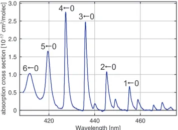
Fig. 1.Absorption cross section spectrum of iodine monoxide (Spi-etz et al., 2005) with an original FWHM of 0.07 nm, convoluted with the SCIAMACHY slit function. Eight excitation bands (six of them shown in the graph) from the ground state to the first excited
state with different vibrational levels (A23/2←X23/2) can be
identi-fied, resulting in a very strong differential structure.
of the transmitted, backscattered and reflected light from the Earth’s atmosphere or surface, observing in nadir and limb viewing geometries, as well as in solar and lunar occultation. The light is separated into eight spectral channels measuring simultaneously, with six contiguous channels between 240 and 1750 nm and two further short wave infrared channels. The alternate limb and nadir viewing coupled with a swath width of 960 km yields global coverage at the equator within six days.
In this study, the spectral absorption and scattering fea-tures in the blue part of the spectrum from the nadir mea-surements have been investigated. In order to optimise the signal-to-noise ratio, the size of the ground scene was in-creased to 60 km along and 120 km across track by averag-ing several individual measurements. A criterion restrictaverag-ing the solar zenith angle to less than 84◦ was used to exclude observations having an intrinsic low signal-to-noise ratio and reduced sensitivity to the lower troposphere. The time period analysed covers the years 2004–2006 but focuses on 2005.
3 Iodine monoxide absorption
of magnitude larger than that for NO2 in the same
spec-tral region which is routinely used for Differential Opti-cal Absorption Spectroscopy (DOAS) (Platt, 1994) measure-ments of NO2 in the troposphere and stratosphere. The
maximum absorption cross section of IO is approximately σmax(IO)=2.8×10⁻¹⁷cm2/molec at 298 K and will be used later in the discussion of the IO detection limit of SCIA-MACHY. The IO molecule is therefore an ideal trace gas for remote sensing by DOAS in spite of its lower abundance, compared to NO2.
4 IO retrieval algorithm
For the retrieval of IO from SCIAMACHY data, the well-established DOAS technique has been used in this study. In this method, a polynomial acts as a high-pass filter account-ing for all broadband features such as broadband absorption, scattering, and instrumental effects. All differential struc-tures in the spectrum remain for assignment to trace gases, which exhibit highly variable absorption structures, and the Ring effect, which results from the interaction of Raman scattering on air molecules with the solar Fraunhofer lines and molecular absorption features. The slant column densi-ties are determined by a non-linear least squares fitting pro-cedure for each measured spectrum. The conversion of the slant column density to a vertical column density requires the calculation of the appropriate air mass factor (AMF) de-termined by a radiative transfer model which accounts for the light path through the trace gas layer.
In the following, we consistently show and discuss the slant column values of IO and not the vertical columns, be-cause the use of a calculated AMF introduces another source of uncertainty, which in the case of IO is fairly large. In some cases, as further discussed in Sect. 5, the AMF can easily vary by a factor of 2 for different vertical profiles of IO. As the profile shape is not well known for IO, we will continue to use the slant column densities.
The DOAS retrieval was performed in the spectral fitting window from 416 to 430 nm, which contains two absorp-tion peaks of IO, the (ν′=4←ν′′=0) and (ν′=5←ν′′=0)
ab-sorption bands of theA23/2←X23/2transition, cp. Fig. 1. A broader spectral window extending to longer wavelengths in-cluding additionally the (ν′=3←ν′′=0) band was also tested.
This was less successful, because of a strong Ring structure at 431 nm. As the Ring effect results in the strongest differ-ential feature in this wavelength window for many regions on Earth, even small errors in the fitting of this effect can lead to a large and highly structured, stable residual, which can interfere with the trace gas absorption for weak atmospheric absorptions of IO. It was noted that this interference is largest for certain geometrical conditions over bright surfaces, such as ice or clouds. This results occasionally in large apparent IO columns but poor fitting residuals. To avoid this problem
around 431 nm, the fit was confined to the spectral bands at shorter wavelengths.
In the retrieval, a second order polynomial was applied, and absorption cross-sections from NO2 (223 K) and O3
(223 K) (Bogumil et al., 2003), a Ring spectrum (Vountas et al., 1998), as well as an undersampling correction (Chance, 1998) and an additive linear polynomial were included. In order to minimise the impact from the Ring effect and any residual instrument noise resulting from small differences in the viewing of the earth and the sun by the instrument, only earthshine spectra were used for fitting purposes. For the at-mospheric background spectrum in the DOAS fitting proce-dure, for each day of measurements, the earthshine spectrum from over the tropical Pacific (at 40◦S, 160◦W averaged
over the available spectra within ±10◦ in both directions)
was used. This is a region where the IO signal is expected to be small, which was confirmed by fitting this earthshine signal with the solar reference spectrum. The difference in the absorption optical depth between the background spec-trum and each individual satellite measurement is the basis for the DOAS analysis. The resulting slant column retrieved for each single satellite pixel is the difference in slant column between the amount at a specific position and this reference position.
In the present study, the retrieval of IO in the Antarctic region is of central interest. The underlying area is mostly ice/snow covered. Reliable separation of clouds from ice and snow is not routinely available yet, so no cloud screening was applied. Considering the influence of clouds, two aspects play a role and require consideration – the change in radiative transfer due to clouds and potential retrieval errors.
The location of the trace gas with respect to the cloud de-termines the effect of the change in radiative transfer. Most studies suggest that IO is mainly located close to the ground. This implies that the IO is situated below a cloud cover in this case. The sensitivity for detection will be reduced and some underestimation of the IO slant column may occur.
In addition, potential retrieval errors in cloudy scenes have to be ruled out. For ice free regions, cloud screening tests show, that no systematic retrieval error is introduced for IO measurements over clouds.
number of data points, but neither the absolute amount, nor the spatial pattern of IO is changed systematically.
In conclusion, the use of cloudy pixels in the data set does not lead to significantly larger retrieval errors, but may lead to a small underestimation of the IO slant columns.
5 Detection limit
In order to estimate the detection limits for IO columns re-trieved from SCIAMACHY measurements, several factors, determined by the instrument and those arising from assump-tions made in the retrieval algorithm, need to be accounted for. The minimal optical depth ODmindetectable by the
in-strument is determined primarily by the noise-to-signal ratio (N/S) of the measured spectrum, whereSis the number of electrons generated from incoming photons at the detector during a measurement, andN the value for the total noise arising in the measurement process. The ratioN/Sis deter-mined by the number of photons captured in one measure-ment and – in the selected spectral region – to a much lesser extent by the detector noise. It therefore depends on quanti-ties like wavelength, surface spectral reflectance and the solar zenith angle. For the photon signal falling on a detector pixel, N/Sis given to a good approximation by the shot noise in the electron flux, i.e.
N S =((N
2
i +Nd2)/S2)1/2
whereNiis the number of noise electrons generated from
in-coming photons, andNdis the number of noise electrons
de-termined by the dark signal for the individual detector pixel. For the wavelength region under consideration here, the root mean square (rms) of the optical depth is on the order of 10−4 for 90% surface spectral reflectance (No¨el et al.,
1998). For an ideal measurement, the slant column detec-tion limit (SClim) is given by the ratio of the residual rms
and σmax (the maximum differential absorption cross sec-tion value of the respective trace gas). This analysis assumes that a trace gas is detectable if the absorption optical depth SC×σmaxbecomes larger than the residual rms value. For IO slant columns and a surface spectral reflectance of 90%, the detection limit is given by SClim=7×10¹²molec/cm2for
a single measurement. This limit can be further reduced by averaging, in time or space, provided the source of er-rors is random and systematic erer-rors have been accounted for. For a surface spectral reflectance of 5% instead of 90%, the IO slant column detection limit for a single measure-ment corresponds to 2×10¹³molec/cm2. For 90% surface spectral reflectance and the spatially averaged ground scene of 60×120 km2, used in this study, the limit is reduced to 3×10¹²molec/cm2.
To convert the slant column detection limit to a mixing ra-tio detecra-tion limit, assumpra-tions on the appropriate air mass factor, and in particular on the altitude profile of IO are
nec-0 2 4 6 8 10
0 1 2 3 4 5 6
settings: Antarctica settings: Ireland
Block AMF
Altitude [km]
Fig. 2. Block air mass factors calculated with SCIATRAN Ver-sion 2.0 (Rozanov et al., 2005) for 425 nm, and two different
exam-ple locations, red: 90% albedo, 70◦solar zenith angle (typical for
Antarctica, October 2005), blue: 5% albedo, 55◦solar zenith angle
(typical for Ireland). For the boundary layer, the AMF and with this the sensitivity for IO detection is several times higher for Antarctic conditions.
essary. For this, radiative transfer calculations using the SCI-ATRAN V2.0 radiative transfer model (Rozanov et al., 2005) have been undertaken. For the wavelength of 425 nm, the AMF varies between 1.0 (for 5% surface spectral reflectance, 55◦ solar zenith angle, as at the Irish coast) and 4.2 (for
90% surface spectral reflectance, 70◦ solar zenith angle, as
in Antarctica), assuming an IO profile with constant mix-ing ratio in the lowest kilometre and a linear decrease to 0 at 2 km. For the high surface spectral reflectance case, the AMF changes only by a few percent even if IO is assumed to be well mixed only in the lowest 100 m, or up to 10 km. However, for the low surface spectral reflectance case, the AMF of the two scenarios varies by a factor of 2.
(a) (b)
Fig. 3. Typical fit results from 1 October 2005. The plots show the differential absorption (top), the remaining residual (bottom) and
inbetween the trace gas fits for NO2, the Ring effect and IO (including in each case the residual structure) compared to the respective scaled
reference cross section. (a)was taken at 70.7◦S, 53.7◦W with an IO amount of 2.1±0.5×10¹³molec/cm2, rms=1.7×10⁻⁴, and(b)at
the above values were calculated for a single measurement without any averaging. This analysis shows that the IO de-tection limit for a single SCIAMACHY ground scene lies close to and in some cases below the IO amounts observed by ground-based measurements. For these cases, positive de-tection of IO from satellite can be expected if the spatial ex-tent of the area of enhanced IO amounts is of the order of a satellite ground-pixel.
6 Results
DOAS retrievals of IO were undertaken on SCIAMACHY measurements using the procedure and assumptions de-scribed above. Typical fitting residuals exhibit rms values of around 1–2×10⁻⁴in terms of optical depth for a single
mea-surement. Two examples are shown in Fig. 3 for different amounts of detected IO slant columns. This figure displays the total differential absorption spectrum, the fits of NO2,
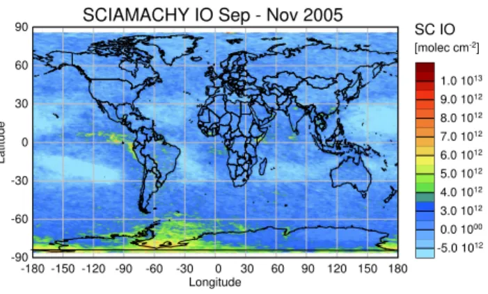
the Ring effect and IO from the measurement including in each case the residual noise in direct comparison with the scaled reference absorption cross section, and finally the fit residual. Assuming that a trace gas becomes detectable if its differential absorption structures are larger than the rms of the respective residual, an experimental detection limit of 5– 10×1012molec/cm2results for a single measurement. This limit is only slightly higher than the theoretically achievable limit discussed in the previous section. As a result of averag-ing the detection limit for the monthly mean drops to smaller values dependent on the square root of the number of mea-surements available for a specific location. This number is highly variable, ranging from no measurements at all close to the winter pole to up to five measurements a day, at high latitudes in summer. As a consequence, the detection limit in the monthly mean can improve by up to a factor of 5 or more. Global IO slant columns averaged over the months of September to November 2005 are shown colour coded on a global map in Fig. 4. The highest values in the monthly aver-age amount to about 8×10¹²molec/cm2and are detected in a widespread area close to Antarctica off the coast, especially in the Weddell Sea.
Surprisingly, enhanced IO amounts are also observed on the Antarctic continent. This is interesting, as these regions are situated at some distance from suspected sources of IO. Possible explanations for this unexpected finding are dis-cussed in Sect. 8.
Other regions with enhanced values are seen e.g. over the tropical Pacific west of Central America. It is interesting to note these small amounts of IO retrieved over up welling gions and biologically active oceans. However, in these re-gions, the signal-to-noise ratio of the retrieval is poorer and the results for IO columns are therefore more sensitive to fit settings. For example, a slight change in the fitting window can change these features strongly. Consequently, these val-ues have to be treated with caution and their significance will
-180 -150 -120 -90 -60 -30 0 30 60 90 120 150 180 Longitude
Latitude
-90 -60 -30 0 30 60 90
-5.0 1012 0.0 1000 3.0 1012 4.0 1012 5.0 1012 6.0 1012 7.0 1012 8.0 1012 9.0 1012 1.0 1013 SC IO
[molec cm-2]
SCIAMACHY IO Sep - Nov 2005
Fig. 4.Iodine oxide slant columns as retrieved from SCIAMACHY nadir measurements averaged over three months (September to November 2005). The highest values are found close to Antarctica, especially in the Weddell Sea.
require careful validation. In contrast, the maximum close to the Antarctic continent is stable with respect to the changes in the fit settings.
Closer inspection of the figure also reveals areas with neg-ative IO columns, mainly over the “ocean deserts” where the water is clear and the penetration of solar radiation signif-icant. This interference is attributed to incompletely com-pensated vibrational Raman scattering in water and/or weak water absorption in the water. This behaviour has been iden-tified also in the retrievals of other trace gas products in these regions. A more detailed modelling of the water-leaving ra-diance is expected to improve the fitting results.
There is no unambiguous indication from the results for enhanced IO columns in regions such as the Irish or Britannic coast, where ground-based measurements detected IO at high concentrations. This is probably the result of the larger de-tection limit at mid-latitudinal coastal sites and the spatially and temporally confined nature of the sources such as the fields of algae, which emit mainly during times of low tide along the coast. For the regions outside Antarctica, an up-per limit for monthly and spatially averaged IO is estimated to lie around 3×10¹²molec/cm2, while higher values within shorter time scales or locally might very well be present nev-ertheless. The results around Antarctica have been further analysed and the seasonal means of the IO differential slant column are plotted in Fig. 5 for the Southern Hemisphere.
Fig. 5.Seasonally averaged slant column amounts of IO above the Southern Hemisphere from Antarctic autumn to summer, explicitly for the periods of March–May, June–August, September–November 2005, and December 2005–February 2006. Maxima in IO columns occur over the Weddell Sea, the Ross Sea and along the coast especially in spring and in autumn with levels remaining positive at some places throughout the summer.
poles due to darkness, but even at the rim of the measurement region, in areas where IO exists in other times of the year, no systematically enhanced values are detected.
Very recently, a study of IO columns for four days of SCIAMACHY data has been published (Saiz-Lopez et al., 2007c). In agreement with the results presented here, high values are reported close to Antarctica in October 2005. However, some differences between the two data sets have been noticed, for example the maximal daily IO columns tend to be a few times lower in the present study. Addi-tionally, the spatial distributions of IO differ. While en-hanced values of IO spread mainly in the Weddell Sea and at the Antarctic continent in our analysis, in Saiz-Lopez et al. (2007c) the highest values were retrieved above sea ice regions between 60◦ and 70◦ Southern latitude, but in two
cases also well outside the ice covered regions over the ocean southwest of the South American continent, possibly related to cloud fields. Coupled with the different spectral windows used in the studies, this may in part explain the observed dif-ferences. Currently, the reasons for the differences have not yet been unambiguously identified but will be investigated when a longer time series of satellite data is available from the study of Saiz-Lopez et al. (2007c).
Overall, the DOAS fit yields reliable results in terms of the seasonal and spatial pattern, while the exact numbers of the IO slant column are subject to some remaining uncertainties. The quantitative analysis can only be further improved either by extending the fitting window to include three or more IO absorption peaks, after having solved the issues, discussed above with respect to residual features from strong Raman structures in that wavelength range or, by averaging of more spectra before starting the fit routine.
7 Comparison with ground-based measurements
(a)
-0.5 0 0.5 1.0 1.5
2004
J F M A M J J A S O N D
2005
J F M A M J J A S O N D
2006
J F M A M J J A S O N D J
SC IO Averaged IO
SC IO [ 10
13 molec/cm 2]
SCIAMACHY IO at Halley
(b)
Fig. 6.Seasonal variation of IO. The figure(a)shows SCIAMACHY IO slant columns within 500 km of Halley Station for the three years from 2004–2006; daily values in blue and a two week average in black. This seasonal cycle matches very well with ground based LP-DOAS
results, shown in(b). IO and BrO VMR values (single values and 10-day moving averages) are plotted versus time of year from February
2004–February 2005. Clearly, the maximum of IO around October, the minimum in Antarctic winter and the second smaller maximum in
autumn (March) are visible.(b)taken from Saiz-Lopez et al. (2007a). Reprinted with permission from AAAS.
from January 2004 until February 2005. Approximately at a distance of 12 km from the ocean, Halley Station is situ-ated on the Antarctic shelf ice. The LP-DOAS measurements yield the trace gas volume-mixing ratio (VMR) at 4–5 m el-evation above the ice surface averaged over the optical path length of 8 km. Assuming a vertical distribution of IO, which does not change over time, the conversion between a column amount and the VMR is given by a constant factor, and the general evolution of the two measurement series can be com-pared directly.
In Fig. 6a, a time series of IO slant column amounts from SCIAMACHY at Halley is shown, covering the three sub-sequent years from 2004 to 2006. This dataset takes into account all SCIAMACHY measurements within a square of 500 km side length enclosing Halley Station. Interest-ingly, the IO time series shows a repeating seasonal pat-tern. The months without data represent the polar winter pe-riods where scattered sunlight measurements are not possi-ble due to darkness. The maximum in IO values is found for all three years in springtime around October with av-erage values around 7×10¹²molec/cm2. The amounts
de-crease but remain positive throughout Antarctic summer and rise slightly towards February/March. The increase in AMF due to light path extension during the autumn and spring periods compared to the summer leads to slightly ampli-fied values of IO slant columns from satellite data for these times. However, the change in AMF from spring to summer is at most 15% and does not explain the observed seasonal variation in IO slant column amounts which ranges from 7×10¹²molec/cm2 down to 2×10¹²molec/cm2 in the av-eraged time series.
This observed pattern compares well with the ground-based LP-DOAS data from the CHABLIS campaign. For comparison with the satellite observations, this LP-DOAS dataset from the year 2004 is shown in Fig. 6b. The observed VMR of IO close to the ground is plotted versus the time of year. Also shown in this plot is the observed BrO amount at the same location. Both trace gases show the same evolution with their maxima and minima of concentrations at the same time of the year.
(a)
5.0 1013 5.5 1013 6.0 1013 6.5 1013 7.0 1013 7.5 1013 8.0 1013 >
< VC BrO [molec cm-2] SCIAMACHY BrO Oct 2005
(b) -5.0 10
12 0.0 1000 3.0 1012 4.0 1012 5.0 1012 6.0 1012 7.0 1012 8.0 1012 9.0 1012 1.0 1013 SC IO [molec cm-2] SCIAMACHY IO Oct 2005
(c)
Fig. 7. These maps show the comparisons of the distribution of(a)BrO,(b)IO, averaged for October 2005 and(c)the ice coverage on 15 October 2005 in the Southern Hemisphere. (c) Courtesy of L. Kaleschke and G. Spreen, University of Hamburg.
dark winter period, then a clear maximum of 7 pptv in the monthly mean in October (with single values up to 20 pptv), and lower but still positive values throughout the Antarctic summer. Consequently, highest values in both, satellite and ground-based measurements, are found for the time around October.
A direct quantitative comparison between the two mea-surement types requires an assumption on the vertical distri-bution of IO. For a constant IO VMR in the lowest 100 m dropping to zero above and a typical value of 4 for the AMF, the maximum in the averaged IO slant column in October, retrieved from satellite measurements corresponds to a VMR of 6–7 pptv, which is in good agreement with the LP-DOAS measurements within the experimental error.
For the northern high latitudes, a comparison of IO amounts has also been made with the ground-based MAX-DOAS (multi-axis MAX-DOAS) measurements from Ny- ˚Alesund on Spitsbergen (79◦N, 12◦E). Throughout the time when daylight is available, scattered sunlight spectra are recorded and provide local slant column densities of trace gases such as IO with some information on the height distribution. The instrumentation and retrieval method for the zenith-sky
the satellite measurement will fall close to or below the re-spective detection limit taking all data into consideration as in this study. Additionally, recent model studies suggest that the IO is only mixed to altitudes on the order of 100 m and decreases with height (Saiz-Lopez et al., 2007b). Such a pro-file leads to a higher surface concentration detection limit for the retrieval of IO from satellite. A campaign undertaken by the University of Bremen used the MAX-DOAS instru-mentation at the island of Sylt in Northern Germany during May 2005. IO was identified but the daytime values were low with columns being less than or equal to 3×10¹²molec/cm2
(H. Oetjen, yet unpublished results) also below the detection limit for observation from SCIAMACHY.
In agreement with these estimations, no systematically en-hanced amounts of IO have been identified over Spitsbergen or European coastal measurement sites in our analysis at any time of the year. In conclusion, the limited number of inde-pendent measurements of IO is in reasonable agreement with the magnitude and seasonal behaviour of the IO amounts ob-served in this study.
8 Discussion
The spatial and seasonal patterns of the IO columns observed from SCIAMACHY, yield information about the possible sources of IO, in particular when coupled with comparisons of the amounts and distributions of bromine oxide (BrO), and ice coverage. To investigate the relationship of IO with these other relevant parameters, Fig. 7 shows the southern hemi-spheric maps of the BrO vertical columns (a), the IO slant columns (b), and ice coverage (c) for October 2005. In addi-tion the possible connecaddi-tion of IO with organic precursors in the ocean is discussed.
8.1 IO and ice coverage
It is illuminating to compare the map of IO columns with that for the ice coverage in Antarctica (Fig. 7c). The ice coverage is determined from measurements by the AMSR-E (Advanced Microwave Scanning Radiometer for AMSR-EOS) in-strument onboard the AQUA satellite launched in May 2002, using the 89 GHz channels (Kaleschke et al., 2001; Spreen et al., 2008). The area with enhanced IO amounts is widely ex-tended throughout the Weddell Sea and reaches far over the ice covered area. This supports the proposal that iodine pre-cursors are correlated with or are dependent on conditions associated with sea ice at high latitudes. Potential release mechanisms include both a direct inorganic release of iodine from the mineral phase and the photolysis of organic iodocar-bon compounds, e.g. from the biosphere below and around the sea ice.
Both processes need to be particularly effective, as the io-dine in ioio-dine compounds originally derives from sea salt, where iodine concentration is fairly small. It should be noted
that the retrieval of IO from the SCIAMACHY measure-ments are intrinsically less sensitive to any IO present over open water which is not accounted for in the slant columns discussed here. This results from the noise being higher be-cause the surface spectral reflectance of the open ocean is lower than that of ice or snow.
8.2 Comparison between BrO and IO values
Enhanced concentrations of BrO are regularly observed over and close to sea ice in polar spring in connection with ozone depletion events and can be observed by satellite (e.g. Richter et al., 1998; Wagner and Platt, 1998). Compared to the dis-tribution of BrO in Antarctica, the observations of IO ex-hibit some similarities but also some interesting and signif-icant differences (Fig. 7a, b). In this context, the highest amounts of BrO are found in September, the values remain large throughout springtime and then decrease over the sum-mer with possibly slightly higher amounts of BrO in autumn. This differs from the situation for IO, which has two clear maxima, the first one in October and a second around March. Likewise, with respect to the spatial distribution of IO and BrO, similarities exist but the behaviours of IO and BrO are also significantly different. While the fact that both IO and BrO appear in the springtime in regions close to one another could be interpreted as indication for similar or even linked release mechanisms, the different spatial pattern found for these two compounds (see Fig. 7a and b) argues for different activation processes for reactive iodine and reactive bromine species. The region where highest BrO amounts are found is of a ring shape above all of the sea ice around the Antarctic continent having varying hot spots. In contrast, the largest IO columns are situated close to and partly overlapping the BrO regions, but they are concentrated further south around the Weddell Sea, along the Antarctic coast, and to some extent in the Ross Sea, including even the shelf ice regions, i.e. the Ross, the Filchner-Ronne and the Amery ice shelves, and also parts of the continent.
case for BrO, also short lived molecules can be transported over far distances if efficient recycling mechanisms exist.
One interesting hypothesis that might explain the ob-served IO amounts far from its sources combines biolog-ical emission of iodoorganic species, transport and trans-formation, deposition and aggregation of iodine compounds and snow photochemistry. Organic I is produced, e.g. by the maritime biosphere in the ocean, below and in the ice. The exact processes for this are not yet fully understood. When openings in the ice occur, organic iodine compo-nents are likely to be released, and eventually IO forms. At enhanced concentrations, IO produces higher oxides of I, which preferentially being hygroscopic attach to aerosols or themselves are aerosol condensation nuclei. The iodine in the aerosol or later cloud phase is then transported and deposited at the surface. In these regions, snow photo-chemistry (HNO3+hν→OH+NO2) results in local high IO
amounts via oxidation of HIO3 and other I compounds by
OH (OH+HIO3→H2O+IO3, IO3→IO+O2).
This hypothesis implies, that IO is recycled and reformed from the aerosol phase also at further distance from the sea ice. The suggested process and the corresponding chemistry serve as a possible explanation, and need to be subject of fur-ther research. Recycling of iodine from higher oxides and from sea-salt aerosol is needed for a longer effective lifetime of IO also in Saiz-Lopez et al. (2007b), which again is re-quired to explain some current observations of well-mixed IO in the boundary layer and the observed IO amounts at Halley Station (Sect. 7) at 12 km from the nearest coast.
The correlation between source regions of polar BrO clouds and regions of potential frost flower coverage (PFF) led to the proposal that bromine is released from brine in aerosols or on freshly formed sea ice and to subsequent dis-cussions (Kaleschke et al., 2004; Piot and von Glasow, 2007; R. Sander et al., 2006). The influence of PFF conditions on the release of iodine is not yet known or studied, but the spatial difference in BrO and IO fields observed indi-cates that PFF is not as strongly linked to IO as it might be to BrO. Maximum column amounts of BrO of up to 1×10¹⁴molec/cm2are about one order of magnitude higher
than that observed for IO. Taking the ratio of bromine to iodine ion concentrations in sea water of [Br]/[I]=15 000 (Wayne, 2000) and the removal processes for BrO and IO into account, any mechanism for iodine release compara-ble to that described for bromine requires a much more ef-ficient emission of iodine species or a highly iodine selec-tive process. As a consequence, additional pathways are re-quired to explain the release of reactive iodine into the at-mosphere over Antarctica. These processes coupled with the local transport need to be distributed widely, as the detected IO clouds appear to be spread over extended regions.
8.3 IO and organic precursors
By analogy with the well-known release of iodine species by macro-algae at mid-latitudinal coastal sites, iodine in the Antarctic is likely to originate at least partly from biologi-cal activity. Algae and other biologibiologi-cally active organisms in the cold water and ice have already been identified as a source of emissions of organic iodocarbons (Carpenter et al., 2007). The latter are reported to be present in the top layers of Antarctic water and below the ice, and they are released to the atmosphere by a variety of exchange processes. Depen-dent on the specific organism, various types of halocarbons are produced in different ratios (Laturnus et al., 2004). As a consequence, the amount of iodinated compounds in the ice and water, and those released to the atmosphere depends amongst other factors on the local biological activity.
The regions of maximum IO amounts in Antarctic spring and autumn are mostly covered with ice, but open water re-gions and breaking of, or transport through, leaking ice may lead to a flow of gaseous species from the ice, or the underly-ing water, into the atmosphere. In spite of the low light levels, species such as diatoms multiply in regions partly covered by ice, because it is favourable for them to be attached to the un-dersurface of the ice cover, and the cold ocean water is rich in nutrients. In addition, transfer from organic species within the ice sheets to the atmosphere above is probable. Diatoms grow fine underneath multi-year ice, which gets more porous when it ages, and nutrients are still supplied by the currents existing under sea ice. Considering the differences between BrO and IO observations discussed above, IO is located fur-ther south also in regions of older sea ice, where fur-therefore the biological pathway could be an explanation for the obtained results.
One useful indicator for biological activity in oceans, directly linked to the occurrence of photosynthesis is the chlorophyll-a pigment concentration. Available data of chlorophyll-a concentrations from satellite are currently lim-ited to open water regions larger than ca. 9 km. Open water leads and polynya in the ice, smaller than this value are not analysed. Even with a few percent ice within a ground pixel, the reflection from this area exceeds the weak signal reflected from the water that contains the information on chlorophyll concentration. Therefore, no data are available for the Wed-dell Sea and other ice covered regions, preventing any firm conclusions about the biogenic sources releasing iodine com-pounds in these regions.
a concurrence of the conditions of maximum release (and therefore high concentrations) of these precursors, and light levels sufficient for efficient photolysis. Consequently, dur-ing winter, IO amounts are expected to be low owdur-ing to the lack of actinic flux and low biological productivity.
From springtime onwards, when sunlight is available, the precursor substances are photolysed producing the required iodine radicals. Similarly, the growth of algae communities under the ice and the availability of leads and polynya in ice become significant. The decrease in IO amounts during sum-mer time may result from the changing biological activity, associated with the minimum in the sea ice cover. This in-ference is supported by the observation that organisms and biological activity are distributed over a deeper water col-umn in summer time, whereas they are more concentrated to-wards the surface facilitating exchange with the atmosphere in spring and autumn (Simpson et al., 2007). Additionally, a second bloom in sea-ice diatoms in Antarctica occurs in autumn, which also supports the explanation that biological pathways can at least partly cause the seasonal variation ob-served for IO.
8.5 IO in regions other than Antarctica
Interestingly, no notably enhanced IO amounts have been identified in the Arctic throughout the period analysed in contrast to the situation for BrO. The lower values in the Northern Hemisphere might be explained by the different bi-ological conditions at high latitudes in the Arctic as com-pared to the Antarctic. Iodocarbons have been found in the Arctic (Schall et al., 1994), but Arctic diatoms are a differ-ent species and the production of iodine compounds differs between the various species of algae. The differences in bio-logical activity impacts on the amounts of IO precursors, and the meteorology of the Arctic as compared to that around and above Antarctica is likely to lead to different patterns and amounts of IO for a predominantly biological source.
At mid and low latitudes, the poorer detection limit for the monthly mean IO composites as compared with high lat-itudes arises from the poorer frequency of measurements and from the lower surface spectral reflectance of oceans as com-pared to that of ice and snow in the IO spectral window. Con-sequently, observations of assured columns of IO above the respective detection limit in these regions from satellite mea-surements are not reported in this study. The observation of enhanced but noisy IO signals above biologically active regions including some up-welling regions such as off the coast of Peru is not further analysed here, but it should be noted nevertheless that this observation would be consistent with the source of IO being the production of iodine con-taining species by the oceanic biosphere and their direct or subsequent emission to the atmosphere.
8.6 Atmospheric significance of the retrieved IO column amounts
With the results from satellite measurements, the significance of iodine oxide in the atmosphere can be estimated. Un-less stated otherwise, rate coefficients used in this section are taken from S. P. Sander et al. (2006).
The reaction of I atoms with O3 initiates a chain
reac-tion removing ozone, which in addireac-tion to bromine chemistry contributes to the understanding of the low daytime amounts of tropospheric O3observed in the remote marine boundary
layer (von Glasow et al., 2002; Dickerson et al., 1999, and references therein).
For the following calculation, the upper limit of 3×10¹²molec/cm2 in marine areas for the IO vertical col-umn (for AMF=1) and a marine boundary layer of typi-cally 0.5 to 2.5 km height are considered. Assuming that the IO column is confined to a well-mixed marine bound-ary layer, and assuming to a first order approximation that I, IO and O3 achieve a stationary state determined by
Re-actions (R1), (R11) and (R12), the ratio [I]/[IO] would be given by J(R11)/k(R1)[O3]. With O3 mixing ratios between
1 to 40 ppbv, and J(R11) between 0.03 and 0.24 s−1(G´omez
Mart´ın et al., 2006; Harwood et al., 1997), the [I]/[IO] ra-tio lies in the range from 0.025 to 8. In model studies by Vogt et al. (1999), the ratio [Br]/[BrO] lies around 0.035– 0.07 in a base run, while [I]/[IO] from the above estimate yields a ratio of 0.35 if the same atmospheric conditions as in that model run are applied. Considering the approximated O3loss rates of k(R1)[I][O3] for the iodine cycle and in
anal-ogy k(R1)[Br][O3] for the bromine cycle, this means that even
if BrO amounts are higher than IO amounts by one order of magnitude, the O3loss rates lie in the same range. In
compar-ison, model studies by von Glasow et al. (2002) infer that the presence of small amounts of iodine increases tropospheric ozone loss by up to 40%.
The potential for particle formation in the marine bound-ary layer by iodine chemistry needs to be addressed. Higher iodine oxides, which can form adducts with water, and iodine oxide clusters act as condensation nuclei for aerosol forma-tion. As the rate of higher oxide production depends on the square of the IO concentration, this is a highly non-linear process. The upper limit for the rate of particle formation R(I-aerosol) is given by the rate of higher oxide formation, i.e. R(I-aerosol)≈(k(R13)+k(R14))[IO]2.
For comparison, the formation of particles from sulphur species is estimated. For this, H2SO4is a crucial substance,
and its average rate of formation is determined by the rate of the three body reaction of OH with SO2(OH + SO2+ M→
HOSO2+ M), as subsequent reactions forming H2SO4 are
rapid.
We assume the reaction rate k(OH+SO2+M)at its high
pres-sure limit and daytime marine boundary layer conditions for SO2 (100 pptv) and OH (1×10⁶molec/cm3). The rate
(followed by formation of aerosol) is determined by R(S-aerosol)≈k(OH+SO2+M)[OH][SO2] and can be compared to
the rate of formation of the higher iodine oxides (R13, R14) for the given assumptions.
With kIO+IO=8×10⁻¹¹cm3/molec/s and
(k(R13)+k(R14))/kIO+IO close to 1 (Bloss et al., 2001),
the ratio of these rates, R(I-aerosol)/R(S-aerosol) varies between (<2 to 72)×102. Possibly, iodine could be a
significant source of atmospheric aerosol in the remote marine boundary layer in addition to that from the oxidation of sulphur. In this context, it is already known that iodine chemistry is a significant local source of new particles (O’Dowd and Hoffmann, 2005; McFiggans et al., 2004). Detailed models, taking into account the non-linearity of the iodine and sulphur chemistry and including accurate estimates of the release of DMS and iodine atom precursors and also of the final clustering probabilities, are required to assess accurately the relative importance of iodine chemistry as a global source of particles.
9 Summary and conclusions
Using nadir measurements from the SCIAMACHY satellite instrument, global maps of the IO column density were re-trieved for the years 2004 to 2006, with a focus on 2005, by means of the DOAS retrieval method. The theoretical de-tection limit of a few 1012molec/cm2 lies close to the ex-pected IO amounts observed thus far by ground-based mea-surements. For a given VMR in the ground layer, the ap-plicability of satellite measurements for IO columns strongly depends on surface spectral reflectance of the ground scene and the height to which IO is mixed, i.e. the vertical profile of IO, in the atmosphere. However, in regions of enhanced IO amounts and high surface reflectivity, the unambiguous detection of IO with SCIAMACHY is possible.
Close to Antarctica, large areas, exhibiting IO amounts considerably above the detection limit for the retrieval of IO columns from SCIAMACHY, have been identified dur-ing the period from sprdur-ing to autumn. The highest monthly average values of IO slant columns are found for October and March (springtime and autumn) close to the Antarctic continent, especially in the Weddell Sea, and amount up to 8×10¹²molec/cm2, while values on single days can be sig-nificantly higher.
A seasonal variation of IO columns in the Antarctic region is revealed, in which the IO columns show generally low val-ues in winter, as far as these regions are accessible to satel-lite measurements, a maximum during springtime, decreas-ing values durdecreas-ing summer and a second peak in Antarctic au-tumn. This seasonal pattern is confirmed by a long-term time series of three years of data around Halley Station, Antarc-tica, where this same behaviour is repeated every year. Com-paring this time series of satellite observations to ground-based measurements at Halley (Saiz-Lopez et al., 2007a),
good agreement is achieved within the respective error lim-its for this seasonal evolution of IO amounts. No enhanced amounts of IO could be seen for the Arctic region throughout the period analysed, indicating some systematic differences in the availability of precursor substances between the north-ern and southnorth-ern hemispheric polar regions.
Ice cover maps show that positive detection of IO reaches over large ice covered areas in Antarctica, revealing some correlation of enhanced IO amounts with ice coverage and supporting the connection of ice to the release of reactive io-dine. This implies that direct abiotic and/or biogenic sources of iodine are probably associated with the ice sheets.
A comparison between IO and BrO maps reveals differ-ences in the spatial and temporal distribution of these two halogen oxides. Some similarities such as the occurrence of IO and BrO maxima in the Antarctic springtime support the concept that chemistries of these halogen oxides are to some extent coupled and may have some common sources, but the differences in the patterns provide evidence that significantly different sources of bromine and iodine are required. These findings for the IO distributions are interpreted as indicating the existence of a biological source of iodocarbons and pos-sibly I2, which act as precursors of reactive iodine.
Sufficient solar actinic irradiation for the photolysis of the iodine containing species in the boundary layer represents another necessary condition for the production of IO. This condition explains part of the observed seasonality of IO at high latitudes.
Knowledge of the seasonal variations of the not yet fully identified release processes are needed to complete and en-hance our understanding in the future. For a more conclusive interpretation of IO more detailed information on the biologi-cal situation, emission properties of the sea ice layers and the chemical cycles involved are needed. Similarly, modelling of the complex iodine and sulphur chemistry of the remote marine boundary is necessary to assess accurately the mag-nitude of the catalytic loss of O3and the number density of
particles originating from the chemistry of iodine. However, the magnitude and distribution of the IO columns observed in this study indicates that both of these processes could be of potential local and even global significance for tropospheric chemistry.
Acknowledgements. This study has been supported by the State and University of Bremen, the German Aerospace (DLR), and
the European Union. It has benefited from the EU ACCENT
project. ESA and the DLR kindly provided the level 1 data from SCIAMACHY used in this study. We would like to thank the British Antarctic Survey, the NERC and especially A. Saiz-Lopez and J. M. C. Plane for the kind provision of ground-based data from the CHABLIS campaign as well as L. Kaleschke for helpful
discussions and provision of ice maps. Finally, we also thank
M. Vountas and W. Lotz for their support and for providing the PMD cloud and surface product prior to its publication.
References
Alicke, B., Hebestreit, K., Stutz, J., and Platt, U.: Iodine oxide in the marine boundary layer, Nature, 397–398, 572, 1999. Allan, B. J., McFiggans, G., Plane, J. M. C., and Coe, H.:
Observa-tions of iodine monoxide in the remote marine boundary layer, J. Geophys. Res., 105, 14 363–14 369, 2000.
Barnes, W. L., Pagano, T. S., and Salomonson, V. V.: Prelaunch characteristics of the Moderate Resolution Imaging Spectrora-diometer (MODIS) on EOS-AM1, IEEE Trans. Geosci. Rem. Sens., 36(4), 1088–1100, 1998.
Barrie, L. A., Bottenheim, J. W., Schnell, R. C., Crutzen P. J., and Rasmussen, R. A.: Ozone destruction and photochemical reac-tions at polar sunrise in the lower Arctic atmosphere, Nature, 334, 138–141, 1988.
Bloss, W. J., Rowley, D. M., Cox, R. A., and Jones, R. L.: Kinetics and Products of the IO Self-Reaction, J. Phys. Chem. A, 105, 7840–7854, 2001.
Bogumil, K., Orphal, J., Homann, T., Voigt, S., Spietz, P., Fleis-chmann, O. C., Vogel, A., Hartmann, M., Bovensmann, H., Frerik, J., and Burrows, J. P.: Measurements of Molecular Ab-sorption Spectra with the SCIAMACHY Pre-Flight Model: In-strument Characterization and Reference Data for Atmospheric Remote-Sensing in the 230–2380 nm Region, J. Photochem. Photobiol. A., 157, 167–184, 2003.
B¨osch, H., Camy-Peyret, C., Chipperfield, M. P., Fitzenberger, R., Harder, H., Platt, U., and Pfeilsticker, K.: Upper limits of strato-spheric IO and OIO inferred from center-to-limb-darkening-corrected balloon-borne solar occultation visible spectra: Impli-cations for total gaseous iodine and stratospheric ozone, J. Geo-phys. Res., 108(D15), 4455, doi:10.1029/2002JD003078, 2003. Bovensmann, H., Burrows, J. P., Buchwitz, M., Frerick, J., No¨el,
S., Rozanov, V. V., Chance, K. V., and Goede, A. P. H.: SCIA-MACHY: Mission Objectives and Measurement Modes, J. At-mos. Sci., 56, 127–150, 1999.
Burrows, J. P., H¨olzle, E., Goede, A. P. H., Visser, H., and Fricke, W.: SCIAMACHY – Scanning Imaging Absorption Spectrome-ter for Atmospheric Chartography, Acta Astronautica, 35, 445– 451, 1995.
Burrows, J. P., Weber, M., Buchwitz, M., Rozanov, V. V., Ladst¨atter-Weißenmayer, A., Richter, A., DeBeek, R., Hoogen, R., Bramstedt, K., and Eichmann, K. U.: The Global Ozone Monitoring Experiment (GOME): Mission Concept and First Scientific Results, J. Atmos. Sci., 56, 151–175, 1999.
Carder, K. L., Chen, F. R., Cannizzaro, J. P., Campbell, J. W., and Mitchell, B. G.: Performance of the MODIS semi-analytical ocean color algorithm for chlorophyll-a, Adv. Space Res., 33, 1152–1159, 2004.
Carpenter, L. J., Sturges, W. T., Penkett, S. A., Liss, P. S., Alicke, B., Hebestreit, K., and Platt, U.: Short-lived alkyl iodides and bromides at Mace Head, Ireland: Links to biogenic sources and halogen oxide production, J. Geophys. Res., 104, 1679–1689, 1999.
Carpenter, L. J.: Iodine in the Marine Boundary Layer, Chem. Rev., 103, 4953–4962, 2003.
Carpenter, L. J., Hopkins, J. R., Jones, C. E., Lewis, A. C., Parthipan, R., Wevill, D. J., Poissant, L., Pilote, M., and Con-stant, P.: Abiotic Source of Reactive Organic Halogens in the Sub-Arctic Atmosphere?, Environ. Sci. Technol., 39, 8812– 8816, 2005.
Carpenter, L. J., Wevill, D. J., Palmer, C. J., and Michels, J.: Depth profiles of volatile iodine and bromine-containing halocarbons in coastal Antarctic waters, Mar. Chem., 103, 227–236, 2007. Chamberlain, A. C. and Chadwick, R. C.: Deposition of airborne
radioactive vapour, Nucleonics, 11, 22–25, 1953.
Chamberlain, A. C.: Deposition of iodine-131 in Northern England in October 1957, Q. J. Roy. Meteor. Soc., 85, 350–361, 1960a. Chamberlain, A. C., Eggleton, A. E. J., Megaw, W. J., and Morris,
J. B.: Behaviour of Iodine Vapour in air, Disc. Faraday Soc., 30, 162–169, 1960.
Chameides, W. L. and Davis, D. D.: Iodine: its possible role in tropospheric chemistry, J. Geophys. Res., 85, 7383–7398, 1980. Chance, K.: Analysis of BrO Measurements from the Global Ozone Monitoring Experiment, Geophys. Res. Lett., 25, 3335–3338, 1998.
Chatfield, R. B. and Crutzen, P. J.: Are there interactions of iodine and sulfur species in marine air photochemistry?, J. Geophys. Res., 95, 22 319–22 341, 1990.
Cox, R. A. and Coker, G. B.: Absorption Cross Section and Kinetics
of IO in the Photolysis of CH3I in the Presence of Ozone, J. Phys.
Chem., 87, 4478–4484, 1983.
Cox, R. A., Bloss, W. J., Jones, R. L., and Rowley, D. M.: OIO and the Atmospheric Cycle of Iodine, Geophys. Res. Lett., 26, 1857–1860, 1999.
Dickerson, R. R., Rhoads, K. P., Carsey, T. P., Oltmans, S. J., Crutzen, P. J., and Burrows, J. P.: Ozone in the remote marine boundary layer: a possible role for halogens, J. Geophys. Res., 104(D17), 21 385, doi:10.1029/1999JD900023, 1999.
Friess, U., Wagner, T., Pundt, I., Pfeilsticker, K., and Platt, U.: Spectroscopic Measurements of Tropospheric Iodine Oxide at Neumeyer Station, Antarctica, Geophys. Res. Lett., 28(10), 1941, doi:10.1029/2003JD004133, 2001.
G´omez Mart´ın, J. C.: Spectroscopic, Kinetic and Mechanistic
Stud-ies of Atmospherically Relevant I2/O3 Photochemistry, PhD
Thesis, University Bremen, 2006.
G´omez Mart´ın, J. C., Spietz, P., and Burrows, J. P.: Kinetic and
Mechanistic Studies of the I2/O3Photochemistry, J. Phys. Chem.
A., 111(2), 306, doi:10.1021/jp061186c, 2007.
Harwood, M. H., Burkholder, J. B., Hunter, M., Fox, R. W., and Ravishankara, A. R.: Absorption Cross Sections and Self-Reaction Kinetics of the IO Radical, J. Phys. Chem. A, 101, 853– 863, 1997.
H¨onninger, G., Leser, H., Sebasti´an, O., and Platt, U.: Ground-based measurements of halogen oxides at the Hudson Bay by active longpath DOAS and passive MAX-DOAS, Geophys. Res. Lett., 31, L04111, doi:10.1029/2003GL018982, 2004.
Kaleschke, L., L¨upkes, C., Vihma, T., Haarpaintner, J., Bochert, A., Hartmann, J., and Heygster, G.: SSM/I Sea Ice Remote Sensing for Mesoscale Ocean-Atmosphere Interaction Analysis, Can. J. Rem. Sens., 27, 526–537, 2001.
Kaleschke, L., Richter, A., Burrows, J. P., Afe, O., Heygster, G., Notholt, J., Rankin, A. M., Roscoe, H. K., Hollwedel, J., Wagner, T., and Jacobi, H.-W.: Frost flowers on sea ice as a source of sea salt and their influence on tropospheric halogen chemistry, Geophys. Res. Lett., 31, L16114, doi:10.1029/2004GL020655, 2004.
Chem. Phys. 5, 2729–2738, 2005.
Kreher, K., Johnston, P. V., Wood, S. W., Nardi, B., and Platt, U.: Ground-based measurements of tropospheric and stratospheric BrO at Arrival Heights, Antarctica, Geophys. Res. Lett., 24, 3021–3024, 1997.
Laturnus, F., Svensson, T., Wiencke, C., and ¨Oberg, G.:
Ultravio-let Radiation Affects Emission of Ozone-DepUltravio-leting Substances by Marine Macroalgae: Results from a Laboratory Incubation Study, Environ. Sci. Technol. 2004, 38, 6605–6609.
Molina, M. J. and Rowland, F. S.: Stratospheric sink for chloroflu-oromethanes: chlorine atom catalysed destruction of ozone, Na-ture, 249, 810–814, 1974.
McFiggans, G., Coe, H., Burgess, R., Allan, J., Cubison, M., Al-farra, M. R., Saunders, R., Saiz-Lopez, A., Plane, J. M. C., Wevill, D. J., Carpenter, L. J., Rickard, A. R., and Monks, P. S.: Direct evidence for coastal iodine particles from Laminaria macroalgae – linkage to emissions of molecular iodine, Atmos. Chem. Phys., 4, 701–713, 2004,
http://www.atmos-chem-phys.net/4/701/2004/.
No¨el, S., Bovensmann, H., Burrows, J. P., Frerick, J., Chance, K. V., Goede, A. H. P., and Muller, C.: The SCIAMACHY instrument on ENVISAT-1, Sensors, Systems, and Next-Generation Satel-lites II, Proc. SPIE, 3498, pp. 94–104, 1998.
O’Dowd, C. D., McFiggans, G., Creasey, D. J., Pirjola, L., Hoell, C., Smith, M. H., Allan, B. J., Plane, J. M. C., Heard, D. E., Lee, J. D., Pilling, M. J., and Kulmala, M.: On the photochemical pro-duction of new particles in the coastal boundary layer, Geophys. Res. Lett., 26, 1707–1710, 1999.
O’Dowd, C. D., Jimenez, J. L., Bahreini, R., Flagan, R. C., Seinfeld, J. H., Hameri, K., Pirjola, L., Kulmala, M., Jennings, S. G., and Hoffmann, T.: Marine aerosol formation from biogenic iodine emissions, Nature, 417, 632–636, 2002a.
O’Dowd, C. D., H¨ameri, K., M¨akel¨a, J. M., Pirjola, L., Kulmala, M., Jennings, S. G., Berresheim, H., Hansson, H.-C., de Leeuw, G., Kunz, G. J., Allen, A. G., Hewitt, C. N., Jackson, A., Viisa-nen, Y., and Hoffmann, T.: A dedicated study of New Particle Formation and Fate in the Coastal Environment (PARFORCE): Overview of objectives and achievements, J. Geophys. Res., 107(D19), 8108, doi:10.1029/2001JD000555, 8108, 2002b. O’Dowd, C. D. and Hoffmann, T.: Coastal New Particle Formation:
A Review of the Current State-Of-The-Art, Environ. Chem., 2, 245, doi:10.1071/EN05077, 2005.
Oltmans, S. J., Schnell, R. C. Sheridan, P. J., Peterson, R. E., Li, S.-M., Winchester, J. W., Tans, P. P., Sturges, W. T., Kahl, J. D., and Barrie, L. A.: Seasonal surface ozone and filterable bromine relationship in the high Arctic, Atmos. Environ., 23(11), 2431– 2441, 1989.
Peters, C., Pechtl, S., Stutz, J., Hebestreit, K., H¨onninger, G., Heumann, K. G., Schwarz, A., Winterlik, J., and Platt, U.: Re-active and organic halogen species in three different European coastal environments, Atmos. Chem. Phys., 5, 3357–3375, 2005, http://www.atmos-chem-phys.net/5/3357/2005/.
Piot, M. and von Glasow, R.: The potential importance of frost flowers, recycling on snow, and open leads for Ozone Depletion Events, Atmos. Chem. Phys. Discuss., 7, 4521–4595, 2007, http://www.atmos-chem-phys-discuss.net/7/4521/2007/. Platt, U.: Differential optical absorption spectroscopy (DOAS),
Chem. Anal. Series, 127, 27–83, 1994.
Platt, U. and H¨onninger, G.: The role of halogen species in the
troposphere, Chemosphere, 52, 325–338, 2003.
Pundt, I., Pommereau, J.-P., Phillips, C., and Lateltin, E.: Upper limits of iodine oxide in the lower stratosphere, J. Atmos. Chem., 30, 173–185, 1998.
Reifenh¨auser, W. and Heuman, K. G.: Determination of methyl io-dide in the Antarctic atmosphere and the south polar sea, Atmos. Environ., 26A(16), 2905–2912, 1992.
Richter, A., Wittrock, F., Eisinger, M., and Burrows, J. P.: GOME Observations of Tropospheric BrO in Northern Hemispheric Spring and Summer 1997, Geophys. Res. Lett., 25, 2683–2686, 1998.
Rozanov, A., Rozanov, V.-V., Buchwitz, M., Kokhanovsky, A., and Burrows, J. P.: SCIATRAN 2.0. A new radiative transfer model for geophysical applications in the 175–2400 nm spectral region, Adv. Space Res., 36, 1015–1019, doi:10.1016/j.asr.2005.03.012, 2005.
Saiz-Lopez, A., Shillito, J. A., Coe, H., and Plane, J. M. C.:
Mea-surements and modelling of I2, IO, OIO, BrO and NO3in the
mid-latitude marine boundary layer, Atmos. Chem. Phys., 6, 1513–1528, 2006a.
Saiz-Lopez, A., Mahajan, A. S., Salmon, R. A., Bauguitte, S. J.-B., Jones, A. E., Roscoe, H. K., and Plane, J. M. C.: Bound-ary layer halogens in coastal Antarctica, Science, 317, 348, doi:10.1126/science.1141408, 2007a.
Saiz-Lopez, A., Plane, J. M. C., Mahajan, A. S., Anderson, P. S., Bauguitte, S. J.-B., Jones, A. E., Roscoe, H. K., Salmon, R. A., Bloss, W. J., Lee, J. D., and Heard, D. E.: On the vertical distri-bution of boundary layer halogens over coastal Antarctica:
im-plications for O3, HOx, NOxand the Hg lifetime, Atmos. Chem.
Phys. Discuss., 7, 9385–9417, 2007b.
Saiz-Lopez, A., Chance, K., Liu, X., Kurosu, T. P., and Sander, S. P.: First observations of iodine oxide from space, Geophys. Res. Lett., 34, L12812, doi:10.1029/2007GL030111, 2007c. Schall, C., Laturnus, F., and Heumann, K. G.: Biogenic volatile
organoiodine and organobromine compounds released from po-lar macroalgae, Chemosphere, 28, 1315–1324, 1994.
Sander, R., Burrows, J. P., and Kaleschke, L.: Carbonate precipita-tion in brine – a potential trigger for tropospheric ozone depleprecipita-tion events, Atmos. Chem. Phys., 6, 4653–4658, 2006,
http://www.atmos-chem-phys.net/6/4653/2006/.
Sander, S. P., Finlayson-Pitts, B. J., Friedl, R. R., Golden, D. M., Huie, R. E., Keller-Rudek, H., Kolb, C. E., Kurylo, M. J., Molina, M. J., Moortgat, G. K., Orkin, V. L., Ravishankara, A. R., and Wine, P. H.: Chemical Kinetics and Photochemical Data for Use in Atmospheric Studies, Evaluation Number 15, JPL Publication 06-2, Jet Propulsion Laboratory, Pasadena, 2006.
Sch¨onhardt, A., Richter, A., Wittrock, F., Kirk, H., and Burrows, J. P.: First observations of atmospheric iodine oxide columns from satellite, Geophys. Res. Abstr., 9, 00592, 2007.
Simpson, W. R., von Glasow, R., Riedel, K., Anderson, P., Ariya, P., Bottenheim, J., Burrows, J. P., Carpenter, L., Frieß, U., Goodsite, M. E., Heard, D., Hutterli, M., Jacobi, H.-W., Kaleschke, L., Neff, B., Plane, J. M. C., Platt, U., Richter, A., Roscoe, H. K., Sander, R., Shepson, P., Sodeau, J., Steffen, A., Wagner, T., and Wolff, E.: Halogens and their role in polar boundary-layer ozone depletion, Atmos. Chem. Phys., 7, 4375–4418, 2007,
http://www.atmos-chem-phys.net/7/4375/2007/.
1994.
Spietz, P., Gomez Martin, J. C., and Burrows, J. P.:
Spec-troscopic studies of the I2/O3 photochemistry, Part 2:
Im-proved Spectra of Iodine Oxides and Analysis of the IO Ab-sorption Spectrum, J. Photochem. Photobiol. A, 176, 50–67, doi:10.1016/j.jphotochem.2005.08.023, 2005.
Spreen, G., Kaleschke, L., and Heygster, G.: Sea Ice Remote Sens-ing usSens-ing AMSR-E 89 GHz Channels, J. Geophys. Res., 113, C02S03, doi:10.1029/2005JC003384, 2008.
Stolarski, R. S. and Cicerone, R. J.: Stratospheric Chlorine: a Pos-sible Sink for Ozone, Can. J. Chem., 52, 1610–1615, 1974. Vogt, R., Sander, R., von Glasow, R., and Crutzen, P. J.: Iodine
Chemistry and its role in Halogen Activation and Ozone Loss In the Marine Boundary Layer: A Model Study., J. Atmos. Chem., 32, 375–395, 1999.
von Glasow, R., Sander, R., Bott, A., and Crutzen, P. J.: Modeling halogen chemistry in the marine boundary layer. 1. Cloud-free MBL, J. Geophys. Res., 107, 4341, doi:10.1029/2001JD000942, 2002.
Vountas, M., Rozanov, V. V., and Burrows, J. P.: Ring effect: Impact of rotational Raman scattering on radiative transfer in Earth’s at-mosphere, J. Quant. Spectrosc. Radiat. Transfer, 60(6), 943–961, 1998.
Wagner, T. and Platt, U.: Satellite mapping of enhanced BrO con-centration in the troposphere, Nature, 395, 486–490, 1998. Wayne, R. P.: Chemistry of Atmospheres, 3rd edition, Oxford
Uni-versity Press, 2000.
Wennberg, P. O., Brault, J. W., Hanisco, T. F., Salawitch, R. J., and Mount, G. H.: The atmospheric column abundance of IO: im-plications for stratospheric ozone, J. Geophys. Res., 102, 8887– 8898, 1997.
Wittrock, F., M¨uller, R., Richter, A., Bovensmann, H., and Burrows, J. P.: Measurements of Iodine monoxide (IO) above Spitsbergen, Geophys. Res. Lett., 27, 1471–1474, 2000.
Wittrock, F., Oetjen, H., Richter, A., Fietkau, S., Medeke, T., Rozanov, A., and Burrows, J. P.: MAX-DOAS measurements
of atmospheric trace gases in Ny- ˚Alesund – Radiative transfer
studies and their application, Atmos. Chem. Phys., 4, 955–966, 2004,
http://www.atmos-chem-phys.net/4/955/2004/.