www.atmos-meas-tech.net/6/2607/2013/ doi:10.5194/amt-6-2607-2013
© Author(s) 2013. CC Attribution 3.0 License.
Atmospheric
Measurement
Techniques
A new stratospheric and tropospheric NO
2
retrieval algorithm for
nadir-viewing satellite instruments: applications to OMI
E. J. Bucsela1, N. A. Krotkov2, E. A. Celarier2,3, L. N. Lamsal2,3, W. H. Swartz2,4, P. K. Bhartia2, K. F. Boersma5,6, J. P. Veefkind5, J. F. Gleason2, and K. E. Pickering2
1SRI International, Menlo Park, CA 94025, USA
2Laboratory for Atmospheres, NASA Goddard Space Flight Center, Greenbelt, MD 20771, USA 3Universities Space Research Association, Columbia, MD 21044, USA
4Applied Physics Laboratory, The Johns Hopkins University, Laurel, MD 20723, USA 5Royal Netherlands Meteorological Institute, De Bilt, the Netherlands
6Eindhoven University of Technology, Eindhoven, the Netherlands
Correspondence to:E. J. Bucsela ([email protected])
Received: 20 November 2012 – Published in Atmos. Meas. Tech. Discuss.: 7 February 2013 Revised: 12 July 2013 – Accepted: 1 August 2013 – Published: 15 October 2013
Abstract.We describe a new algorithm for the retrieval of nitrogen dioxide (NO2) vertical columns from nadir-viewing satellite instruments. This algorithm (SP2) is the basis for the Version 2.1 OMI This algorithm (SP2) is the basis for the Version 2.1 Ozone Monitoring Instrument (OMI) NO2 Stan-dard Product and features a novel method for separating the stratospheric and tropospheric columns. NO2Standard Prod-uct and features a novel method for separating the strato-spheric and tropostrato-spheric columns. The approach estimates the stratospheric NO2directly from satellite data without us-ing stratospheric chemical transport models or assumus-ing any global zonal wave pattern. Tropospheric NO2 columns are retrieved using air mass factors derived from high-resolution radiative transfer calculations and a monthly climatology of NO2 profile shapes. We also present details of how uncer-tainties in the retrieved columns are estimated. The sensitiv-ity of the retrieval to assumptions made in the stratosphere– troposphere separation is discussed and shown to be small, in an absolute sense, for most regions. We compare daily and monthly mean global OMI NO2retrievals using the SP2 al-gorithm with those of the original Version 1 Standard Prod-uct (SP1) and the Dutch DOMINO prodProd-uct. The SP2 re-trievals yield significantly smaller summertime tropospheric columns than SP1, particularly in polluted regions, and are more consistent with validation studies. SP2 retrievals are also relatively free of modeling artifacts and negative tropo-spheric NO2values. In a reanalysis of an INTEX-B
valida-tion study, we show that SP2 largely eliminates an ∼20 % discrepancy that existed between OMI and independent in situ springtime NO2SP1 measurements.
1 Introduction
Nitrogen oxides are important atmospheric trace gases that have significant impacts on human health. The two princi-pal nitrogen oxides, nitric oxide (NO) and nitrogen diox-ide (NO2) (collectively NOx), play key roles in atmospheric aerosol formation and tropospheric ozone chemistry (e.g., Finlayson-Pitts and Pitts, 1999; Seinfeld and Pandis, 1998). Major sources of tropospheric NOxinclude combustion, soil emissions, and lightning. In the lower troposphere, NO2is a toxic gas and a precursor to tropospheric ozone through the reaction of NOx with volatile organic compounds (VOCs). In the stratosphere, NOxcontributes to both production and loss cycles of ozone and may indicate long-term changes in tropospheric emissions of nitrous oxide (N2O), an important greenhouse gas. Stratospheric NOx is produced mainly by the reaction of N2O with O(1D).
Early spectroscopic ground-based measurements of NO2 were described by Brewer et al. (1973), Noxon (1975), and Solomon and Garcia (1984). Global retrievals from satel-lite spectra became available beginning in the middle 1990s, including measurements by the Global Ozone Monitoring Experiment (GOME) instrument (1995–2003) (Burrows et al., 1999), continued by the Scanning Imaging Spectrom-eter for Atmospheric Cartography (SCIAMACHY) instru-ment (2002–2012) (Bovensmann et al., 1999), and currently by the Ozone Monitoring Instrument (OMI) (Levelt et al., 2006; Bucsela et al., 2006; Boersma et al., 2007, 2011) and GOME-2 (Callies et al., 2000; Valks and Loyola, 2008; Valks et al., 2011) instrument.
Satellite and in situ measurements of tropospheric nitro-gen oxides are used with chemical transport models (CTMs) to quantify sources and transport of NO2 pollution from power plants, automobiles, ships, and aircraft (e.g., Martin et al., 2003, 2006; Zhang et al., 2007; Beirle et al., 2004, 2011; Jaeglé et al., 2005; Frost et al., 2006; Boersma et al., 2008; Lin et al., 2010; Russell et al., 2010). Instruments on satellite platforms are particularly valuable, since they can obtain NO2measurements over large geographical regions. Top-down NO2 measurements are helpful in constraining emissions for global- and regional-scale atmospheric mod-els (Martin et al., 2003; Choi et al., 2008; Lamsal et al., 2010). Multiyear, consistent time-series measurements al-low the study of interannual variability and long-term trends (Richter et al., 2005), which have been used to assess the effectiveness of emission control regulations and the effects of economic trends on industrial activity (Frost et al., 2006; Kim et al., 2006; Castellanos and Boersma, 2012). NOx pro-duced by lightning (LNOx) contributes an additional 10– 15 % to total NOxproduction in the troposphere (Schumann and Huntrieser, 2007), and LNOxmeasurements are helpful in estimating the global NOxbudget (Tie et al., 2002; Martin et al., 2007).
In unpolluted areas, the stratospheric NO2 can exceed 90 % of the total NO2 column (Martin et al., 2002a). The partitioning of NOxand NOyin the stratosphere is sensitive to photochemical conditions; thus, NO2 has a strong diur-nal dependence that varies as a function of latitude and sea-son (Dirksen et al., 2011). Although NO2in the stratosphere is more zonally symmetric than in the troposphere, there is still spatial structure that is important for understanding the morphology of stratospheric NO2itself, while complicating the retrieval of tropospheric NO2from satellite-derived slant columns. The accuracy of the inferred tropospheric contri-bution critically depends on the characterization and separa-tion of stratospheric NO2. The procedure used to determine the two components of the NO2vertical column will be re-ferred to as the stratosphere–troposphere separation (STS) al-gorithm.
Determining the relative amounts of stratospheric and tro-pospheric NO2 from a given absorption spectrum is inher-ently difficult. Although the shape of the NO2 absorption
cross section varies with altitude (due to temperature), cross sections at different temperatures are not orthogonal. There-fore, the stratospheric and tropospheric NO2amounts cannot be independently determined from the spectral fit. Instead, most STS algorithms rely on spatial information from mul-tiple slant columns measured over a wide geographic area. All such algorithms are prone to errors associated with the a priori information assumed about the stratospheric verti-cal column. The reference-sector (RS) method, discussed by Richter and Burrows (2002) and Boersma et al. (2004), as-sumes zonal invariance. The stratospheric vertical column at any latitude is set equal to the measured total column at the same latitude in the central Pacific Ocean. Because the central Pacific contains small background amounts of tropo-spheric NO2, the RS method can slightly overestimate the stratospheric fraction of the column. Martin et al. (2002a) corrected this by using model estimates of Pacific tropo-spheric NO2. More importantly, the real stratotropo-spheric NO2 varies with longitude, leading to potential inaccuracies in both the stratospheric and derived tropospheric vertical col-umn. Other methods, such as the image processing technique (IPT) of Leue et al. (2001) and Velders et al. (2001), and the wave-2 stratospheric model of Bucsela et al. (2006), allow for some longitudinal variation in stratospheric NO2. How-ever, like the RS method, the IPT and wave-2 algorithms re-quired relatively simplistic assumptions about which regions to use in constructing the global NO2stratospheric field. The wave-2 model, in particular, can introduce stratospheric ar-tifacts, especially at high latitudes (Dirksen et al., 2011). Some approaches have tried to capture more realistic struc-ture in the stratospheric NO2 field by using CTMs to esti-mate the spatial variation in stratospheric NO2. In the Dutch OMI NO2(DOMINO) product (Boersma et al., 2011; Dirk-sen et al., 2011), OMI NO2measurements are assimilated in a CTM model. CTM-based algorithms require daily model runs and relatively complex assimilation schemes. As will be shown, CTM-based algorithms can also introduce occa-sional modeling artifacts. If independent stratospheric mea-surements are available, a more observation-based approach can be used. Beirle et al. (2010) and Hilboll et al. (2013) have described methods for combining nadir measurements from OMI or SCIAMACHY with limb measurements of strato-spheric NO2from SCIAMACHY. Because the limb measure-ments are sparsely sampled, these approaches require signifi-cant spatial interpolation to obtain a continuous stratospheric field.
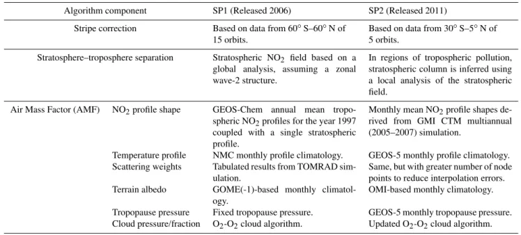
Table 1.Comparison of SP1 and SP2.
Algorithm component SP1 (Released 2006) SP2 (Released 2011)
Stripe correction Based on data from 60◦S–60◦N of 15 orbits.
Based on data from 30◦S–5◦N of 5 orbits.
Stratosphere–troposphere separation Stratospheric NO2 field based on a
global analysis, assuming a zonal wave-2 structure.
In regions of tropospheric pollution, stratospheric column is inferred using a local analysis of the stratospheric field.
Air Mass Factor (AMF) NO2profile shape GEOS-Chem annual mean
tropo-spheric NO2profiles for the year 1997
coupled with a single stratospheric profile.
Monthly mean NO2profile shapes
de-rived from GMI CTM multiannual (2005–2007) simulation.
Temperature profile NMC monthly profile climatology. GEOS-5 monthly profile climatology. Scattering weights Tabulated results from TOMRAD
sim-ulation.
Same, but with greater number of node points to reduce interpolation errors. Terrain albedo GOME(-1)-based monthly
climatol-ogy.
OMI-based monthly climatology.
Tropopause pressure Fixed tropopause pressure. GEOS-5 monthly tropopause pressure. Cloud pressure/fraction O2-O2cloud algorithm. Updated O2-O2cloud algorithm.
the use of model information in retrievals, but includes a number of features not present in SP1. The SP2 stratospheric slant column is estimated from the total slant column using an a priori monthly tropospheric NO2model climatology, but only where tropospheric contamination of the observed NO2 column is below a threshold. The threshold is set by an upper limit on the amount that tropospheric NO2absorption may contaminate the observed stratospheric vertical column. The SP2 algorithm also features improved air mass factors based on new radiative transfer calculations and terrain reflectivi-ties and uses monthly, rather than annual, mean NO2profile shapes. Cloud properties are obtained from the OMI OM-CLDO2 data product, which has recently been updated to include better wavelength calibration, look-up tables using sun-normalized radiances, and cloud pressures clipped at the surface pressures (Maarten Sneep, private communication).
The purpose of this paper is twofold: (1) to introduce the new STS algorithm and (2) to discuss the additional, more incremental changes that distinguish SP2 from SP1. We de-scribe the algorithm in Sect. 2 and list the differences be-tween the old and new retrieval approaches. We present er-ror analysis in Sect. 3 and discuss additional considerations and comparisons with other datasets in Sect. 4. Although a thorough treatment of validations comparing the new algo-rithm with independent datasets is beyond the scope of this paper, a validation example is included in Sect. 4. Numer-ous additional validation studies will be presented separately by Lamsal et al. (2013). Section 5 contains a summary and conclusions.
2 Algorithm description
The architecture of the algorithm is summarized in the flow diagram in Fig. 1. Spectral data are fitted to obtain raw NO2 slant columns, S′ (Sect. 2.1), and are corrected for instru-mental artifacts (also referred to as striping; see Sect. 2.3) to yield the de-striped slant columns, S. The data are an-alyzed to separate stratospheric and tropospheric NO2 par-tial vertical columns,VstratandVtrop, and to obtain total col-umn amounts,Vtotal(Sect. 2.4). The stratospheric and tropo-spheric air mass factors,AstratandAtrop(Sect. 2.2), used in the calculations are based on a priori information from ra-diative transfer (RT) and CTM models. The RT calculations used to process the OMI data in this study were carried out using TOMRAD (Davé, 1965). Some details in the SP2 al-gorithm are similar to the approach used in SP1, but there are many important changes. The similarities and differences are summarized in Table 1, and details of the SP2 algorithm are presented in Sects. 2.1–2.4.
2.1 OMI spectral fitting
The NO2 slant columns used in this study were extracted from OMI spectra. The OMI instrument is a UV-VIS hyper-spectral, push-broom, nadir-viewing satellite spectrometer (Levelt et al., 2006) on the NASA EOS Aura satellite (Schoe-berl et al., 2006), launched in July 2004. Aura has an Equator crossing time of 13:30 LST and an orbital period of 99 min so that OMI views the entire sunlit portion of the Earth in
Fig. 1.Flow diagram of retrieval algorithm for stratospheric and tro-pospheric NO2columns.S,V,A, andSWrepresent slant-column
density, vertical-column density, air mass factor, and scattering weight (m), respectively. The section outlined in blue is OMI-specific. TOMRAD is a forward vector radiative transfer model (Davé, 1965).
to northern terminator on the sunlit side of the earth. Swaths in adjacent orbits are nearly contiguous at the Equator and overlap elsewhere. LST differences from the west to east sides of a swath range from approximately 1.5 h at the Equa-tor to several hours at mid- to high latitudes.
The NO2slant columns are estimated by spectral fitting of OMI earthshine radiances. The fitting algorithm uses the Dif-ferential Optical Absorption Spectroscopy (DOAS) method (Platt and Stutz, 2006), applied in the spectral range of 405 nm to 465 nm (Boersma et al., 2002; Bucsela et al., 2006). The earthshine radiances are normalized by a ref-erence OMI-measured solar irradiance spectrum [R(λ)=
I (λ)/F (λ)]. The use of a static measured solar reference spectrum reduced much of the calibration-induced striping that was discovered soon after OMI operations began (Dob-ber et al., 2008). (The removal of residual striping is de-scribed in Sect. 2.3). The normalized spectra,R(λ), are fit-ted to laboratory-measured trace gas absorption spectra at a fixed stratospheric temperature (T0=220 K), a reference ring spectrum (Chance and Spurr, 1997), and a polynomial function that models the spectrally slowly varying scatter-ing by clouds and aerosols and reflection by the Earth’s sur-face. In the current version, the only trace gas absorption spectra considered are those of NO2(Vandaele et al., 1998), O3(Bass and Johnsten, 1975), and H2O (Harder and Brault, 1997). The temperature dependence of the NO2 cross sec-tion is accounted for later in the algorithm. The trace gas absorption spectra used were produced by convolving high-resolution, laboratory-measured absorption spectra with the measured OMI slit function, measured pre-launch by Dirk-sen et al. (2006). The result of the spectral fit is the raw slant-column density for each OMI pixel.
The calibrations of the 60 cross-track FOVs have relative biases that are observed to be persistent on time scales of several orbits to several days. As a result, the retrieved NO2 slant columns show a pattern of stripes running along each orbital track. This instrumental artifact can be corrected to
some extent using the “de-striping” procedure described in Sect. 2.3. A more severe effect is the “row anomaly” (RA), which was first noticed in the data in June 2007 and is likely caused by an obstruction in part of OMI’s aperture. The ex-tent of the RA has increased since 2007 and currently af-fects approximately half of the FOVs. Current RA informa-tion is available at http://www.knmi.nl/omi/research/product/ rowanomaly-background.php. Users of OMI data are dis-couraged from using FOVs flagged as RA-affected.
2.2 Air mass factors
In DOAS retrievals, the air mass factor, A, is the ratio of a slant column, S, to the vertical column, V, we want to retrieve. We write this relationship generically asA=S/V. The air mass factor is assumed to be wavelength-independent across the slant-column fitting window. In a given partial at-mospheric region (stratosphere or troposphere), the air mass factor is computed as the ratio of the sum over layers of the slant sub-columnsSi to the sum of vertical sub-columnsVi:
A= S
V =
6iSi 6i Vi
, (1)
whereiis the layer index. The summation combines all lay-ers in the appropriate partial atmospheric column. Tempera-ture is assumed to be constant within a layer. Slant and verti-cal sub-columns can be represented as integrals over all pres-surespwithin layeri:
Si=κ
Z
i
dp·ζ (p)·m(p)·α(p) (2)
and
Vi=κ
Z
i
dp·ζ (p). (3)
Here, m(p) is the atmospheric scattering weight (also re-ferred to as the “box” or “layer” air mass factor), α(p) is a temperature-correction factor for the NO2absorption cross section,ζ(p) is the a priori NO2mixing ratio, andκis a con-stant equal to the reciprocal of the weight of an air molecule. The formulation in Eqs. (2) and (3) implicitly decouples at-mospheric scattering and NO2 absorption, as described by Palmer et al. (2001), so that them(p) are independent of NO2 amount. The temperature factorα(p) is needed to correct for the fixed-temperature NO2cross section (T0= 220 K) used in the slant-column fitting and can be written as a function of the local temperatureT(p) as
α(p)=1−0.003· [T (p)−T0]. (4)
in line with temperature correction coefficients proposed in Boersma et al. (2002, 2004).
For partly cloudy scenes, we use an independent-pixel approximation for the air mass factor (e.g., Martin et al., 2002a) and express scattering weights as the weighted sum of cloudy and clear components,m(p)cloudy andm(p)clear, respectively:
m(p)=w·m(p)cloudy+(1−w)·m(p)clear. (5) Here the weighting factor,w, denotes cloud/aerosol radiance fraction (CRF), the fraction of the measured radiation that comes from clouds and aerosols. In the SP1 and SP2 al-gorithms, aerosols are not distinguished from clouds, since weakly absorbing aerosols can have similar effects on the air mass factor in some circumstances (Boersma et al., 2011). The effect of stratospheric aerosols is also not explicitly con-sidered in the algorithm. The value ofw is generally larger than the O2-O2 geometrical cloud fraction at 470 nm since the clouds are assumed to be optically thick with an ef-fective Lambertian albedo of 0.8 (Stammes et al., 2008). The cloudy and clear scattering weights for a given obser-vation depend on parameters including viewing geometry, surface (terrain or cloud) pressure, and surface reflectivity. Scattering weights are computed and stored a priori in six-dimensional look-up tables (LUT) generated from a radiative transfer model. For clear-sky scattering weights, the six LUT parameters are solar zenith angle (SZA), viewing zenith an-gle (VZA), relative azimuth anan-gle (RAA), terrain reflectivity (Rt), terrain pressure (Pt), and atmospheric pressure level, (p). For cloudy scattering weights, we treat clouds as opaque Lambertian surfaces and replace the terrain reflectivity and terrain pressure with cloud reflectivity (Rc=0.8) and cloud optical centroid pressure (Pc), respectively. The latter is esti-mated with the OMI O2-O2cloud algorithm (Acarreta et al., 2004; Sneep et al., 2008; M. Sneep et al., private communi-cation, 2012).
The SP2 scattering weights are computed from parameter sets that have been improved relative to SP1. In particular, the terrain reflectivities, which were derived from GOME (Koelemeijer et al., 2003) in SP1, are now based on OMI measurements (Kleipool et al., 2008). Terrain pressures are obtained as described by Boersma at al. (2011) from a 3 km digital elevation model provided with the Aura data. The re-flectivities and other parameters are no longer assumed to vary linearly between tabulated values, as was the case in SP1, and are now interpolated using Lagrange polynomials. The resolution in the six-dimensional parameter space has also been increased. In the new algorithm, the number of nodal points in SZA, VZA, RAA,Rt,Pt, andpare 9, 6, 5, 8, 6, and 35, respectively. These improvements reduce inter-polation errors noted in SP1 (Dirksen et al., 2011) by up to 15 %.
The a priori NO2 mixing ratio profiles for the air mass factor calculations in SP2 are obtained 4 from the Global
Modeling Initiative (GMI) CTM (Duncan et al., 2007; Stra-han et al., 2007). The model simulates the stratosphere and troposphere and includes emissions, aerosol microphysics, chemistry, deposition, radiation, advection, and other im-portant chemical and physical processes, such as lightning NOx production (Duncan et al., 2007). The GMI chemi-cal mechanism combines the stratospheric mechanism de-scribed by Douglass et al. (2004) with a detailed tropospheric O3-NOx-hydrocarbon chemistry originating from the Har-vard GEOS-Chem model (Bey et al., 2001) and is driven by GEOS-5 meteorological fields at the resolution of 2◦ lat-itude ×2.5◦ longitude (Rienecker et al., 2008). The verti-cal extent of the model is from the surface to 0.01 hPa, with 72 levels and a vertical resolution ranging from∼150 m in the boundary layer to ∼1 km in the free troposphere and lower stratosphere. The tropopause pressure is defined in the GEOS-5 reanalysis driving the CTM using a combination of Ertel’s potential vorticity (EPV) and potential tempera-ture. The tropopause pressure is taken as the higher of the EPV = 3.6×10⁻⁶K kg−1m2s−1 and 385 K theta surfaces. For the NO2SP2 algorithm, the use of alternative tropopause definitions (e.g., a chemical tropopause) was found to have little effect on the retrieval, since the differences in pressure were generally small and occured in regions where NO2 con-centrations are low.
Model outputs were sampled at the LST of OMI over-pass, and monthly mean profiles were derived using four years (2004–2007) of simulation. In contrast, SP1 used an-nual mean tropospheric profiles for 1997 from a GEOS-Chem simulation (Bey et al., 2001; Martin et al., 2002b), with only a single profile used for the stratosphere (Bucsela et al., 2006). Unlike the stratospheric air mass factor, which depends mainly on the viewing geometry, the air mass factor in the troposphere is particularly sensitive to the NO2profile shape. Model profile shapes vary by geographic region and exhibit daily variability as well, as validated by in situ mea-surements (e.g., Boersma et al., 2008; Bucsela et al., 2008). Our sensitivity studies indicated that monthly mean profiles captured the seasonal variation sufficiently well so that daily profiles were not included in the SP2 algorithm; however, use of 30-day running mean NO2profile shapes is being consid-ered for a future version of the algorithm.
2.3 De-striped slant columns
–
Fig. 2.Maps of 21 March 2005 OMI NO2data showing STS algorithm steps.(a)Slant columns.(b)Vinit.(c)Vinitminus a priori troposphere.
(d)Same as(c), but masked for pollution (white areas correspond to a masking threshold of 0.3×1015cm−2).(e)Gridded,Vo
stratwith masked
areas interpolated.(f)Hot spots removed.(g)Stratosphere after final smooth, re-interpolated onto OMI pixel coordinates.(h)Tropospheric field.
from the mean slant column ‹S′›i and stratospheric air mass
factor ‹Astrat›i for that cross-track position and the
aver-age slant column ‹‹S′›i› and average stratospheric air mass
factor ‹‹Astrat›i› over the entire swath from 30◦S to 5◦N.
The computation of the entire swath averages excludes all scan positions that have extreme values of ‹S′›
i/‹Astrat›i
(> 1017cm−2) and those known, a priori, to be affected by the row anomaly. The initial bias estimate is
δi=‹S′›i− [‹Astrat›i·‹‹S′›i›/‹‹Astrat›i›]. (6)
The final value of the cross-track bias is recomputed from Eq. (6) by applying an additional screening criterion in the calculation of ‹‹S′›i› and ‹‹Astrat›i›. The cross-track scan
positions whoseδi values lie outside a ±2σ interval are
ex-cluded to ensure that very high or low values of the bias in any of the cross-track scan positions (including those
af-fected by the RA) do not affect the average. The resulting cross-track bias for a given OMI orbit is a set of 60 correc-tion constants. At each pixel in the orbit, the corresponding bias is subtracted from the measured slant columnS′to give a corrected (“de-striped”) slant columnS.
2.4 Stratosphere–troposphere separation (STS)
The STS scheme described in this study takes advantage of the fact that, over most of the Earth, the NO2absorption con-tributing to the slant-column measurements is almost entirely stratospheric. Therefore, a simple and reasonable initial esti-mate of the stratospheric vertical column is the ratio of the de-striped measured slant column to the (nearly geometric) stratospheric air mass factor:
In areas with relatively little tropospheric NO2, we obtain the value of the stratospheric vertical column by subtracting a fixed model estimate of the (small) tropospheric column fromVinitand applying spatial smoothing to the resultant ge-ographic field. Where there is substantial tropospheric NO2 pollution, the stratosphere is estimated by spatial interpola-tion from the surrounding clean regions. The tropospheric vertical column is then computed as the difference betweenS
and the stratospheric slant column, divided by a tropospheric air mass factor.
Figure 2 illustrates the steps of the STS algorithm for one day of data, beginning with the spectrally fitted slant columns (Fig. 2a) and initial vertical columnsVinit(Fig. 2b). The fol-lowing seven steps summarize subsequent computations.
1. Subtract an a priori troposphere fromVinitto get initial stratospheric vertical column.
2. Mask the field wherever tropospheric contamination exceeds a threshold.
3. Bin this initial stratospheric vertical-column estimate onto a geographic grid.
4. Interpolate the binned vertical columns over masked areas.
5. Identify and eliminate “hot spots” in the stratospheric field.
6. Smooth and interpolate to pixel-center coordinates to give the finalVstratat each FOV.
7. Subtract the stratospheric contribution to get the tropo-spheric vertical column.
For steps 1 and 2, we first compute an a priori tropospheric slant column,Strop, at each satellite pixel:
Strop=Vtrop_a_priori·Atrop, (8) where Vtrop_a_priori is a geographically gridded (2◦ lati-tude×2.5◦longitude), monthly mean model of NO
2 clima-tology of tropospheric vertical columns, andAtropis the tro-pospheric air mass factor. The NO2climatology used in com-putingVtrop_a_prioriis the same as that used in the calculation ofAtrop.
The initial estimate of the stratospheric fieldVstrato (Fig. 2c) is computed as
Vstrato =(S−Strop)/Astrat. (9) The algorithm then masksVstrato for all pixels in which the tro-pospheric contamination of the NO2column is large. Masked pixels, shown as white areas in Fig. 2d, are eliminated from the stratospheric field calculation. The masking threshold is chosen to exclude pixels whereVinitwould exceed the actual
stratospheric vertical column by more than a valueε. We re-quire
(Strop/Astrat) < ε. (10) In the current algorithm, we chose an absolute threshold of ε= 0.3×1015cm−2 to limit the stratospheric vertical-column uncertainty introduced by the a priori troposphere to a value of 0.2×1015cm−2 or less. This uncertainty is con-sistent with previous estimates of uncertainty in the strato-spheric NO2 column (see Sect. 3.2) and is comparable to pixel noise associated with the slant-column uncertainty (see Sect. 3). Using this masking scheme allows polluted pixels to remain unmasked where the lower troposphere is obscured by clouds. These unmasked pixels provide a more robust stratospheric retrieval in polluted areas than would be pos-sible if all polluted regions were automatically masked. Leue et al. (2001) similarly made use of cloudy pixels to construct a stratospheric field relatively free of tropospheric contami-nation. Conversely, in regions where amounts of tropospheric NO2 are relatively small (∼0.5×1015cm−2), tropospheric NO2can still contaminate the measurements if skies are clear and surface reflectivities are high. Examples are the Sahara and southern Arabian Peninsula, which require more mask-ing than similarly unpolluted ocean regions (see Fig. 2d). We have chosen an absolute, rather than relative, threshold to assess tropospheric contamination of the observed column, since using a relative threshold leads to unnecessary masking of areas where the magnitude of small stratospheric columns begins to approach the absolute measurement uncertainty. Globally, the fraction of pixels masked is approximately con-stant throughout the year and ranges from about 10 % in the Southern Hemisphere to nearly 35 % in the Northern Hemi-sphere.
Steps 3–6 are performed with the stratospheric field data binned on a uniform 1◦×1◦geographic grid. A separate global stratospheric field is constructed for each orbit by forming weighted averages of the data in each 1◦×1◦bin and including data from the adjacent ±7 orbits. Largest weights are assigned to data from the “target” orbit, so that adjacent orbits are essentially used only when data from the target orbit are unavailable. The weighting scheme mini-mizes the effects of mixing data from different local times in overlapping orbits with the data from the target orbit. Any unfilled bins in this vertical-column field are then interpo-lated using a 2-D averaging function in the form of a rectan-gular window of dimensionsδLon in longitude andδLat de-grees in latitude. At middle latitudes, we use a window of
in the grid-cell map of Fig. 2e. Note the scattered grid cells containing unmasked data within the smooth, interpolated (i.e., masked) field of Eastern Europe. These grid cells con-tain information responsible for the stratosphere’s structure in regions that otherwise may look to be uniformly masked in the orbital map of Fig. 2d.
To further reduce contamination of the stratosphere by tro-pospheric NO2not accounted for in the climatology, we use statistical criteria to identify and mask tropospheric hot spots (step 5). These may include unknown anthropogenic sources or intense, localized soil- and lightning-related emissions. For hot-spot removal, we employ a smaller averaging win-dow ofδLon ∼15◦andδLat∼10◦. TheVstratvalue in the bin at the center of the window is masked and replaced by the mean if itsVstratexceeds the mean by more than 1.5 standard deviations. A comparison of Fig. 2e and f shows the result of the hot-spot removal. Note the removal of small areas of locally enhanced NO2 in Western Canada, the eastern Gulf of Mexico, and in various locations throughout Asia.
Finally, the stratospheric vertical columns are smoothed using a small window ofδLon ∼5◦ andδLat ∼3◦and inter-polated from the 1◦×1◦grid back to the pixel-center coor-dinates. The smoothing step effectively degrades the spatial scale of resolvable stratospheric features to approximately 300 km so that any smaller-scale features in the Vinit field will be interpreted as tropospheric.
The NO2tropospheric column at each pixel is the differ-ence between the total and the stratospheric columns, com-puted as follows:
Vtrop=(S−Vstrat·Astrat)/Atrop, (11) where S is the de-striped total measured slant column (Sect. 2.3) andAstratandAtrop are the air mass factors (de-rived from a priori and cloud information as described in Sect. 2.2). Tropospheric values are generally positive, as seen in Fig. 2h, but local negative values may occur at any pixel where the binning, interpolation, and/or smoothing in the STS algorithm results in aVstratvalue larger thanVinit. The total column is the sum of the tropospheric and stratospheric columns:
Vtotal=Vstrat+Vtrop. (12) Note thatVtotal is generally larger thanVinit, since Atrop is typically smaller thanAstrat, especially where tropospheric NO2is concentrated in the boundary layer and/or hidden by clouds.
3 Error estimates
The uncertainties in the total column amounts result from uncertainties in (1) the fitted NO2 slant columns, (2) the stratospheric and tropospheric air mass factors, and (3) the algorithm used to separate the stratosphere and troposphere
(STS). Descriptions of these errors in the context of OMI NO2retrievals may be found in Boersma et al. (2004, 2011) and Wenig et al. (2008). The uncertainties in the slant-column amounts have been described previously (Boersma et al., 2004, 2011) and will not be discussed in detail here. For data collected during the first two to three years of the mission, the rms fitting error in the OMI NO2slant column had a median value of approximately 1015cm−2, which is on the order of 10 % of the total slant column for polluted re-gions. For swath positions affected by the row anomaly (see Sect. 2.1), we calculate NO2values but do not estimate un-certainties. We treat theS,A, and STS errors as statistically independent and discuss the latter two in Sects. 3.1 and 3.2. The combined errors for the vertical-column retrievals are given in Sect. 3.3.
3.1 Errors in air mass factors
The air mass factor (Astrat or Atrop) is computed as shown in Eqs. (1–5). A general expression for the air-mass-factor uncertainty,σA, can be written as a sum of variances:
(σA)2=(σAm)2+(σACTM)2, (13)
whereσAmis the net air-mass-factor error associated with the scattering weights,m, andσACTMis the net air-mass-factor er-ror associated with the CTM used for the NO2profile shape. The parameters that most affect the scattering weights are the terrain reflectivity,R, the cloud radiance fraction,w(w
also implicitly accounts for aerosols; Boersma et al., 2011), and the effective cloud pressure (also referred to as optical centroid pressure),Pc. The parameters relating to the CTM are the NO2sub-column profile,Vi, and temperature profile, Ti. In general, the uncertainties in these quantities are not
independent; e.g., an overestimation ofRcan lead to an un-derestimation of w, and the derived cloud pressure Pc can also be related tow in cloud retrieval algorithms (Sneep et al., 2008). Likewise, the temperature profile Ti affects the
model’s prediction of NO2mixing ratios,ζ(p). Uncertainties in the viewing geometry and terrain pressure are neglected in this error formulation, although errors in the latter can af-fect integrated profile amounts, particularly over mountain-ous terrain (Schaub et al., 2007; Boersma et al., 2008; Hains et al., 2010; Russell et al., 2011).
In spite of these interdependencies, we assume, for compu-tational convenience, that these parameters can be decoupled as follows:
(σAm)2=(σAR)2+(σAw)2+(σPc
A )
2 (14)
and
(σACTM)2=(σAζ)2+(σAT)2, (15)
whereσAR,σAw, andσPc
A are the air-mass-factor errors due to
and cloud pressure,Pc, respectively. We also assumeσAζ and
σAT are the respective air-mass-factor errors due to errors in the model NO2mixing-ratio profile,ζi, and temperature
pro-file,Ti.
We compute the terms on the right-hand sides of Eqs. (14) and (15) from Eqs. (1–5) and from a priori estimates of the uncertainties σR, σw, σPc, σζ, and σT in terrain reflectiv-ity, cloud-radiance fraction, cloud pressure, NO2profile, and temperature profile, respectively, and the sensitivities ofA
to each of these parameters. Using Eqs. (1–5), we can write simplified expressions for the variances (σAβ)2in the five pa-rametersβ=R,w,Pc,ζ, orT. If the atmosphere is divided intoNvertical layers (i=1, . . .N), we define anN-element Jacobian column vectorJβ and its (row) transposeJTβ. Each
element (Jβ)i is the derivative ofA(Eq. 1) with respect to
parameterβ in layeri. With these definitions, the five vari-ances can be written in compact matrix notation, with the corresponding explicit expressions for the Jacobian elements as follows:
(σAR)2=JTR(U·σR2)JR,
where(JR)i=
(1−w) κ
V ·
Z
i
dp·(∂mclear/∂R)·α·ζ, (16)
(σAw)2=JTw(U·σw2)Jw,
where(Jw)i= κ V ·
Z
i
dp·(mcloudy−mclear)·α·ζ, (17)
(σPc
A )2=J T Pc(U·σ
2
Pc)JPc,
where(JPc)i= κ V ·
Z
i
dp·(∂m/∂Pc)·α·ζ, (18)
(σAζ)2=JTζSζJζ,
where(Jζ)i= κ V ·
Z
i
dp· (m·α−A), (19)
and
(σAT)2=JTTSTJT,
where(JT)i=
−0.003κ
V ·
Z
i
dp·m·ζ. (20)
In Eqs. (16–20),Uis defined as anN ×N-unit matrix (ma-trix of all elements equal to one).Sζ andST are theN×N
-element covariance matrices for the a priori model NO2 mixing-ratio and temperature profiles, respectively. In gen-eral, for parameterβ, the (i,j) element of the covariance matrix is the expectation value of the product of the devi-ations (σβ)i and (σβ)j from their respective mean values,
(Sβ)i,j= ‹ (σβ)i·(σβ)j›. TheζandT covariance matrices can
be estimated with daily profiles from the CTM, by consider-ing the respective average covariances ofζandT within each layer.
Combining Eqs. (13–20), we summarize the net variance in the air mass factor as
(σA)2=JTR(U·σR2)JR+JTw(U·σw2)Jw+ (21)
JPTc(U·σP2c)JPc+J T ζSζJζ.
In this expression, we have omitted the uncertainty due to temperature, since the error it introduces in the uncertainty relative to the other terms was found to be negligible. The fourth term, involving the covariance of the a priori NO2 ver-tical profile shapes, also neglects any unresolved horizontal variation in the profiles. The variation can significantly affect the magnitudes of air mass factors within the 2◦×2.5◦CTM grid cells, as shown by Heckel et al. (2011) and Lamsal et al. (2013).
Equation (21) can be applied to both the stratospheric and tropospheric air mass factors. In practice, however, theAstrat is very nearly geometrical and has a very small uncertainty. For simplicity in calculation, we assume a fixed nominal 2 % error in this value:σAstrat= 0.02·Astrat. Under clear skies (ig-noring uncertainties related to clouds), the error inAtropis a function of uncertainties in terrain reflectivity and the NO2 profile shape. Assuming a nominal uncertainty in terrain re-flectivity ofσR ∼0.015 (Wenig et al., 2008), the associated
errorAtropis on the order of 10 to 15 %, and a similar uncer-tainty results from errors in the profile (Bucsela et al., 2008). Therefore, a conservative estimate of clear-sky relative un-certainty inAtropis 20 %. When clouds are present, we com-pute uncertainties inAtropof 30 to 80 %.
3.2 Errors in the estimated stratosphere
The stratospheric vertical-column uncertainty, σVstrat, from the STS algorithm depends on a number of factors, includ-ing the conditions associated with the slant-column mea-surement, the STS algorithm parameters, and errors associ-ated with the a priori tropospheric model. Measurement er-rors relate to the geographic region of the measurement, the local cloud parameters (cloud radiance fraction and cloud pressure), and the degree of tropospheric pollution affect-ing the region. Sources of retrieval-parameter error include the masking thresholds (for the initial masking and hot-spot removal) and the widths of the geographical averaging functions. Finally, the a priori tropospheric estimate from the CTM introduces both random-type errors, due to dif-ferences between the monthly mean climatology and daily tropospheric profiles and any systematic errors affecting the model. In clean regions, errors in the climatological tropo-spheric vertical columns can bias the stratotropo-spheric estimate. Effects of such CTM errors are examined further in Sect. 4.1 and discussed by Lamsal et al. (2013).
Because of the multiple dependencies, the stratospheric er-ror is difficult to quantify. However, we can make a reason-able estimate by combining the effects of the three largest independent sources of uncertainty: (1)σSCTM
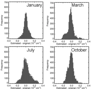
Fig. 3.Histograms of the difference between estimated and origi-nal stratospheric NO2columns over masked (polluted) areas based on simulated-data retrievals for January, March, July, and October 2005. Each histogram has a 2-sigma level deviation of approxi-mately 0.2×1015cm−2.
the CTM tropospheric vertical column, (2)σSAtrop
trop are a priori Stroperrors due toAtrop, and (3)σδVstrat are stratospheric in-terpolation errors in the masked regions (see Sect. 4.1.2). We write the combined variance as
(σVstrat)
2=(σCTM
Strop /Astrat)
2+(σAtrop Strop /Astrat)
2+(σ
δVstrat)
2. (22)
Although the CTM errors are not known, we estimate the uncertainties from sources (1) and (2) (first two terms) to be approximately 50 %. Therefore, by Eq. (10), with
ε= 0.3×1015cm−2, these errors are <0.15×1015cm−2 each. The third term in Eq. (22) applies only to masked areas (see Sect. 4.1.2). An estimate of its value was ob-tained from an analysis of simulated data. Using the monthly mean GMI model NO2profiles and daily views of geometry, pressure, reflectivity, and cloud parameters from OMI, a set of simulated slant-column measurements was constructed. The STS algorithm was then applied to these slant columns and the retrieved stratospheric vertical columns were com-pared to those of the original model. Histograms of the stratospheric errors in the masked regions for four months are shown in Fig. 3, which indicates 1σ errors of approx-imately 0.1×1015cm−2. Therefore, the combined strato-spheric vertical-column error computed from Eq. (22) is on the order of 0.2×1015cm−2. Errors in masked (polluted) re-gions can be slightly larger than this value, while errors in the cleanest areas (e.g., high-latitude, unpolluted areas) are typi-cally significantly smaller. The use of 0.2×1015cm−2as an approximate value for stratospheric uncertainty is consistent
Fig. 4.Mean tropospheric NO2 vertical-column errors (solid
cir-cles) as a function of cloud radiance fraction, based on SP2 data from 21 March 2005. Vertical lines show error standard deviations and open circles indicate median values.
with previous estimates by Boersma et al. (2004) and Buc-sela et al. (2006). The masking threshold of 0.3×1015cm−2 was chosen, in part, to make the total stratospheric vertical-column uncertainty close to this value. Section 4.1 offers fur-ther discussions of the effects of errors associated with the STS algorithm.
3.3 Vertical-column errors
The uncertainties in the retrieved vertical-column amounts are calculated by treating the uncertainties inS,Vstrat,Astrat, andAtropas independent. Based on the definitions of tropo-spheric and total columns in Eqs. (11) and (12), this assump-tion yields the following variances in the tropospheric and total vertical columns:
σV2
trop=
h
σS2+(Astrat·σVstrat)
2+ (23)
(Vstrat·σAstrat) 2+(V
trop·σAtrop) 2i/A2
trop
and
σV2=σV2
trop+σ
2
Vstrat·(1−2·Astrat/Atrop), (24)
4 Discussion and comparisons with other datasets
The main components that distinguish the SP2 algorithm from SP1 and other satellite NO2retrieval schemes involve the STS and tropospheric air mass factors. In this section, we further examine the STS algorithm, compare with OMI retrievals from other algorithms, and re-examine validation using in situ measurements.
4.1 Retrieval effects of a priori assumptions in the STS algorithm
The a priori tropospheric NO2columns and the masking, in-terpolation, and smoothing components of the STS algorithm affect NO2 retrieval accuracy. In general, over the cleanest areas (open-ocean and high-latitude regions), the SP2 algo-rithm yieldsVstratvalues that are approximately as accurate as the NO2slant columns and contain only small amounts of a priori model information from the tropospheric climatol-ogy. Relatively little independent tropospheric information is retrieved from these regions, but local enhancements rel-ative to the a priori troposphere can be observed. The re-trieval over clean regions consists of small-scale (smaller than ∼3◦) tropospheric features and measurement noise. Over polluted (masked) regions, the SP2 algorithm provides
Vtropretrievals that are mainly dependent on the assumed lo-cal profile shapes and surface reflectivity climatology via the air mass factors.
Two scenarios in particular are challenging to the SP2 STS algorithm (and for nadir-viewing satellite retrievals in gen-eral). Firstly, over clean, unmasked regions, non-localized (broad) variations in tropospheric NO2relative to the a pri-ori climatology will necessarily appear as stratospheric NO2. Secondly, in polluted, masked areas, stratospheric features that depart significantly from the mean stratosphere in sur-rounding unmasked areas will be aliased into the tropo-spheric column. For example, a small-scale stratotropo-spheric en-hancement over a cloud-free polluted region on the US East Coast would be retrieved as a tropospheric enhancement. The inherent ambiguity in these scenarios can not be re-solved without additional information about the partitioning of stratospheric and tropospheric NO2.
To examine the behavior of the STS algorithm under such conditions, we consider idealized, noise-free retrievals over unmasked and masked regions. These are discussed and illus-trated in Sects. 4.1.1–4.1.3. For our simulations, we assume that the “true” stratospheric air mass factor,Astrat, is equal to its a priori estimate,Astrat, and is invariant on scales smaller than the widths of the smoothing windows: <Astrat>≈Astrat (on this scale we ignore the effects of viewing geometry). In this discussion, we use an overline for variables to represent “true” (as opposed to a priori) atmospheric values, brackets <>to indicate window averages, and a prime (′)to designate values in masked (polluted) areas.
4.1.1 Retrievals in unmasked (clean) regions
If the measured slant column is the sum of the true strato-spheric and tropostrato-spheric slant columns, S=Sstrat+Strop, then it can be shown from Eq. (9) that the retrieved strato-spheric vertical column in unmasked (clean) regions is given by
Vstrat_RET=< Vstrat>−(< Strop>−< Strop>)/Astrat, (25)
where< Vstrat>is the window-averaged true stratospheric vertical column. Equation (25) states that the retrieved spheric vertical column is the average of the true strato-spheric vertical column plus an error term from the difference between the true and a priori tropospheric slant columns. When the a priori tropospheric slant column is correct and the true stratospheric field is smooth on the scale of the smoothing window, then the stratospheric retrieval is unbi-ased:Vstrat_RET≈Vstrat.
If the true stratospheric field is homogeneous within the averaging window from Eq. (11), then the retrieved tropo-sphere in unmasked regions is
Vtrop_RET=Vtrop·(Atrop/Atrop)+(< Strop>−< Strop>)/Atrop. (26)
When the a priori tropospheric air mass factors are accurate (Atrop≈Atrop) and slowly varying, Eq. (26) becomes
Vtrop_RET≈< Vtrop>+(Vtrop−< Vtrop>). (27) Equation (27) shows that, in unmasked regions, the retrieved tropospheric vertical column is approximately equal to the a priori mean value (first term). However, the retrieval has ad-ditional fine-scale structure equal to the difference between the true tropospheric vertical column and its mean (second term).
4.1.2 Retrievals in masked (polluted) regions
The retrieved stratospheric vertical column in masked areas,
Vstrat_RET′ , is actually the interpolation-window average of the retrieved stratosphere in surrounding unmasked areas. We define the “true” stratosphere in masked areas as the similarly averaged true stratosphere from surrounding regions plus an amount,δVstrat, which varies from point to point inside the mask. The standard deviation ofδVstratisσδVstrat, which was derived in Sect. 3.2 from the histogram widths in Fig. 3. With these definitions, the tropospheric retrieval in a masked re-gion can be shown to be
Vtrop_RET′ =V′
trop·(A′trop/A′trop)+ (28)
(< Strop>−< Strop>)/A′trop+δVstrat·(A′strat/A′trop),
whereA′
stratandA′trop are the a priori stratospheric and tro-pospheric air mass factors in the masked area, andA′
tropis the true tropospheric air mass factor. As before, <Strop> and
Fig. 5.NO2vertical-column retrievals (red), using simulated data (black). The mean value of the tropospheric data (truth, black) was defined
to be larger than that of the algorithm’s a priori troposphere (blue). Shown are nadir pixels along two orbital segments:(a)and(c)are stratosphere and troposphere, respectively, for an unmasked segment in the eastern Pacific;(b)and(d)are stratosphere and troposphere, respectively, for a masked segment over eastern North America. In these simulations, geolocation, viewing geometry, and cloud parameters were taken from two orbits on 21 March 2005.
slant columns, respectively, in the surrounding unmasked ar-eas. We want our retrievalVtrop_RET′ to be as close as possible to the true troposphereV′
trop, and the three terms in Eq. (28) identify three possible sources of error. The first arises from potential mismatch of the true and a priori tropospheric air mass factors,A′
tropandA′trop. The true tropospheric vertical column will be scaled by their ratio. The second term shows errors due to the incorrect estimation of the a priori tropo-spheric slant columns in the surrounding areas. The third term describes tropospheric errors resulting from differences between the true stratosphere in the masked region and the mean stratosphere estimated from the surrounding regions. The second and third terms increase as the tropospheric air mass factor in the masked region (the denominator of each) decreases due to increasing aerosol or cloud fraction, for ex-ample. The result is that any biases caused by non-zero val-ues forδVstrator for <Strop> –< Strop>outside the mask will be amplified as the cloud fraction for a given pixel inside the mask increases. The bias is bounded, because measurements with large cloud fractions generally switch to the unmasked case described in Sect. 4.1.1.
4.1.3 Examples using simulated data
Figure 5 shows retrievals of simulated OMI slant-column data. The plots represent nadir pixels along sections of two OMI orbits, with viewing geometry and cloud parameters taken from the orbital data. In this simulation, we assume that all a priori air mass factors are correct, i.e., the true
air mass factors are the same as those used in the retrieval. Figure 5a and c illustrate stratospheric and tropospheric re-trievals, respectively, in an unmasked (clean) part of the east-ern Pacific. The retrieved stratospheric vertical column (red curve in Fig. 5a) is biased high because the simulated tropo-spheric data were intentionally made 50 % larger than the a priori troposphere in the unmasked regions. This bias affects the retrieved stratosphere via the second term in Eq. (25). Figure 5c shows the corresponding tropospheric retrieval. As expected from Eq. (27), the retrieval (red) follows the a priori (blue) rather than the true data (black), on average. However, it is evident that some of the smaller-scale differential struc-ture in the original data is preserved in the retrieval.
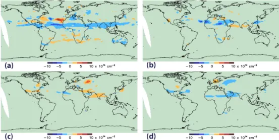
Fig. 6.Differences (= modified – nominal) in stratospheric field resulting from changes in masking threshold (nominal = 0.3×1015cm−2)
and interpolation window dimensions (see text) in the STS algorithm.(a)Tropospheric masking threshold decreased to 0.2×1015cm−2.
(b)Masking threshold increased to 0.4×1015cm−2.(c)Interpolation window halved in latitude and longitude width relative to nominal
size.(d)Interpolation window doubled in width.
Elsewhere, the tropospheric vertical column is slightly un-derestimated by an absolute amount comparable to that of the unmasked troposphere (Fig. 5c). As in the unmasked case, this underestimation is due to the error in the a priori tropo-sphere for the clean regions. The relative effect in this case appears small, since overall tropospheric columns are much larger in the masked region (note the difference in y-axis scaling for Fig. 5c and d).
In summary, the absolute stratospheric retrieval errors are generally small in most areas. The magnitude of the error de-pends on the magnitude of the bias between the a priori and true tropospheric fields. For OMI, we estimate that this bias introduces a stratospheric uncertainty of∼0.2×1015cm−2 or < 10 %. When tropospheric air mass factors are accurate, our simulations show that the absolute tropospheric vertical-column errors due to stratospheric errors are also small (on the order of 0.5×1015cm−2) in both masked and unmasked regions. The corresponding relative tropospheric errors in unmasked regions may be large due to the small tropospheric background amounts in those regions. Errors in tropospheric air mass factors will lead to proportional increases in both the absolute and relative tropospheric vertical-column errors in all areas.
4.1.4 Masking and interpolation sensitivity tests
The retrieved stratospheric field was examined for sensitiv-ity to parameters that control the initial masking and inter-polation in the STS algorithm. These steps are illustrated in Fig. 2d and e. We modified the masking threshold and the dimensions of the interpolation function (window) and computed the resultant stratospheric fields. In each case, the field based on the nominal parameters (see Sect. 2.4) was
subtracted from the modified field. The results, shown in Fig. 6, suggest that the retrieval is fairly robust with re-spect to the threshold and window dimensions. In Fig. 6a, the masking threshold was reduced from its nominal value of 0.3×1015 cm−2to 0.2×1015cm−2, and in Fig. 6b, the threshold was increased to 0.4×1015cm−2. The reduced threshold increases the number of masked pixels by a fac-tor of∼2, while the threshold increase approximately halves the masked-pixel count. The difference in the resultantVstrat is generally smaller than 0.5×1015cm−2 and is less than 0.1×1015cm−2over most of the Earth. The biggest effects are seen for the smaller threshold (0.2×1015cm−2), since this threshold results in more than half of Northern Hemi-sphere pixels being masked, leaving little data from which to accurately interpolate the stratospheric field. Tests involv-ing the interpolation algorithm are shown in Fig. 6c and d. In these figures, the latitude and longitude dimensions of the window were approximately halved and doubled, respec-tively. Results show that effects on the stratospheric field are even smaller than those seen in the threshold tests. We have also found that changing the shape of the interpolation func-tion (e.g., from boxes to circles) makes a negligible differ-ence in the resultant stratosphere.
4.2 Comparisons with other NO2retrieval algorithms and models
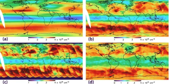
Fig. 7.Stratospheric NO2vertical-column retrieval for the date 21 March 2005.(a)SP1.(b)SP2.(c)DOMINO.(d)GMI (scaled to the
magnitude of SP2 using latitude-dependent scaling factors).
Fig. 8.Tropospheric NO2vertical-column retrieval for the date 21 March 2005.(a)SP1.(b)SP2.(c)DOMINO.(d)GMI. Note that all
negative values in SP1 were set to zero in the original SP1 public product. Also note that most of the negative values in the DOMINO product occur in cloudy or snow-covered regions and are flagged as unreliable.
sampled at the OMI overpass time and adjusted by empir-ical scaling factors to give approximate agreement in mag-nitude with the retrieved OMI stratosphere over the Pacific. The scaling factors were assumed to be linear functions of latitude and to vary between about 1.1 and 1.4. Linear vari-ation was assumed for simplicity only – the actual ratio be-tween the OMI and GMI stratospheres is more complicated, as evidenced by the discrepancy between the two strato-spheres (e.g., near the Equator). Nonetheless, a comparison of Fig. 7b and d shows that synoptic-scale structures in the model stratosphere are qualitatively similar to those retrieved by the SP2 algorithm. The stratosphere of the SP1 retrieval lacks structure on this scale and contains artifacts associ-ated with the wave-2 assumption in the SP1 retrieval.
Fig. 9.Monthly mean NO2comparisons of SP1 (blue), SP2 (red), and DOMINO (green):(a)January stratospheric zonal mean,(b)July
stratospheric zonal mean,(c)January NH troposphere (averaged over latitudes 35◦N to 55◦N),(d)July NH troposphere (averaged over latitudes 35◦N to 55◦N). In(c)and(d), the three regions of enhanced tropospheric NO2represent, from left to right, the USA, Europe,
and E. Asia, respectively. All measurements used for the tropospheric means were screened to exclude cloud radiance fractions greater than 50 %.
in Fig. 8. The tropospheric fields for all three OMI prod-ucts (Fig. 8a, b, and c) are qualitatively similar to the GMI March monthly mean field shown in Fig. 8d. The SP1 field shown in Fig. 8a has been recomputed using an off-line ver-sion of the SP1 algorithm that retains any negative values of tropospheric NO2. The SP2 tropospheric retrieval shows rel-atively few instances of negative tropospheric NO2compared to the other two OMI products. Monthly means from January and July (not shown) indicate that approximately 8 to 9 % of
Vtropcolumns retrieved from SP2 are significantly negative, defined here asVtrop<−0.2×1015cm−2. DOMINO tropo-spheric vertical columns have a somewhat higher frequency of negative values, and these occur predominantly in regions that are cloudy or snow-covered (and thus flagged as un-reliable). Approximately 21 % of the mostly cloudy (cloud radiance fraction > 0.5)Vtrop retrievals from DOMINO are significantly negative, compared to∼15 % of DOMINO re-trievals in relatively cloud-free regions. A comparison of Figs. 7c and 8c shows that some of the negative tropospheric values in DOMINO are associated with the strong cross-track variation in the DOMINO stratospheric field. Addi-tional comparisons among the three OMI data products may be found in the Supplement. Maps are shown in Figs. S1– S5, and statistical comparisons in the form of PDFs are given in Fig. S6. The figures provide further evidence of the rela-tive scarcity of negarela-tive tropospheric column amounts in SP2 compared to SP1 and DOMINO.
Larger-scale similarities and differences in the NO2 re-trievals can be seen by examining monthly means. Figure 9 compares monthly zonal means of stratospheric NO2in Jan-uary and July from SP1, SP2 and DOMINO, and the longitu-dinal variation of monthly mean tropospheric NO2in north-ern mid-latitudes for the same two months. In January and July, the stratospheric zonal means (Fig. 9a and b) are similar in all three products, with the SP2 slightly higher and the SP1 slightly lower than DOMINO. Larger differences are evident in the tropospheric means shown in Fig. 9c and d. Although the mean values of SP2 and DOMINO are similar (DOMINO is slightly lower in January and slightly higher in July at most longitudes), SP1 is consistently higher than SP2 by almost a factor of two in July. This discrepancy is likely due to the tropospheric air mass factors used in the SP1 retrieval, which did not account for the seasonal variability in NO2 profile shape (Lamsal et al., 2010).
4.3 Comparison with in situ measurements from INTEX-B
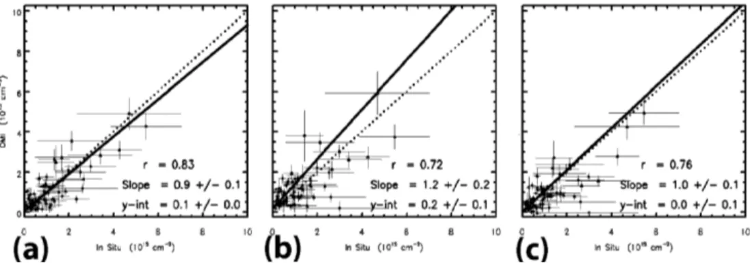
Fig. 10.Comparisons of tropospheric OMI NO2retrievals vs. integrated in situ LIF NO2measurements obtained during the INTEX-B field campaign over the Gulf of Mexico and clean Pacific locations. Shown are(a)SP1, but with collection 2 slant columns,(b)SP1 (current collection 3), and(c)SP2 (current collection 3). The solid line is an error-weighted least squares fit, and the dotted line is 1:1.
The INTEX-B campaign was conducted from March to May 2006 and included in situ data from the airborne Laser-Induced Fluorescence (LIF) instrument (Thornton et al., 2000, 2003), which measured NO2mixing ratios with an es-timated accuracy of ±10 % or ±5ppt. Mixing-ratio profiles were obtained at a number of locations in and near the Gulf of Mexico and parts of the Pacific Ocean. The former region included land measurements at polluted locations near Mex-ico City and Houston.
The LIF data were analyzed and compared by Bucsela et al. (2008), Boersma et al. (2008), and Hains et al. (2010) with OMI data. In the present study, we have employed a simi-lar approach to that of Bucsela et al. (2008). LIF data were selected for analysis based on the cloud/aerosol amount, al-titude range of the aircraft, and temporal (< 3 h) and spatial (< 20 km) proximity to the OMI overpass data. The profiles were integrated for comparison with OMI NO2tropospheric columns. All profiles required extrapolation in altitude, both above and below the actual measurements, to cover the full tropospheric column, and the amount of extrapolation was accounted for in the uncertainties assigned to each profile. Comparisons with OMI were made using x- and y-error weighted linear regression.
The following information describes our analysis of three different sets of OMNO2 data. The data are from (1) SP1 applied to collection 2 OMI data (as in the original study of Bucsela et al., 2008), (2) SP1 applied to collection 3, and (3) SP2 applied to collection 3. The collection 2 slant columns were retrieved from the OMI spectra based on pre-launch calibrations. Improved post-launch calibrations were used to construct a collection 3 dataset in 2007, as described by Dob-ber et al. (2008). All OMI examples shown previously in this study are based on collection 3 data. A summary of the com-parison results is shown in Fig. 10. In general, the agreement between the LIF and OMI data is good in all cases. Fig-ure 10a shows that the SP1 algorithm, using the original col-lection 2 OMI slant columns yields vertical columns slightly below those of the in situ LIF columns (see also Bucsela et
al., 2008). The regression OMI vs. in situ yields slope = 0.9,
y-intercept = 0.1×1015cm−2, and Pearson’s correlation co-efficient r=0.83. Using the collection 3 spectral radi-ances and the same SP1 algorithm (Fig. 10b), we obtain slope = 1.2, y-intercept = 0.2×1015cm−2, and r= 0.72, re-spectively. This result implies a modest overestimate of NO2 by OMI relative to the in situ measurements. Figure 10c shows the reanalysis of the same collection 3 data using the new SP2 algorithm. In this case, the slope and intercept are approximately unity and zero, respectively, and the corre-lation coefficient isr= 0.76. The slope and intercept in the latest OMNO2 dataset indicate the best agreement with the INTEX-B data of the three comparison figures. Although this analysis was based on springtime rather than summer-time data, the smaller tropospheric columns in SP2 relative to SP1 (for the same collection 3 dataset) appear consistent with Fig. 9d and the results of Lamsal et al. (2013).
5 Summary and conclusions
of small additional errors in the stratospheric field. The ef-fect on the retrieved stratosphere of modest changes in the interpolation parameters (e.g., the extent of masking or the interpolation-window size and shape) is relatively small.
Tests using simulated data show reasonable accuracy in the OMI SP2 retrievals, with clear-sky tropospheric errors over most regions on the order of∼1015cm−2. Recent validation studies comparing OMNO2 SP2 with independent measure-ments also suggest improvement over SP1-based validations. We note fewer instances of negative tropospheric vertical columns relative to SP1 and the DOMINO product. How-ever, the general agreement between OMNO2 and DOMINO has improved with the introduction of the SP2 algorithm. This agreement is noteworthy, given the very different STS algorithms used in the two products. The discrepancies be-tween polluted summertime tropospheric vertical columns from OMI and those from independent measurements have been greatly reduced in SP2 compared to SP1 and are also small relative to DOMINO.
The quality of the SP2 data is currently being established by independent measurements in ongoing validation cam-paigns from ground, aircraft, and satellite instruments. Better error estimates in the SP2 product should facilitate the com-parisons, and future work will help to refine the error esti-mates. Differences in the behavior of the SP2 algorithm un-der clear/cloudy, polluted/clean, and masked/unmasked con-ditions should also be kept in mind when comparing OMI datasets. Versions of the SP2 algorithm are also planned for testing with data from other satellite instruments, including SCIAMACHY, GOME-2 and TROPOMI.
Supplementary material related to this article is available online at http://www.atmos-meas-tech.net/6/ 2607/2013/amt-6-2607-2013-supplement.pdf.
Acknowledgements. We acknowledge the NASA Earth Science Division for funding of the OMI Standard NO2product
develop-ment and analysis. The Dutch-Finnish-built OMI instrudevelop-ment is part of the NASA EOS Aura satellite payload. The OMI instrument is managed by KNMI and the Netherlands Agency for Aerospace Programs (NIVR). The authors also wish to thank the editor and referees for their helpful comments in preparing this paper.
Edited by: M. Weber
References
Acarreta, J. R., deHaan, J. F., and Stammes, P.: Cloud pressure re-trieval using the O2-O2absorption band at 477 nm, J. Geophys.
Res., 109, D05204, doi:10.1029/2003JD003915, 2004. Bass and Johnsten, World Meteorological Organization, 1975. Beirle, S., Platt, U., von Glasow, R., Wenig, M., and
Wag-ner, T.: Estimate of nitrogen oxide emissions from shipping by satellite remote sensing, Geophys. Res. Lett., 31, L18102, doi:10.1029/2004GL020312, 2004.
Beirle, S., Kuhl, S., Pukite, J., and Wagner, T.: Retrieval of tropo-spheric column densities of NO2from combined SCIAMACHY nadir/limb measurements, Atmos. Meas. Tech., 3, 283–299, doi:10.5194/amt-3-283-2010, 2010.
Beirle, S., Boersma, K. F., Platt, U., Lawrence, M. G., and Wag-ner, T.: Megacity Emissions and Lifetimes of Nitrogen Oxides Probed from Space, Science, 333, 1737–1739, 2011.
Bey, I., Jacob, D. J., Yantosca, R. M., Logan, J. A., Field, B. D., Fiore, A. M., Li, Q., Liu, H., Mickley, L. J., and Schultz, M. G.: Global modeling of tropospheric chemistry with assimilated me-teorology: Model description and evaluation, J. Geophys. Res., 106, 23073–23095, 2001.
Boersma, K. F., Bucsela, E. J., Brinksma, E. J., and Gleason, J. F.: NO2, in: OMI Algorithm Theoretical Basis Document, 4, OMI
Trace Gas Algorithms, ATB-OMI-04, Version 2.0, 20 edited by: Chance, K., 13–36, NASA Distrib. Active Archive Cent., Green-belt, MD, USA, August 2002.
Boersma, K. F., Eskes, H. J., and Brinksma, E. J.: Error analysis for tropospheric NO2from space, J. Geophys. Res., 109, D04311,
doi:10.1029/2003JD003962, 2004.
Boersma, K. F., Eskes, H. J., Veefkind, J. P., Brinksma, E. J., van der A, R. J., Sneep, M., van den Oord, G. H. J., Levelt, P. F., Stammes, P., Gleason, J. F., and Bucsela, E. J.: Near-real time retrieval of tropospheric NO2from OMI, Atmos. Chem. Phys.,
7, 2103–2118, doi:10.5194/acp-7-2103-2007, 2007.
Boersma, K. F., Jacob, D. J., Bucsela, E. J., Perring, A. E., Dirksen, R., van der A, R. J., Yantosca, R. M., Park, R. J., Wenig, M. O., Bertram, T. H., and Cohen, R. C.: Valida-tion of OMI tropospheric NO2 observations during INTEX-B
and application to constrain NOx emissions over the eastern
United States and Mexico, Atmos. Environ., 42, 4480–4497, doi:10.1016/j.atmosenv.2008.02.004, 2008.
Boersma, K. F., Eskes, H. J., Dirksen, R. J., van der A, R. J., Veefkind, J. P., Stammes, P., Huijnen, V., Kleipool, Q. L., Sneep, M., Claas, J., Leitão, J., Richter, A., Zhou, Y., and Brunner, D.: An improved tropospheric NO2 column retrieval algorithm for
the Ozone Monitoring Instrument, Atmos. Meas. Tech., 4, 1905– 1928, doi:10.5194/amt-4-1905-2011, 2011.
Bovensmann, H., Burrows, J. P., Buchwitz, M., Frerick, J., Noel, S., Chance, K. V., and Goede, A. P. H.: SCIAMACHY: Mission objectives and measurement modes, J. Atmos. Sci., 56, 127–150, 1999.
Brewer, A. W., McElroy, C. T., and Kerr, J. B.: Nitrogen diox-ide concentrations in the atmosphere, Nature, 246, 129–133, doi:10.1038/246129a0, 1973.
Bucsela, E. J., Celarier, E. A., Wenig, M. O., Gleason, J. F., Veefkind, J. P., Boersma, K. F., and Brinksma, E. J.: Algorithm for NO2 vertical column retrieval from the Ozone Monitoring Instrument, IEEE Trans. Geosci. Remote Sens., 44, 1245–1258, 2006.
Bucsela, E. J., Perring, A. E., Cohen, R. C., Boersma, K. F., Celarier, E. A., Gleason, J. F., Wenig, M. O., Bertram, T. H., Wooldridge, P. J., Dirksen, R., and Veefkind, J. P.: Comparison of tropospheric NO2from in situ aircraft measurements with near-real-time and
standard product data from OMI, J. Geophys. Res., 113, D16S31, doi:10.1029/2007JD008838, 2008.