Iodine monoxide in the Antarctic snowpack

(1)

ACPD

9, 25361–25407, 2009

IO in the Antarctic snowpack

U. Frieß et al.

Title Page

Abstract Introduction

Conclusions References

Tables Figures

◭ ◮

Back Close

Full Screen / Esc

Printer-friendly Version

Interactive Discussion

Atmos. Chem. Phys. Discuss., 9, 25361–25407, 2009 www.atmos-chem-phys-discuss.net/9/25361/2009/ © Author(s) 2009. This work is distributed under the Creative Commons Attribution 3.0 License.

Atmospheric Chemistry and Physics Discussions

This discussion paper is/has been under review for the journal Atmospheric Chemistry and Physics (ACP). Please refer to the corresponding final paper in ACP if available.

Iodine monoxide in the Antarctic

snowpack

U. Frieß1, T. Deutschmann1, B. Gilfedder2, R. Weller3, and U. Platt1

1

Institute of Environmental Physics, University of Heidelberg, Heidelberg, Germany

2

Institut f ¨ur Umweltgeologie, TU-Braunschweig, Germany

3

Alfred Wegener Institut f ¨ur Polar- und Meeresforschung, Bremerhaven, Germany

Received: 9 November 2009 – Accepted: 19 November 2009 – Published: 26 November 2009

Correspondence to: U. Frieß ([email protected])

(2)

ACPD

9, 25361–25407, 2009

U. Frieß et al.

Title Page

Tables Figures

◭ ◮

Back Close

Full Screen / Esc

Abstract

Recent ground-based and space borne observations suggest the presence of signif-icant amounts of iodine monoxide in the boundary layer of Antarctica, which are ex-pected to have an impact on the ozone budget and might contribute to the forma-tion of new airborne particles. So far, the source of these iodine radicals has been

5

unknown. This paper presents long-term measurements of iodine monoxide at the German Antarctic research station Neumayer, which indicate that the snowpack is the main source for iodine radicals. The measurements have been performed us-ing multi-axis differential optical absorption spectroscopy (MAX-DOAS). Using a cou-pled atmosphere-snowpack radiative transfer model, the comparison of the signals

10

observed from scattered skylight and from light reflected by the snowpack yields sev-eral ppb of iodine monoxide in the upper layers of the sunlit snowpack throughout the year. Snow pit samples from Neumayer Station contain up to 700 ng/l of total iodine, representing a su_fficient reservoir for these extraordinarily high IO concentrations.

1 Introduction

15

It is known since the mid 1980s that a strong enrichment in iodine is present in coastal areas of Antarctica. Evidence came from analysis of meteorites collected on the shelf ice of Antarctica (Dreibus and W ¨anke, 1983). Extremely high iodine concentrations of 11-15 ppm were measured in Antarctic meteorites, whereas the mean iodine content in non-Antarctic meteorites of the same type was only 0.07 ppm (Dreibus et al., 1979).

20

Later, Heumann et al. (1987) analysed meteorites, rock samples, snow and aerosols near the Antarctic coast. They found more than 1 ppm of iodine in meteorites and I/Cl ratios in snow samples 10–190 times higher than in sea water, but no or only small enrichment in chlorine and bromine. Rock samples showed a decrease of the iodine – but not bromine and chlorine – concentration from the surface to the centre of

25

(3)

ACPD

9, 25361–25407, 2009

U. Frieß et al.

Title Page

Tables Figures

◭ ◮

Back Close

Full Screen / Esc

surfaces of Antarctic rocks. This finding was confirmed by halogen depth profiles in Antarctic chondrides, which showed an enrichment in iodine at the surface not present in samples anywhere else in the world (Langenauer and Kr ¨ahenb ¨uhl, 1993). Heumann et al. (1987) concluded from the lack of iodine enrichment in aerosol samples that iodine must be transported from the coast to inland Antarctica in gaseous form as

5

organoiodides (e.g., methyl iodide with a lifetime of ≈5 days), since the lifetime of inorganic iodine compounds (e.g., I2 and HI) was too short to explain the iodine high

abundance o_ffthe coast.

A possible mechanism for the release of gaseous iodine compounds from the ocean is the production of molecular iodine (I2) and hypoiodus acid (HOI) in the surface

sea-10

water by reaction of ambient ozone with iodide (Garland et al., 1980; Thompson and Zafiriou, 1983):

O₃+I−+H₂O→HOI+O₂+OH− (R1)

HOI+I−+H+→I2+H2O (R2)

The short-lived compounds I₂ and HOI subsequently react with dissolved organic matter in the seawater to produce iodinated organic compounds, such as CH3I, CH2I2,

CH2ICl, which escape to the atmosphere owing to their high volatility (Martino et al.,

15

2009). In particular methyl iodide (CH₃I), with a photochemical lifetime of several days, can be transported inlands before it is either deposed on the snow surface or photo-chemically destroyed to form reactive iodine compounds.

Iodine monoxide (IO) mixing ratios of several ppt have been detected by ground-based passive and active differential optical absorption spectroscopy (DOAS) (Frieß

20

et al., 2001; Saiz-Lopez et al., 2007b). Observations from satellite (Sch ¨onhardt et al., 2008; Saiz-Lopez et al., 2007a) indicate that the presence of IO is a widespread phe-nomenon along the Antarctic coast and over the sea ice covered Antarctic ocean.

The presence of iodine monoxide in the ppt range is expected to have a significant impact on the chemistry of the Antarctic boundary layer. It is expected to cause the

(4)

ACPD

9, 25361–25407, 2009

U. Frieß et al.

Title Page

Tables Figures

◭ ◮

Back Close

Full Screen / Esc

destruction of ozone via catalytic cycles involving the reaction of IO with a second halogen oxide molecule (BrO or IO) or with OH (Vogt et al., 1999; McFiggans et al., 2000):

2I+2O3→2IO+2O2 (R3)

IO+IO→2I+O2 (R4)

→OIO+I (R5)

→I₂O₂ (R6)

(R3) and (R4), as well as possible interhalogen reactions (i.e., IO+BrO) (Saiz-Lopez et al., 2007a), lead to the catalytic destruction of ozone. The branching ratio of OIO

5

formation via IO self reaction (R5) is≈40% (Bloss et al., 2001). There is much debate on the lifetime of OIO. The quantum yield for photolysis of OIO is small, and estimates of its lifetime range from several seconds to about one minute (Cox et al., 1999; Tucceri et al., 2006). Moreover, there is a debate on the product channels of OIO photolysis: Formation of O+IO would not lead to net ozone destruction, while I+O₂as products

10

would destroy ozone (Plane et al., 2006). The production of higher iodine oxides by polymerisation of OIO molecules possibly leads to the formation of new particles which may act as aerosol condensation nuclei (O’Dowd and Hoffmann, 2006) and might rep-resent a sink for reactive iodine. I2O2 is unstable and probably decays to regenerate

IO.

15

IO has not yet been detected in the Arctic, and it is yet unknown why this asymmetry exists and what the sources for the elevated levels of reactive iodine in Antarctica are. The emission of organoiodides (i.e., CH3I, CH2I2) by macroalgae and the subsequent

photodegradation of these compounds with photochemical lifetimes ranging between seconds and days has been identified as a source of reactive iodine coastal areas of

20

(5)

ACPD

9, 25361–25407, 2009

U. Frieß et al.

Title Page

Tables Figures

◭ ◮

Back Close

Full Screen / Esc

a lifetime of only several minutes), or the direct emission of molecular iodine from sea-weed represents the main source for reactive iodine. In contrast, the presence of high amounts of iodine in Antarctica, both deposited on the surface and detected in reactive form form satellite far inland, suggests that long-range transport of iodine occurs via methyl iodide with a lifetime of several days.

5

This paper presents long-term measurements of IO by Multi-Axis DOAS in the Antarctic coastal region, performed at the German research station Neumayer II. By pointing the telescope not only upwards to the sky but also downwards on the snow surface, additional information on the trace gas distribution below the instrument and in the snowpack can be gained. The variation of the IO signal with elevation angle

10

can only be explained by large IO amounts in the snow interstitial, with mixing ratios of several ppb. Total iodine measurements in snowpit samples from Neumayer indicate that particulate iodine accumulated during winter is released to the gas phase during summer, representing a su_fficient source for the detected IO in the gas phase.

The instrumentation and the spectral analysis are described in Sects. 2 and 3,

re-15

spectively. The interpretation of the IO measurements the retrieval of vertical pro-file information requires the simulation of the coupled snowpack-atmosphere radiative transfer, which is subject of Sect. 4. The analysis of total iodine in snow pits collected at Neumayer Station is described in Sect. 5. Finally, the diurnal and seasonal varia-tion of the retrieved IO amounts in the atmosphere and snowpack and the total iodine

20

concentrations in snow pit samples are discussed in Sect. 6.

2 Instrumental

The DOAS instrument at Neumayer station (70◦S, 8◦W) has been continuously per-forming atmospheric trace gas measurements since January 1999. Neumayer II (which has been replaced by the new station Neumayer III this summer) was located on the

25

(6)

ACPD

9, 25361–25407, 2009

U. Frieß et al.

Title Page

Tables Figures

◭ ◮

Back Close

Full Screen / Esc

bay in north-eastern direction.

The Neumayer DOAS instrument has already been described in detail elsewhere (Ferlemann et al., 2000; Frieß et al., 2001; Frieß et al., 2004) and is therefore only briefly described here. It consists of two separate spectrograph-detector units consist-ing of holographic concave gratconsist-ings and photodiode arrays cooled to−30◦C to minimise

5

dark current and detector noise. The instrument covers the wavelength regions of 320 to 420 nm (UV) and 400 to 650 nm (Vis) with a spectral resolution of approximately 0.5 and 1 nm, respectively. The optical benches of the spectrometer units, made of 5 mm stainless steel plates, are mounted inside a temperature stabilised, vacuum sealed alu-minium vessel, filled with dry argon. The instrument is characterised by an excellent

10

stability, which is crucial for high-quality long-term measurements.

Scattered skylight from the telescope unit is fed to the spectrometers using depolar-ising quartz fibre bundles. Initially, only zenith-sky measurements were performed, until the telescope unit was replaced by a multi-axis telescope in austral summer 2003. It is equipped with two prisms, each mounted on the axis of a stepper motor. This set-up

al-15

lows for varying the elevation angleα(the angle between zenith and viewing direction). Skylight is reflected by the prisms at an angle of 90◦ and focused on the entrances of the fibre bundles by plano-convex lenses. The entrance optics are located inside a quartz glass tube of 145 mm diameter, which is integrated into a heated stainless steel housing. The entrance optics has a field of view (FOV) of 1◦. The telescope is mounted

20

on the roof of the Neumayer trace gas observatory, at a height of approximately 7 m over the snow surface. The viewing plane of the telescope is directed to the north.

UV and Vis spectra are recorded with a total integration time of 3 min during the day, at solar zenith angles (SZA) of θ<90◦. During twilight, the integration time in-creases to up to 800 seconds atθ=97◦. Only zenith sky measurements are performed

25

(7)

ACPD

9, 25361–25407, 2009

U. Frieß et al.

Title Page

Tables Figures

◭ ◮

Back Close

Full Screen / Esc

surface, are performed since 15 September 2007. These measurements contain in-formation on trace gases below the instrument and inside the snowpack, whereas the upward looking viewing directions are mainly sensitive for absorbers in the boundary layer above the instrument and, during twilight, in the stratosphere. The sensitivity of the measurements to the vertical distribution of trace gases will be discussed in detail

5

in Sect. 4.

Offset, dark current, as well as halogen- and mercury calibration spectra necessary for background correction, determination of instrument noise, wavelength calibration and monitoring of the spectral resolution, are recorded automatically each night.

3 Spectral analysis

10

The analysis of the spectra obtained by the Neumayer DOAS instrument is performed using the well established technique of differential optical absorption spectroscopy (DOAS) (Platt, 1994; Platt and Stutz, 2008). DOAS allows to determine the integrated concentration of atmospheric trace gases along the light path through the atmosphere, referred to as slant column density (SCD):

15

S=

ZL

0

ρ(s)d s (1)

with ρ_i(s) being the concentration of the trace gas at location s. Note that Eq. (1) is only a very simplified description the real processes in the atmosphere. In practice, the observed SCDs are the weighted average over a manifold of all possible light paths through the atmosphere, and the interpretation of the measurements requires the

simu-20

lation of the effective light path using a radiative transfer model (Marquard et al., 2000). The SCD depends on the observation geometry, i.e. on SZAθ, elevation angleα and relative solar azimuth angle (SAA)φ.

The SCDs of several absorbers are determined simultaneously using their individual absorption features as fingerprints. According to the Beer-Lambert law, the measured

(8)

ACPD

9, 25361–25407, 2009

U. Frieß et al.

Title Page

Tables Figures

◭ ◮

Back Close

Full Screen / Esc

optical density is given by

τmeas(λ)≡ −ln

_I

(λ)

Io(λ)

=

ZL

0

X

i

σ_i(λ)ρ(s)+k_r(λ,s)+k_m(λ,s) !

d s (2)

Here,σ_i(λ,T,p) is the temperature and pressure dependent absorption cross section of the ith trace gas, andk_r and k_m are the scattering cross sections for Rayleigh and

5

Mie scattering, respectively. I and I0 are spectra measured at different observation

geometries. For MAX-DOAS measurements, usually a zenith sky spectrum is chosen as referenceI0, whereasIis measured in off-axis geometry. Since trace gases are also

present when measuringI0, the spectral analysis yields the differential slant column

density (dSCD)d S=S−Sref.

10

The DOAS method uses the fact thatk_randk_monly vary slowly with wavelength and can be approximated by a polynomial of appropriate orderN, whereas the absorption cross sectionsσi contain high frequency structures, acting as individual fingerprints for

the detection of trace gases. In the spectral analysis procedure, the optical depth is modelled according to

15

τmodel(λ)=

X

i

σ_i(λ)S_i+

N

X

n=0

c_n λn (3)

Here σ_i are reference cross sections, usually measured in the laboratory and con-volved to the resolution of the spectrometer with the appropriate slit function. To ac-count for the temperature dependence of the cross sections, several reference spectra of the same trace gas at different temperatures can be included in the analysis.

20

(9)

ACPD

9, 25361–25407, 2009

U. Frieß et al.

Title Page

Tables Figures

◭ ◮

Back Close

Full Screen / Esc

least squares algorithm:

χ2≡ K₂

X

k=K₁

(τmeas(λk)−τmodel(λk))2→min (4)

Here λ_k is the centre wavelength of the kth detector pixel. The wavelength window of the retrieval, [λ(K1),λ(K2)], is chosen in order to optimise the signal-to-noise ratio of

the trace gases of interest, avoiding disturbing absorption features of other absorbers.

5

The residual root min square (RMS)χ quantifies the difference between measured and modelled optical depth and is a measure for the quality of the retrieval.

In the scope of this work, the analysis software Windoas (Fayt and van Roozendael, 2001) is used for the spectral analysis. In addition to the parameters Si and cn in

Eq. (3), Windoas supports a shift and squeeze of the pixel-to-wavelength mapping,

10

which compensates for possible changes in the instrument alignment, as well as a non-linear offset to the intensity, accounting for possible detector non-linearities and instrumental stray light.

The dispersion of the Vis spectrometer is determined by fitting a zenith sky spectrum recorded at noon to a high resolution Fraunhofer spectrum (Kurucz et al., 1984), which

15

has been convoluted with the measured mercury emission line at 435 nm.

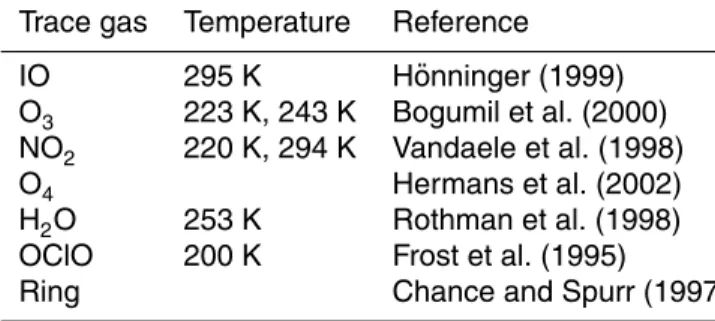
The retrieval of iodine monoxide is performed in the wavelength interval between 415 and 443 nm (corresponding to 140 detector pixels), encompassing three IO absorption bands. Apart from IO, the cross sections of ozone, NO2, O4, H2O and OClO are

included in the analysis. All cross sections are convolved with the Hg emission line

20

at 435 nm from a mercury lamp spectrum recorded by the Vis spectrometer. A Ring spectrum calculated according to Chance and Spurr (1997) accounts for the filling-in of the Fraunhofer lines by rotational Raman scattering (Grainger and Ring, 1962). A third order polynomial accounts for the broad band spectral features and a polynomial of second order is fitted as a non-linear intensity offset.

25

Two fixed Fraunhofer reference spectraI0, recorded at noon in zenith, were used for

(10)

ACPD

9, 25361–25407, 2009

U. Frieß et al.

Title Page

Tables Figures

◭ ◮

Back Close

Full Screen / Esc

of the spectra from July to December 2007, and from 17 February 2008 for the period of January to July 2008. The residual RMS of the IO analysis has a median of 8.2×10−5, but can be as low as 2.2×10−5and rarely exceeds 1.5×10−4during daytime.

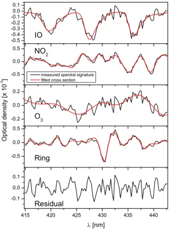
A typical example for the retrieval of IO at an elevation angle of 2◦is shown in Fig. 1. IO can be clearly detected, with a dSCD of (4.61±0.35)×1013molec/cm2

correspond-5

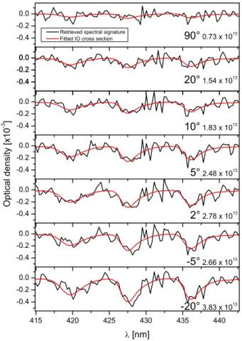
ing to a peak optical density of 4.8×10−4. The analysis residual has an RMS of only 6.2×10−5and a peak-to-peak optical density of 2.46×10−4. An example for the evolu-tion of the IO spectral signature under clear sky condievolu-tions as a funcevolu-tion of elevaevolu-tion angle is shown in Fig. 2. An increase with decreasing elevation angle is observed, with the highest IO dSCD measured when pointing the telescope downwards on the snow

10

surface at−20◦elevation angle. The Fraunhofer calcium line causes some increase in the residual structure around 430 nm, which can partly be explained by the decrease in intensity at the centre of the line causing higher photon noise.

In addition to IO, the oxygen collision complex O₄ at the 477 nm absorption band is retrieved in the wavelength interval between 450 and 500 nm using the same retrieval

15

settings as for IO, except that the absorption cross sections for IO and OClO are not included. Since the concentration of O₄ is proportional to the square of the oxygen concentration and is thus constant (apart from pressure and temperature variations), it is a useful indicator for changes in the light path, which can be caused by clouds or blowing snow. In fact, MAX-DOAS measurements of O₄ can be used to retrieve

20

information on atmospheric aerosols (Wagner et al., 2004; Frieß et al., 2006). Here O4is used to identify clear sky data as follows: The O4dSCDs are converted to

abso-lute SCDs by adding the reference SCD determined from a Langley plot based on O₄ measurements on a clear day. The measured SCDs are then compared to O4 SCDs

from a look-up table calculated by the McArtim radiative transfer model (see Sect. 4.2)

25

for a pure Rayleigh atmosphere. The look-up table contains simulated O₄ SCDs as a function of SZA, SAA and elevation angle. For each elevation angle sequenceα1.. αM,

(11)

de-ACPD

9, 25361–25407, 2009

U. Frieß et al.

Title Page

Tables Figures

◭ ◮

Back Close

Full Screen / Esc

termined according to

χ_O42 =

M

X

i=1

(S_O4meas(α_i)−S_O4model(α_i))2 (5)

Large χO4 values indicate that the atmospheric light path is altered by scattering

processes in clouds or blowing snow. The criterion χO4≤2×10 43

molec2cm−5 was found to be suitable for the identification of clear-sky conditions.

5

4 Radiative transfer in the atmosphere and snowpack

4.1 Qualitative discussion

The interpretation of MAX-DOAS measurements, and in particular the retrieval of infor-mation on the vertical profile of measured trace gases, requires the numerical simula-tion of the radiative transfer. The basic quantities to be modelled by a radiative transfer

10

model (RTM) which are necessary for profile retrieval are so-called box airmass factors (box-AMFs), which represent the sensitivity of the measured SCD to the partial vertical columns at different altitude layers:

a_{i j}=∂Si

∂v_j (6)

Here S_i is the SCD measured at elevation angle α_i (for the sake of simplicity, the

15

dependence on SZA and SAA are not considered in the following equations), and the partial vertical columnvj is the integrated concentration between altitude layerszj and z_j₊1:

v_j=

Zz_j₊₁

zj

(12)

ACPD

9, 25361–25407, 2009

U. Frieß et al.

Title Page

Tables Figures

◭ ◮

Back Close

Full Screen / Esc

For optically thin absorbers (such as IO), the box-AMFs do not depend on the vertical profile, and the SCDs can be calculated according to

S_i=X

j

a_{i j} v_j (8)

Conversely, Eq. (8) can serve as forward model for the retrieval of vertical profiles using the optimal estimation method (Rodgers, 2000).

5

The retrieval of vertical profiles from MAX-DOAS measurements has been subject of several publications (e.g., (Bruns et al., 2004; H ¨onninger et al., 2004; Wittrock et al., 2004; Sinreich et al., 2005; Frieß et al., 2006; Wagner et al., 2007)). However, ground-based MAX-DOAS measurements have so far only been discussed for conditions with low surface albedo. For observations above snow surfaces, the radiative transfer is

10

more complex and it needs to be considered that:

1. a significant amount of the observed scattered light has been reflected by the snow surface. Under clear sky conditions, the contribution of the upwelling radiation to the total (upwelling plus downwelling) radiation, as measured routinely by pyranometers at Neumayer, is approximately

15

45% (G. K ¨onig-Langlo, AWI Bremerhaven, personal communication, 2008, see http://www.awi.de/en/infrastructure/stations/neumayer station/observatories/ meteorological observatory/radiation measurements). Thus measurements at any viewing direction, not only when pointing the telescope downwards, are sen-sitive to trace gases below the instrument.

20

2. light hitting the snow surface enters the snowpack and is scattered many times un-til it leaves the snowpack again. Typical penetration depths of sunlight are several tens of centimetres (Lee-Taylor and Madronich, 2002). Thus scatted light mea-surements at any viewing direction are sensitive to trace gases in the uppermost layer of the snowpack.

(13)

ACPD

9, 25361–25407, 2009

U. Frieß et al.

Title Page

Tables Figures

◭ ◮

Back Close

Full Screen / Esc

A simplified sketch of this situation is depicted in Fig. 3. It is assumed that the trace gas is located in the planetary boundary layer, i.e. at altitudes below about 2 km. For the following discussion, the trace gas profile is separated into three layers: v_a

represents the partial VCD above the instrument (z > zinst), vb the partial VCD below

the instrument (0≤z≤zinst) andvs the partial VCD inside the snowpack (z<0).

5

For zenith-sky measurements (α=90◦, left panel of Fig. 3), the majority of direct sunlight (shown in yellow) is scattered into the line of sight (LOS) of the telescope (red line) in the upper troposphere and lower stratosphere, i.e. at altitudes above the trace gas layer. Thus, for surfaces with low albedo, the box-AMF for the layer above the instrument is close to one, whereas zenith-sky measurements are not sensitive for

10

trace gases below the instrument. The situation is di_fferent over snow surfaces since the large fraction of diffuse radiation that was in contact with the snowpack (blue line) makes zenith-sky measurements almost equally sensitive for trace gases below the instrument, and also sensitive for the snowpack.

Compared to zenith-sky measurements, off-axis measurements pointing above the

15

horizon (α>0◦, middle panel of Fig. 3) have a strongly enhanced sensitivity for trace gases above the instrument, which can be geometrically approximated by 1/sin(α). They also have an enhanced sensitivity for trace gases below the instrument and inside the snowpack, since the LOS is on average closer to the surface.

Direct sunlight contributes with 85% to the total downwelling radiation. Thus, mainly

20

directly reflected sunlight is observed when pointing the instrument downwards on the snow surface (α <0◦, right panel of Fig. 3). Therefore the box-AMF can be approxi-mated by 1/|sinα|+1/cosθfor the layer below the instrument, and by 1/cosθfor trace gases above the instrument. It is obvious that downward looking measurements are particularly sensitive for trace gases inside the snowpack, since the majority of the

de-25

(14)

there-ACPD

9, 25361–25407, 2009

U. Frieß et al.

Title Page

Tables Figures

◭ ◮

Back Close

Full Screen / Esc

fore be expected that, for downward looking viewing directions, the box-AMF for the snowpack has a dependency on the viewing direction weaker than 1/|sinα|.

However, high trace gas concentrations below the instrument and inside the snow-pack are necessary to cause a detectable signal. Given that the telescope of the Neu-mayer instrument is located at a height ofzinst=7 m above the snow surface, and with

5

a typical error of the IO dSCD of∆S=3.5×1012 molec/cm2, an average concentration below the instrument of ∆ρ_b=∆S/zinst×(1/|sinα|+1/cosθ)−

1

≈3.5×108 molec/cm2, corresponding to a mixing ratio of about 15 ppt, is required to cause a signal that ex-ceeds the retrieval error at an elevation angle ofα=−5◦and an SZA ofθ=70◦. Concen-trations inside the snowpack need to be even higher to be detectable, since radiation

10

penetrates the snowpack only down to some tens of centimetres.

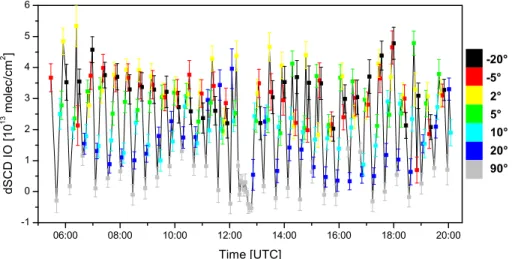
Now the findings of this qualitative discussion of the atmosphere-snowpack radiative transfer will be applied to measurements of IO at Neumayer. As an example, clear-sky IO dSCDs from 17 February 2008 are shown in Fig. 4. The IO dSCDs are characterised by the following features:

15

1. For viewing directions above the horizon (α>0◦), the IO dSCDs increase mono-tonically with decreasing elevation angle.

2. IO dSCDs from the downward viewing directions (−5◦ and −20◦) are of similar magnitude as the measurements at+2◦.

3. IO dSCDs at−20◦are similar to or even larger than those at−5◦.

20

Feature (1) can be caused both by IO located above and below the instrument. Fea-ture (2) indicates that a significant fraction of IO is located below the instrument (either in the atmosphere or inside the snowpack). Since the dSCDs do not vary proportional to 1/|sinα| for di_fferent downward viewing directions, the only explanation for feature (3) is that the majority of the detected IO is located inside the snowpack.

(15)

ACPD

9, 25361–25407, 2009

U. Frieß et al.

Title Page

Tables Figures

◭ ◮

Back Close

Full Screen / Esc

4.2 Radiative transfer modelling and profile retrieval

The coupled snowpack-atmosphere radiative transfer is modelled using the McArtim Monte Carlo radiative transfer model, which is the successor of Tracy 2 (Wagner et al., 2007; Deutschmann, 2008). It simulates an ensemble of photons in backward mode, i.e. photons are emitted from the telescope and their paths from the telescope to the

5

Sun is modelled. The box-AMFs (or in general weighting functions of atmospheric parameters) are computed as weighted means over the photon ensemble.

The model atmosphere is subdivided into layers of 100 m thickness up to an altitude of 3 km, and on a coarser grid up to 100 km. The lowermost layer extends from the snow surface up to an altitude of 7 m, which is the location of the telescope. Pressure

10

and temperature vertical profiles are adapted from a representative ozone sounding at Neumayer. No aerosols are included in the model atmosphere, which is justified by the good agreement between modelled and measured clear-sky O₄ dSCDs, confirming that the simulation of a pure Rayleigh atmosphere yields realistic results in this very clean environment.

15

For the simulation of the snowpack radiative transfer, a logarithmic height grid ex-tending down to a depth of 1 m is used. The thickness of the snow layers is 1 mm at the top, and is doubled for each following layer. The snowpack is basically treated as a very dense aerosol, using a Henyey-Greenstein phase function (Henyey and Green-stein, 1941). A snow extinction coefficient ofkm=6 cm−1has been adapted from King

20

and Simpson (2001), and single scattering albedo as well as asymmetry parameter are set toω=0.999982 andg=0.89 according to Lee-Taylor and Madronich (2002).

A lookup table of IO box-AMFs at λ=430 nm as a function of elevation angle, SZA and SAA has been calculated using an ensemble of 10 000 photons for each viewing geometry. Due to the large number of scattering events inside the snowpack, the

25

(16)

ACPD

9, 25361–25407, 2009

U. Frieß et al.

Title Page

Tables Figures

◭ ◮

Back Close

Full Screen / Esc

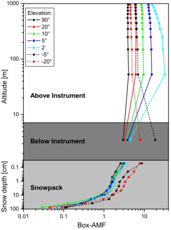
As expected, the box-AMFs for the atmosphere above the instrument strongly increase with decreasing elevation angle, from 4.1 in zenith to 32.4 at 2◦in the first 100 m above the telescope. Apart from the 2◦ viewing direction, the variation of the box-AMFs with altitude is weak, which implies that there is only limited information on the vertical profile above the instrument. Interestingly, downward viewing measurements have a higher

5

sensitivity for the atmosphere above the instrument than zenith-sky measurements, with box-AMFs of 7.0 and 5.0 for the−5◦and−20◦viewing directions, respectively.

Downward viewing directions are most sensitive for the atmosphere below the instru-ment, with box-AMFs of 18.7 and 7.9 for the−5◦and−20◦viewing directions, respec-tively. These values are significantly higher than calculated from the simple geometric

10

approximation discussed in Sect. 4.1 (14.2 and 5.8, respectively). The sensitivity of the upward looking viewing directions to the atmosphere below the instrument ranges from 3.0 in zenith sky to 4.4 at 2◦elevation.

For the uppermost 1 mm of the snowpack, box-AMFs of the downward viewing direc-tions are quite similar, with values of 8.7 and 7.7 for the−5◦and−20◦viewing directions,

15

respectively. The box-AMFs of the upward viewing directions for this thin layer of snow range between 2.6 (zenith) and 3.5 (2◦). However, the sensitivity of the MAX-DOAS measurements to trace gases in the snowpack quickly decreases with depth, with at-tenuation depths of the box-AMFs (i.e., the depth at which the box AMF reaches half of its surface value) ranging between 5 and 10 cm.

20

The box-AMFs calculated for the snowpack are subject of large uncertainties for several reasons. First, the statistical noise of the Monte Carlo simulations becomes very high in the lowermost snow layers owing to the small number of modelled photons reaching these depths. However, this is of minor importance since the contribution of light from deep snow layers to the observed signal is small. Second, the optical

25

(17)

ACPD

9, 25361–25407, 2009

U. Frieß et al.

Title Page

Tables Figures

◭ ◮

Back Close

Full Screen / Esc

The snow surface is treated as a horizontally and vertically homogeneous and flat layer. The topology of the snow surface, such as sastrugies and wind ripples which affect the radiative transfer, are not considered. Furthermore, snow properties vary seasonally owing to temperature variations and changes in morphology due to ageing processes, but also due to dispersion and deposition of snow crystals during blizzards.

5

The RTM also does not consider that the measurements, in particular at low elevation angle pointing northwards, are affected by light scattered both by the shelf ice and the sea ice due to the vicinity of Neumayer station to the ocean.

To retrieve the IO partial VCDsv_a,v_bandv_sintroduced in Sect. 4.1, the vertical reso-lution of the modelled box-AMFs is degraded to these three layers. A thickness of 1 km

10

is chosen for the layer above the instrument. Inside the snowpack, a box profile shape with a constant concentration down to a depth of 25 cm is assumed, corresponding to the typical penetration depth of radiation which can cause a photochemical production of IO.

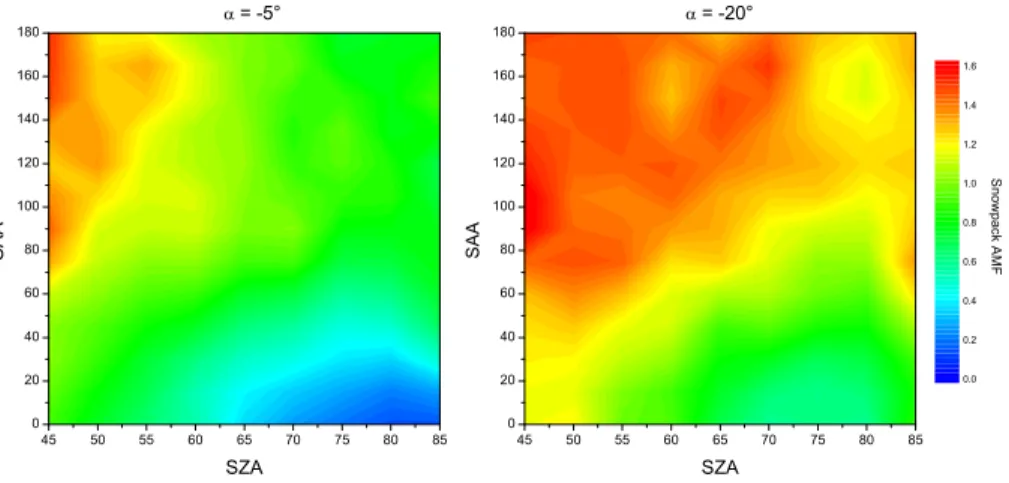
The resulting snowpack box-AMFs for the downward viewing directions are shown in

15

Fig. 6 as a function of SZA and SAA. Due to the averaging procedure with the assumed box profile as weight, the total AMFs for the snowpack are significantly smaller than the values at the surface from the height-resolved box-AMFs shown Fig. 5. As expected, the snowpack box-AMF for the−5◦viewing direction varies much stronger with viewing geometry than at−20◦elevation. In particular, the model predicts that measurements

20

at −5◦ are almost insensitive to trace gases in the snowpack at high SZA and SAA around zero, i.e. if the light hits the snow surface in a shallow angle and the instrument points towards the Sun. As already discussed above, this would only occur under ide-alised conditions if the snow surface would be completely flat. To account for variations of surface tilt due to sastrugis and wind ripples, a triangular smoothing is applied to

25

the snowpack box-AMFs which serve as weighting functions for the retrieval algorithm described in the following.

(18)

ACPD

9, 25361–25407, 2009

U. Frieß et al.

Title Page

Tables Figures

◭ ◮

Back Close

Full Screen / Esc

priori constraints are necessary, and the partial VCDs can be determined using a least squares algorithm, minimising the deviation between measured and modelled SCDs:

χ_R2≡(y−Kv)TS_ǫ−1(y−Kv)→min (9)

The estimate of the state vectorvˆ=( ˆv_a,vˆ_b,vˆ_s) is then given by ˆ

v=(KTS−_ǫ1K)−1(KTS−_ǫ1y) (10)

5

The vectory=(S₁,..,S_M) contains the measured IO SCDs at theM=7 different

view-ing angles of an elevation sequence, the elements of the weightview-ing functionKare the box-AMFs ai j, and the measurement error covariance Sǫ is a M×M matrix with the

square of the measurement errors as diagonal elements and the non-diagonal ele-ments set to zero. The retrieval error is represented by the covariance matrix of the

10

state vector:

ˆ

S=KTS−_ǫ1K (11)

For a retrieval based on differential instead of absolute SCDs, the weighting functions need to be replaced by differential box-AMFs, Ki j=ai j−a0j, by subtracting the

box-AMFs of the reference measurement atα0=90◦.

15

To enhance the accuracy of the retrieval, a two stage process is used. First, a retrieval is performed based on IO dSCDs with a fixed Fraunhofer reference spectrum. From the resulting partial VCDs, the according reference SCDs are calculated, and their error weighted average for clear sky conditions (determined using theχ_O4criterion as defined in Sect. 3) is added to the dSCDs, yielding absolute SCDs. In a final step,

20

partial VCDs are retrieved using absolute IO SCDs.

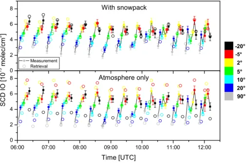
A comparison between measured and modelled IO SCDs is shown in Fig. 7. The upper panel shows the results for the standard retrieval with three layers, i.e. under the assumption that IO can be located above and below the instrument as well as in the snowpack. In this case, modelled and measured values are in good agreement and

25

(19)

ACPD

9, 25361–25407, 2009

U. Frieß et al.

Title Page

Tables Figures

◭ ◮

Back Close

Full Screen / Esc

model. A much poorer agreement between modelled and measured SCDs is achieved if the snowpack is excluded from the retrieval, i.e. if only two atmospheric layers above and below the instrument are retrieved and the snowpack concentration is set to zero. As shown in the lower panel of Fig. 7, in this case the model strongly underestimates the IO SCDs of the−20◦viewing direction, and the modelled+2◦and−5◦SCDs are too

5

high. This again illustrates that the measurements at Neumayer can only be explained if a significant fraction of the observed IO is located inside the snowpack. On the other hand, the retrieval is also not able to reproduce the measurements if IO is only retrieved below the instrument and inside the snowpack (not shown), indicating that there is a significant fraction of IO above the instrument as well.

10

Instead of the snowpack, IO could also be present in the atmosphere close to the snow surface, and multiple scattering inside blowing snow could lead to an amplification of the light path. To test this hypothesis, retrievals treating the snow surface as a Lambertian reflector (i.e., no IO inside the snowpack), and including a layer of blowing snow of 10–50 cm height above the surface, were performed with different extinction

15

coefficients of the blowing snow (1 m−1 and 3 m−1). These model runs were able to reproduce the measurements as well, yielding around 10 ppt of IO in the blowing snow layer. However, in this case the IO signal of the downward viewing directions should be below the detection limit at low wind speeds. Since no correlation between downward looking IO SCDs and wind speed has been observed, the hypothesis of an IO signal

20

from close to the surface, amplified by blowing snow, can be ruled out.

Similar agreement between measured and modelled IO dSCDs under clear sky con-ditions as shown in Fig. 7 has been achieved throughout the period of September 2007 to April 2008, except occasionally at low SZA when the Sun was located behind the instrument (θ≈180◦), i.e. around midnight in polar summer. Several sensitivity studies

25

(20)

ACPD

9, 25361–25407, 2009

U. Frieß et al.

Title Page

Tables Figures

◭ ◮

Back Close

Full Screen / Esc

cases, IO was detected inside the snowpack unambiguously.

4.3 Sensitivity on profile shape and snowpack extinction

The MAX-DOAS measurements of scattered light performed at Neumayer Station do not contain information on the IO profile shape inside the snowpack. However, the retrieved amount of IO inside the snowpack depends on the assumed profile shape,

5

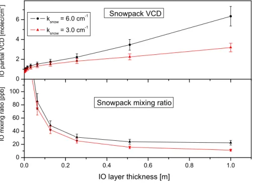
and also on the snow extinction coefficient. To investigate the sensitivity of the retrieval results on these parameters, a representative clear-sky measurement was chosen (2 February 2008, 11:00 UT), and retrievals were performed assuming a constant IO con-centration down to varying depths inside the snowpack. The resulting partial IO VCDs are shown in Fig. 8. Apart from the standard scenario with a snowpack extinction

co-10

efficient of 6 cm−1 (black lines), also calculations for half the extinction coefficient are shown (red lines).

The retrieved IO VCD inside the snowpack (upper panel of Fig. 8) increases with profile depth because the total snowpack AMF (the weighted sum of the box-AMFs, see Fig. 5) decreases and the VCD is given by the ratio between SCD and AMF. The lack

15

of sensitivity to layers below a certain depth leads to a linear increase of the snowpack VCDs for profile depths larger than≈25 cm. Thus the average mixing ratio (proportional to the ratio between VCD and profile depth) remains constant for profile depths larger than ≈25 cm, with values around 20 ppb (lower panel of Fig. 8). This value can be considered as a lower limit for the snowpack IO mixing ratio. The assumption of IO

20

being located only close to the surface would lead to unrealistically high mixing ratios, exceeding 100 ppb if the layer would be thinner than 5 cm. Thus the detected IO is likely to be located in the snow bulk rather than being concentrated in a thin layer close to the snow surface.

Since a decrease in snow density leads to an increase in penetration depth of light,

25

the retrieved IO mixing ratio is reduced to about half its value (about 10 ppb for a layer depth of 1 m) when halving the snowpack extinction coe_fficient (red line).

(21)

ACPD

9, 25361–25407, 2009

U. Frieß et al.

Title Page

Tables Figures

◭ ◮

Back Close

Full Screen / Esc

Neumayer can provide neither information on the partial IO VCD inside the snowpack nor on the IO mixing ratio, since both strongly depend on the assumed vertical profile inside the snowpack and on the snowpack optical properties. The results presented in Sect. 6 are based on the assumption that IO has a constant concentration profile inside first 25 cm the snowpack, and therefore provide only a rough estimate of the snowpack

5

IO VCDs and mixing ratios.

5 Analysis of total iodine from snow pit samples

A snow pit was excavated directly south of the Neumayer II research station during the austral summer 2008 field campaign of the Alfred Wegener Institute (AWI) (70.7137◦ S, 08.4179◦ W). The snow pit was 198 cm deep with samples being taken in

approx-10

imately 5 cm intervals and stored in clean Nalgene polypropylene sample containers. All samples were transported frozen (−20◦C) to the AWI in Bremerhaven, Germany, and were measured for major cations and anions by ion chromatography. The samples were then refrozen and transported to Lake Constance (Germany) for measurement of total soluble iodine. The samples were allowed to warm to room temperature and, after

15

addition of187Re as internal standard, were measured by a Perkin Elmer Elan 6100 in-ductively coupled mass spectrometer peaking on the masses127I and79Br. Replicate measurements of selected samples were generally less than 10%, except when ap-proaching the detection limit (3σ=30 ng/l), where the relative standard deviation could be as high as 20–30%. The highest absolute error was±50 ng/l. The accuracy was

20

assessed by measuring standard reference material BCR-611 with the samples. The concentrations found were within the uncertainty of the certificate (indicative values only for iodine) and did not deviate from the average value by more than 10%. The snow density was measured in the field by weighing know volumes of snow/firn at each sampling point. Oxygen isotope data was measured at the AWI by Dr. Hans

25

(22)

ACPD

9, 25361–25407, 2009

U. Frieß et al.

Title Page

Tables Figures

◭ ◮

Back Close

Full Screen / Esc

6 Results and discussion

6.1 Iodine in snow pit samples

δ18O isotope signatures and the concentration of anions nitrate and methanesulphonic acid (MSA) were used to separate winter/summer snow accumulation periods in the snow profile. Theδ18O measurements provide an indication of the regional

tempera-5

ture, and thus a clear separation of Antarctic winter and summer during snow depo-sition. While some problems using δ18O as a seasonal tracer have been observed for low snow accumulation sites, high accumulation coastal areas such as Neumayer should give reliable data (Helsen et al., 2005). It is known from long-term aerosol and fresh snow measurements at Neumayer it that the concentration of nitrate and

10

MSA in aerosols show a strong seasonality with distinct maxima during austral sum-mer (Wagenbach, 1996). Nitrate and MSA formation are both dependent on photolytic processes, with MSA being a product of dimethyl sulphide oxidation by OH radicals dur-ing abstraction and addition oxidation pathways. It is thought that most of the nitrate excess (compared to background winter levels) observed during spring and summer

15

originates from sedimentation from the stratosphere. Thus these three independent indicators should give a reliable representation of summer/winter stratification in the snow pit, which can be clearly seen in Fig. 9. A similar approach has been applied by Hur et al. (2007) for trace metals in snow pits from .

As can be seen in Fig. 9, snowpack iodine concentrations in winter were relatively

20

low compared to snow at mid latitude sites (Gilfedder et al., 2008; Aldahan et al., 2009). However, iodine concentrations showed a high seasonal dependence, with significantly higher concentrations (up to 650 ng/l) in winter than in summer. Indeed, iodine con-centrations approached the detection limit during austral summer, and in some cases could not be detected at all. This points to efficient and significant iodine release from

25

(23)

ACPD

9, 25361–25407, 2009

U. Frieß et al.

Title Page

Tables Figures

◭ ◮

Back Close

Full Screen / Esc

(≈0.46 g/cm3), snow/firn iodine concentrations amount to 300 ng/l. If released directly into the gas-filled pore spaces, this would lead to≈95 ppbv of gas phase iodine. This is probably the absolute minimum amount of iodine that could be released from the snow pack, as the iodine concentrations in falling snow during spring and summer are likely to be somewhat higher than observed in winter, when biological productivity is

ex-5

pected to be at a minimum. For example, Heumann et al. (1987) observed a maximum iodine concentration in snow near Neumayer of 1800 ng/l.

A second observation that can be made from the clear seasonal trend in iodine snow pit data is that there must be very little vertical migration of iodine within the snow pack. If photolytic reactions were able to volatilise iodine at significant depths

10

(>5−10 cm), the iodine accumulated over winter would be released to the atmosphere. However, the obvious winter peak in iodine levels shows that iodine is only volatilised from the uppermost snow layers, with the iodine deposited in the winter accumulated snow remaining relatively stable.

6.2 Diurnal variation of IO

15

Partial IO VCDs above and below the instrument as well as in the snowpack, derived using the retrieval algorithm described in Sect. 4.2, are shown in Fig. 10 for a period of clear sky (1 to 4 February 2008).

Partial IO VCDs above the instrument (panel b) vary between

(1−4)×1012 molec/cm2. Assuming a uniform distribution of IO in a layer of 1 km

20

height, this corresponds to mixing ratios of only 0.4 to 1.6 ppt. The diurnal variation of IO above the instrument is characterised by a minimum around local noon, and slightly higher amounts in the evening than in the morning. This diurnal variation is similar to predictions from photochemical model calculations (Vogt et al., 1999), where the IO minimum at noon is caused by the reaction of HO₂ with IO to HOI, and the

25

am/pm asymmetry by a built-up of I2O2 by IO self reaction during the day. However,

(24)

ACPD

9, 25361–25407, 2009

U. Frieß et al.

Title Page

Tables Figures

◭ ◮

Back Close

Full Screen / Esc

modelled by Vogt et al. for mid-latitude conditions, and NO₂ concentrations around 3 ppt measured in the boundary layer at Neumayer (Jones et al., 1999; Jacobi et al., 2000) are likely to be too small to cause a significant formation of IONO2 during the

day. Another possible explanation for the noon minimum of IO above the instrument is a break-up of the boundary layer and a mixing in of free tropospheric air low in IO.

5

Inside the snowpack, IO VCDs of up to 5×1013molec/cm2are retrieved, with a mini-mum around noon which might be caused by the formation of HOI by reaction with HO₂. This corresponds to extremely high IO mixing ratios of up to 50 ppb inside the snow-pack (lower panel of Fig. 11). As discussed in Sect. 6.1, the snow pit measurements indicate that iodine accumulated in the particulate phase during winter is released to

10

the gas phase as soon as sunlight is available, leading to more than 100 ppb of iodine in the snow interstitial. Thus particulate iodine observed in the snow pit represents a sufficient reservoir to explain IO mixing ratios of≈50 ppb observed by MAX-DOAS.

However, from our current knowledge of iodine photochemistry, it is di_fficult to ex-plain how gas phase concentrations of IO in the order of several tens of ppb can

15

be sustained. Considering only gas phase chemistry, the lifetime of IO is lim-ited by self reaction, producing (instable) I₂O₂ and OIO. The latter has not been detected by MAX-DOAS. Given rate constants of 4.4×10−11cm3molec−1s−1 and 5.2×10−11cm3molec−1s−1 for reactions (R5) and (R6), respectively, the lifetime of IO would be less than 0.01 seconds, whereas the photolytic lifetimes of I₂O₂ and OIO

20

range between several seconds and 3 min. Possibly, I2O2 decomposes quickly to IO

by thermolysis (Vogt et al., 1999), and OIO can be converted to IO via reaction with NO (Pechtl et al., 2006), which is present in the snow pack at mixing ratios of up to 20 ppt. However, the high amounts of IO in the gas phase observed at Neumayer Sta-tion can most likely only be sustained by heterogeneous reacSta-tions on the snow surface.

25

In general, iodine recycling of intermediate iodine reservoir species (HOI, INO₂, INO₃ and I2O2) at the snow surface, proceeding via aqueous phase reaction with iodide, can

produce I2which is released back to the gas phase (for a comprehensive summary of

(25)

mecha-ACPD

9, 25361–25407, 2009

U. Frieß et al.

Title Page

Tables Figures

◭ ◮

Back Close

Full Screen / Esc

nisms leading to the direct conversion of OIO to IO are, however, not known. A possible mechanism proposed by Saiz-Lopez et al. (2008) is production of higher iodine oxides by OIO and a subsequent photolysis of I_xO_y.

The retrieved IO partial VCDs in the atmosphere between the snow surface and the instrument (panel c of Fig. 10) is characterised by a distinct diurnal variation with a

5

maximum of about 3×1012 molec/cm2 around noon. Distributed only over a height of 7 m, this corresponds to much higher concentrations than above the instrument, and it is likely that the majority of IO is located directly above the snow surface, as predicted by photochemical model calculations (Saiz-Lopez et al., 2008). Under the assumption that atmospheric and snowpack IO concentrations are equal at the

10

snow/atmosphere interface, an estimate for the IO layer height above the snowpack is calculated by dividing the partial VCD below the instrument (panel c of Fig. 10) by the snowpack IO concentration (lower panel of Fig. 11). The resulting IO layer height shown in the upper panel of Fig. 11 amounts to only a few centimetres. Simi-lar layer heights and snowpack/atmosphere gradients have been found for NO_x in the

15

sunlit snow/atmosphere interface at Summit/Greenland (Domin ´e and Shepson, 2002). Furthermore, a very strong gradient between snowpack and atmosphere has been observed for organohalogens (methyl bromide, ethyl- and methyl iodide) at Summit (Swanson et al., 2002), with a layer of up to 3.5 ppt of methyl iodide in the uppermost 10 cm of the snowpack and less than 0.3 ppt in the air, strongly suggesting

photochem-20

ical production mechanisms of these (and several other) compounds.

The IO partial VCD below the instrument correlates well with the snow temperature (red line in Fig. 11) determined from the routine pyrradiometer measurements at Neu-mayer under the assumption that snow represents a black body (G. K ¨onig-Langlo, per-sonal communication, 2008, http://www.awi.de/en/infrastructure/stations/neumayer

25

(26)

at-ACPD

9, 25361–25407, 2009

U. Frieß et al.

Title Page

Tables Figures

◭ ◮

Back Close

Full Screen / Esc

mosphere, whereas these transport processes are suppressed at high SZA owing to radiative cooling of the snow surface and a stable stratification of the boundary layer.

6.3 Seasonal variation of IO

Daily averaged partial IO VCDs are calculated including only clear-sky data as deter-mined by the O₄ measurements (see Sect. 3), and excluding retrievals which did not

5

converge (χ_R2>50, see Eq. 9). The resulting seasonal variation is shown in Fig. 12. No pronounced seasonal pattern of the partial IO VCDs above and below the instrument as well as in the snowpack is apparent, apart from a slight minimum of the IO amount inside the snowpack in late summer (January/February), and a decline in snowpack IO from mid March to April. In contrast to the MAX-DOAS IO observations, particulate

10

iodine measured inside the snowpack (Fig. 9) shows a strong seasonality. Concen-trations drop from up to 700 ng/l in winter down to almost zero in late summer, with a sharp gradient at the beginning and end of polar winter. This finding suggests that particulate iodine is quickly released to the gas phase as soon as sunlight is available. Note that the MAX-DOAS measurements were only performed during the day

15

(SZA<85◦), when a photochemical steady state between I and IO is already estab-lished (Vogt et al., 1999). Thus the IO VCDs averaged over 24 h, and therefore the total amount of reactive iodine released from the snowpack, are likely to be smaller as the amount of sunlight is decreased in early spring and late autumn.

The partial VCD below the instrument shows a large scatter, likely because the

sen-20

sitivity for the atmospheric layer below the instrument is very sensitive to perturbations of the light path by blowing snow, which can already occur at wind speeds of about 5 m/s. In case of blowing snow, the variation of the IO dSCDs with elevation angle will be reduced for the downward viewing angles, and the retrieval will attribute at least parts of the IO column above the snow surface to the snowpack.

25

(27)

interac-ACPD

9, 25361–25407, 2009

U. Frieß et al.

Title Page

Tables Figures

◭ ◮

Back Close

Full Screen / Esc

tions between bromine and iodine chemistry in polar spring can be drawn on the basis of the existing data, although somewhat higher IO partial VCDs below the instrument and inside the snowpack are retrieved in September 2007.

7 Conclusions

The MAX-DOAS measurements of iodine monoxide, together with total iodine

mea-5

surements from snow pits at Neumayer Station, suggest that the snowpack represents a strong source for iodine radicals in the boundary layer of coastal Antarctica. By in-cluding viewing directions not only pointing to the sky, but also downwards on the snow pack, the MAX-DOAS measurements can only be explained by the presence of huge amounts of IO in the snowpack interstitial air.

10

Using a retrieval algorithm on the basis of a coupled air/snowpack Monte Carlo radia-tive transfer model, snowpack IO concentrations can only be roughly estimated since the optical properties of the snowpack are not well known (and are likely to change with season), and the results strongly depend on assumptions on the depth of the IO layer inside the snowpack. Retrieved IO mixing mixing ratios in the range of 50 ppb

15

inside the snowpack are therefore subject to large uncertainties, and represent only an estimate of the order of magnitude. IO amounts above the snowpack (between snow surface and instrument) are comparatively small, and air highly enriched in IO is likely to be present only in a very thin layer of several centimetres height above the snow surface.

20

Total particulate iodine inside the snowpack shows a strong seasonal cycle, with maximum values of up to 650 ng/l in mid winter. Particulate iodine concentrations rapidly decrease as soon as sunlight is available during polar summer, indicating a pho-tochemically driven conversion to gaseous iodine compounds. The particulate iodine accumulated during winter corresponds to about 95 ppb of iodine in the gas phase, and

25

(28)

ACPD

9, 25361–25407, 2009

U. Frieß et al.

Title Page

Tables Figures

◭ ◮

Back Close

Full Screen / Esc

IO concentrations in the ppb range cannot be explained on the basis of our current knowledge of iodine chemistry, which predicts that IO concentrations should be limited by self reaction. The production of OIO should result in IO lifetimes of less than 0.01 s. It can only be speculated how such high IO amounts can be sustained: (1) the yield of OIO production is much smaller than currently estimated; (2) the photolytic lifetime of

5

OIO is very short; (3) higher iodine oxides, which might have a short photolytic lifetime, are quickly produced by OIO polymerisation; (3) there are unknown heterogeneous reactions on snow surfaces, leading to a fast re-conversion of OIO to IO.

Acknowledgements. This work has been financially supported by the German Research

Asso-ciation (DFG, project FR2497/2-1). Hans Oerter and Gert K ¨onig-Langlo from AWI are gratefully

10

acknowledged for providing the snow pit oxygen isotope data and meteorological data, respec-tively. Many thanks to the Neumayer over-winterer crews for operating and maintaining the long-term measurements at Neumayer for more than 10 years. Michel van Roozendael and Caroline Fayt from BIRA are gratefully acknowledged for providing the Windoas analysis pro-gram.

15

References

Aldahan, A., Persson, S., Possnert, G., and Hou, X. L.: Distribution of 127I and 129I in precipitation at high European latitudes, Geophys. Res. Lett., 36, L11805, doi:10.1029/ 2009GL037363, 2009. 25382

Alicke, B., Hebestreit, K., Stutz, J., and Platt, U.: Iodine oxide in the marine boundary layer,

20

Nature, 397, 572–573, doi:10.1038/17508, 1999. 25364

Allan, B. J., McFiggans, G., and Plane, J. M. C.: Observation of iodine monoxide in the remote marine boundary layer, J. Geophys. Res., 105, 14363–14369, doi:10.1029/1999JD901188, 2000. 25364

Bloss, W. J., Rowley, D. M., Cox, R. A., and Jones, R. L.: Kinetics and Products of the IO

25

Self-Reaction, J. Phys. Chem. A, 105, 7840–7854, doi:10.1021/jp0044936, 2001. 25364 Bogumil, K., Orphal, J., and Burrows, J. P.: Temperature-dependent absorption cross-sections

(29)

ACPD

9, 25361–25407, 2009

U. Frieß et al.

Title Page

Tables Figures

◭ ◮

Back Close

Full Screen / Esc

Bruns, M., Buehler, S., Burrows, J., Heue, K., Platt, U., Pundt, I., Richter, A., Rozanov, A., Wagner, T., and Wang, P.: Retrieval of profile information from airborne multiaxis UV-visible skylight absorption measurements, Appl. Opt., 43, 4415–4426, doi:10.1364/AO.43.004415, 2004. 25372

Carpenter, L. J., Sturges, W. T., Penkett, S. A., Liss, P., Alicke, B., Hebestreit, K., and Platt,

5

U.: Short-lived alkyl iodides and bromides at Mace Head, Ireland: links to biogenic sources and halogen oxide production, J. Geophys. Res., 104, 1679–1689, doi:10.1029/98JD02746, 1999. 25364

Chance, K. and Spurr, R. J. D.: Ring effect studies; Rayleigh scattering, including molecular parameters for rotational Raman scattering and the Fraunhofer spectrum, Appl. Opt., 36,

10

5224–5230, 1997. 25369, 25395

Cox, R. A., Bloss, W. J., and Jones, R. L.: OIO and the atmospheric cycle of iodine, Geophys. Res. Lett., 26, 1857–1860, doi:10.1029/1999GL900439, 1999. 25364

Deutschmann, T.: Atmospheric radiative transfer modelling using Monte Carlo methods, Diploma thesis, University of Heidelberg, Germany, 2008. 25375

15

Domin ´e, F. and Shepson, P. B.: Air-Snow Interactions and Atmospheric Chemistry, Science, 297, 1506–1510, doi:10.1126/science.1074610, 2002. 25385

Dreibus, G. and W ¨anke, H.: Halogens in Antarctic Meteorites, Meteoritics, 18, 291–292, 1983. 25362

Dreibus, G., Spettel, B., and W ¨anke, H.: Halogens in meteorites and their primordial

abun-20

dances, in: Origin and Distribution of the Elements, edited by: Ahrens, L. H., 33–38, 1979. 25362

Fayt, C. and van Roozendael, M.: Windoas user manual, IASB-BIRA, Brussels, Belgium, 2001. 25369

Ferlemann, F., Bauer, N., Fitzenberger, R., Harder, H., Osterkamp, H., Perner, D., Platt, U.,

25

Schneider, M., Vradelis, P., and Pfeilsticker, K.: Differential optical absorption spectroscopy instrument for stratospheric ballonborne trace-gas studies, Appl. Opt., 39, 2377–2386, 2000. 25366

Frieß U., Wagner, T., Pundt, I., Pfeilsticker, K., and Platt, U.: Spectroscopic measurements of tropospheric iodine oxide at Neumayer station, Antarctica, Geophys. Res. Lett., 28, 1941–

30

1944, 2001. 25363, 25366

(30)

ACPD

9, 25361–25407, 2009

U. Frieß et al.

Title Page

Tables Figures

◭ ◮

Back Close

Full Screen / Esc

109, D06305, doi:10.1029/2003JD004133, 2004. 25366

Frieß, U., Monks, P., Remedios, J., Rozanov, A., Sinreich, R., Wagner, T., and Platt, U.: MAX-DOAS O₄ measurements: A new technique to derive information on atmospheric aerosols: 2. Modeling studies, J. Geophys. Res., 111, D14203, doi:10.1029/2005JD006618, 2006. 25370, 25372

5

Frost, G. J., Goss, L. M., and Vaida, V.: Measurements of high-resolution ultraviolet-visible absorption cross sections at stratospheric temperatures 2. Chlorine dioxide, J. Geophys. Res., 101, 3879–3884, doi:10.1029/95JD03389, 1995. 25395

Garland, J. A., Elzerman, A. W., and Penkett, S. A.: The Mechanism for Dry Deposi-tion of Ozone to Seawater Surfaces, J. Geophys. Res., 85, 7488–7492, doi:10.1029/

10

JC085iC12p07488, 1980. 25363

Gilfedder, B. S., Lai, S. C., Petri, M., Biester, H., and Hoffmann, T.: Iodine speciation in rain, snow and aerosols, Atmos. Chem. Phys., 8, 6069–6084, 2008,

http://www.atmos-chem-phys.net/8/6069/2008/. 25382

Grainger, J. F. and Ring, J.: Anomalous Fraunhofer line profiles, Nature, 193, p. 762, 1962.

15

25369

Grenfell, T. C., Warren, S. G., and Mullen, P. C.: Reflection of solar radiation by the Antarctic snow surface at ultraviolet, visible, and near-infrared wavelengths, J. Geophys. Res., 99, 18669–18684, doi:10.1029/94JD01484, 1994. 25373

Helsen, M. M., van de Wal, R., van den Broeke, M., van As, D., Meijer, H., and Reijmer,

20

C.: Oxygen isotope variability in snow from western Dronning Maud Land, Antarctica and its relation to temperature, Tellus B, 57, 423–435, doi:10.1111/j.1600-0889.2005.00162.x, 2005. 25382

Henyey, L. C. and Greenstein, J. L.: Diffuse radiation in the Galaxy, Astrophys. J., 93, 70–83, 1941. 25375

25

Hermans, C., Vandaele, A. C., Fally, S., Carleer, M., Colin, R., Coquart, B., Jenouvrier, A., and M ´erienne, M. F.: Absorption cross-section of the collision-induced bands of oxygen from the UV to the NIR, in: NATO Advanced Research Workshop: Weakly Interacting Molecular Pairs: Unconventional Absorbers of Radiation in the Atmosphere, St. Petersburg, Russia, 2002. 25395

30