First space-borne measurements of the altitude distribution of mesospheric magnesium species

(1)

ACPD

7, 4597–4656, 2007

Mesospheric Mg species from space

M. Scharringhausen et al.

Title Page

Abstract Introduction

Conclusions References

Tables Figures

◭ ◮

Back Close

Full Screen / Esc

Printer-friendly Version

Interactive Discussion

EGU Atmos. Chem. Phys. Discuss., 7, 4597–4656, 2007

www.atmos-chem-phys-discuss.net/7/4597/2007/ © Author(s) 2007. This work is licensed

under a Creative Commons License.

Atmospheric Chemistry and Physics Discussions

First space-borne measurements of the

altitude distribution of mesospheric

magnesium species

M. Scharringhausen1, A. C. Aikin2, J. P. Burrows1, and M. Sinnhuber1

1

Institute of Environmental Physics, University of Bremen, Bremen, Germany 2

Institute for Astrophysics and Computational Sciences, The Catholic University of America, Washington, D.C., USA

Received: 9 January 2007 – Accepted: 26 March 2007 – Published: 2 April 2007

(2)

ACPD

7, 4597–4656, 2007

Title Page

Tables Figures

◭ ◮

Back Close

Full Screen / Esc

EGU Abstract

We present a joint retrieval as well as first results for mesospheric air density and mesospheric Magnesium species (Mg and Mg+) using limb data from the SCIAMACHY instrument on board the European ENVISAT satellite.

Metallic species like neutral Mg, ionized Mg+ and others (Fe, Si, Li, etc.) ablate

5

from meteoric dust, enter the gas phase and occur at high altitudes (≥70 km). Emis-sions from these species are clearly observed in the SCIAMACHY limb measurements. These emissions are used to retrieve total and thermospheric column densities as well as altitude-resolved profiles of metallic species in the altitude range of 70–92 km. In this paper, neutral Magnesium as well as its ionized counterpart Mg+ is considered. These

10

species feature resonance fluorescence in the wavelength range 279 and 285 nm and thus have a rather simple excitation process.

A radiative transfer model (RTM) for the mesosphere has been developed and val-idated. Based on a ray tracing kernel, radiances in a large wavelength range from 240–300 nm covering limb as well as nadir geometry can be calculated. The forward

15

model has been validated and shows good agreement with established models in the given wavelength range and a large altitude range.

The RTM has been coupled to a retrieval based on Optimal Estimation. Air density is retrieved from Rayleigh backscatter light. Mesospheric Mg and Mg+ number densities are retrieved from their emission signals observed in the limb scans of SCIAMACHY.

20

(3)

ACPD

7, 4597–4656, 2007

Title Page

Tables Figures

◭ ◮

Back Close

Full Screen / Esc

EGU 1 Introduction

The major source for metal species in the upper atmosphere is assumed to be influx of meteoric particles and cosmic dust. These particles enter the atmosphere at high velocities (12–72 km/s) and evaporate in the middle and upper atmosphere due to fric-tional heating with the ambient air.

5

The altitude of evaporation depends on the evaporation temperature of the species considered here. More volatile compounds ablate at higher altitudes. Table 1 gives an overview over evaporation points and approximative altitude ranges of maximum ablation of some species. Additionally, the relative abundances by mass in cosmic dust are given (abridged fromPlane,2003).

10

The ionic counterparts of the neutral metal species are formed by either charge transfer with nitrogen or oxygen or one of the ionization processes described below (see Sect.1.1).

At altitudes between 50 and 100 km, the intensity of solar radiation in the UV is strong, and thus the atmosphere is partly ionized. Equally, this altitude region can

15

be ionized by precipitating energetic particles from e.g. the sun. These particles are trapped within the radiation belts formed by the Earth’s magnetic field and precipitate to lower altitudes near the auroral ovals or the polar caps.

1.1 Chemistry of Mg and Mg+

In general, the following is true for all mesospheric metals: due to the high ionization

20

rate at high altitudes (above∼90 km), the dominant reactions and processes including metal species are determined by ion chemistry. At lower altitudes, major species for reaction with metal species are O, O₂, O₃, H, H₂ and H₂O, and the metals will form stable oxides or hydroxides as their dominant compounds (Plane,2003).

Magnesium is the metal species of highest meteoric abundance. Though the ionized

25

(4)

ACPD

7, 4597–4656, 2007

Title Page

Tables Figures

◭ ◮

Back Close

Full Screen / Esc

EGU the fact that ground-based measurement techniques (lidar, photometry) using the Mg

fundamental emission at 285 nm are impossible due to the strong ozone absorption in the Huggins bands at these wavelengths and lower altitudes.

Intense laboratory studies as well as model simulations have been undertaken (Plane and Helmer,1995) to estimate loss and production processes at respective altitudes.

5

The major loss reactions under consideration are oxidation and ionization:

Mg+_O₃_→_MgO+_O₂ ₍₁₎

Mg+_O₂+_N₂_→_MgO₂+_N₂ ₍₂₎

Mg+_hν(≤_162.2nm)_→_Mg+ ₍₃₎

Mg+_NO+ _→_Mg++_NO ₍₄₎

10

Mg+_O+

2 →Mg

+

+_O₂ ₍₅₎

Figure1shows the first-order loss rates of neutral magnesium in diff_{erent altitudes for} a December mid-latitude scenario. Despite some diurnal variability the dominant loss process below 95 km is Reaction (1). Photoionization as well as Reaction (2) play a minor role. The diurnal variations are due to variations in the rate of photoionization

15

(Reactions4,5) and photolysis (Reaction3).

Neutral Mg is mainly recovered by hydrogenolysis of a hydroxyl compound (Eq.8) as well as by oxidation of MgO (Eq.6). The ionic side of reaction pathways (Reactions9, 10) includes dissociative recombination of Mg+ oxides (Eqs.11,12):

MgO+_O_→_Mg+_O₂ ₍₆₎

20

MgO₂+_H_→_MgOH+_O ₍₇₎

MgOH+_H_→_Mg+_H₂_O ₍₈₎

Mg++_O₂+_M_→_MgO+

2 +M (9)

Mg++_O₃_→_MgO++_O₂ ₍₁₀₎

MgO++_e−_→_Mg+_O ₍₁₁₎

25

(5)

ACPD

7, 4597–4656, 2007

Title Page

Tables Figures

◭ ◮

Back Close

Full Screen / Esc

EGU The most stable neutral magnesium species is the dihydroxide Mg(OH)₂. It is formed

by reaction of an Magnesium oxide with water (Eq.13). The only destruction reaction to matter in the upper atmosphere is reaction with atomic hydrogen (which leads to recovery of neutral Mg (Eqs.14,8). Low number densities of atomic hydrogen on the one hand and increasing number densities of water vapour in lower altitudes on the

5

other hand make Mg(OH)2a very efficient reservoir species for Mg.

MgO+_H₂_O+_M_→_Mg(OH)₂+_M ₍₁₃₎

Mg(OH)2+H→MgOH+H2O (14)

We use SCIAMACHY limb measurements in an altitude region of 70–92 km to simul-taneously analyze Mg and Mg+ profiles. Thus, the partitioning as well as the spatial

10

variabilities of Mg and Mg+ can be investigated.

2 The SCIAMACHY instrument

The European ENVISAT satellite launched in March 2002 carries three instruments de-signed to perform observations of the atmosphere. Beside the Fourier transform spec-trometer MIPAS and the stellar occultation device GOMOS there is the SCIAMACHY

in-15

strument (ScanningImagingAbsorption Spectrometer forAtmosphericChartography). SCIAMACHY covers the wavelength range from 220 to 2380 nm with a spectral res-olution of 0.2 to 1.5 nm and provides nadir, limb and occultation viewing modes (Noel et al.,1999), see Fig.3. The limb viewing mode covers altitude levels from 0 to 92 km. This altitude range covers a large part of the mesosphere. Limb scans are used to

20

obtain altitude information of number densities, whereas the nadir mode provides total columns ranging from the ground to the exosphere.

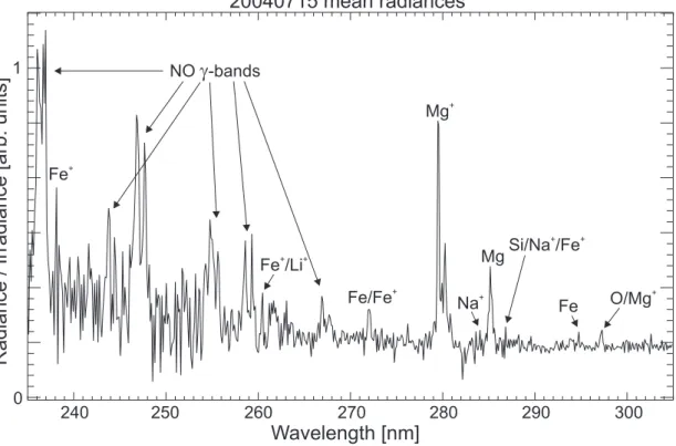
The SCIAMACHY wavelength range includes emission signals of several metallic and non-metallic species (Fig.4). Most emissions to be investigated in this study occur in the middle UV range. Beside emissions of the neutral species Fe, Mg and other

25

(6)

ACPD

7, 4597–4656, 2007

Title Page

Tables Figures

◭ ◮

Back Close

Full Screen / Esc

EGU the strong Na emission doublet at 589 nm can be observed easily in the SCIAMACHY

spectra. Oxygen species like O, O2, NO present some other prominent emission

fea-tures in the UV-Vis-NIR wavelength region.

3 Retrieval method

3.1 The forward model

5

3.1.1 Measurement geometry

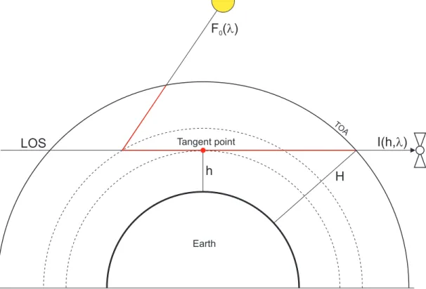
The SCIAMACHY instrument has three measurement modes (Sect.2): limb, nadir and occultation. We consider only the limb viewing mode where the line-of-sight (LOS) is parallel to a tangent of the Earth’s surface. Sunlight enters the atmosphere and gets scattered or absorbed. In case of absorption, radiation may be re-emitted e.g.

10

by resonance fluorescence. The instrument detects all radiation that is scattered or emitted into the LOS (Fig.5).

3.1.2 Basic assumptions

The SCIAMACHY instrument observes sunlight scattered and radiation emitted by the atmosphere. The number density of aerosols in the mesosphere is negligible and

15

thus – apart from noctilucent clouds – only Rayleigh scattering is presumed. Since the following considerations are restricted to applications within a wavelength range of 240–300 nm, all extinction is assumed to be due to ozone absorption in the Hartley-Huggins bands and Rayleigh single scattering out of the line-of-sight.

As multiple scattering in general increases the path length within the atmosphere, the

20

(7)

ACPD

7, 4597–4656, 2007

Title Page

Tables Figures

◭ ◮

Back Close

Full Screen / Esc

EGU scattering are neglected. The top-of-atmosphere is assumed to be atH=_{120 km. That}

is, the model assumes no atmosphere above this altitude.

All emissions considered are assumed to be due to resonance fluorescence. Self absorption of the emitters is accounted for.

It is assumed that the atmosphere is homogeneous horizontally as well as vertically

5

within a layer of thickness∆_{h. This value can be chosen by the user (see Sect.}_3.4). Though radiation emitted due to resonance fluorescence is unpolarized, the polariza-tion of Rayleigh scattering depends on the scattering angle. As SCIAMACHY consists of grid spectrometer devices, the radiation intensity detected depends on the polariza-tion of the light entering the instrument. This polarizapolariza-tion sensitivity of the instrument

10

is accounted for.

The radiative transfer model presented here will be denoted by MARS (Mesospheric Atmospheric Radiative Transfer Simulator). It has been compared to the radiative transfer model SCIARAYS (seeKaiser,2001). Results of limb calculations agree within 2.5% in an altitude range of 60–95 km, a wavelength range of 250–300 nm, and a range

15

of the solar angles of 0–88 for zenith and 0–180 for azimuth.

3.1.3 Rayleigh scattering and ozone absorption cross sections

We use the Cabannes form (Chandrasekhar,1960) of the Rayleigh scattering cross section for gaseous species. The following formula is slightly simplified according to the fact that the refractive index of the gaseous species under consideration is close to unity:

εRay(λ)=

32π3(ns−1)

2

3λ4_N2

L

(8)

ACPD

7, 4597–4656, 2007

Title Page

Tables Figures

◭ ◮

Back Close

Full Screen / Esc

EGU where the wavelength λ is given in nanometers, N_L=_2.69×1019_cm−3 _{denotes the}

Loschmidt number, andF_K is the King correction factor:

FK =

6+_3ρ

6−7ρ. (16)

Here,ρ is the depolarization factor of air. The commonly used valueρ=_{0.0295 (used} e.g. inRozanov,2001) is used in this radiative transfer model. The refractive index of standard airn_s is calculated using the Edl ´en formula (Edlen,1966):

n_s−1=

8342.13+ 2 406 030 130−106_λ−2 +

15 997 38.9−106_λ−2

×10−8 (17)

The Rayleigh phase scattering function is given by

P(θ)= 3 2(2+_ρ)

(1+_ρ)+₍₁₋_{ρ) cos}2_(θ)_, ₍₁₈₎

whereθdenotes the scattering angle (Eichmann,1995). The probability of scattering into a solid angledΩ_{under the scattering angle}_θ_{is given by}_P_(θ)dΩ_/4π.

Ozone absorption cross sections are taken from laboratory measurements (Burrows et al.,1999).

3.1.4 g-factors

5

The case of resonance fluorescence to the ground state is considered only. That is, the retrieval species are assumed to be excited by sunlight of wavelengthλ_{i j} from the ground statei to an energetically upper state j. De-excitation then leads to isotropic and unpolarized radiation of the same wavelength. Due to low number densities of all species considered here de-excitation by quenching is neglected.

10

The g-factor links number density and emitted radiance, e.g.

(9)

ACPD

7, 4597–4656, 2007

Title Page

Tables Figures

◭ ◮

Back Close

Full Screen / Esc

EGU Quantities indexed withi j correspond to the transition from the upper state j to the

lower statei. The g-factor is calculated as the product of the actinic flux, the absorp-tion cross secabsorp-tion σ_{i j} and the relative Einstein coeffi_{cient of spontaneous emission} (Anderson and Barth,1971). Here,σi j depends on the classical electron radius as well as on the transition wavelengthλi j and the oscillator strengthfi j. The relative Einstein

5

coeffi_{cient presents the probability of relaxation to the lower state} _i_{. Note that there} may be a number of lower states reachable from state j. This is accounted for by normalisingAi j by the sum of all respective absolute Einstein coefficients.

γi j =πF(λi j)·σi j· A_{i j}

P i′A_i′_j

(20)

=_πF_(λ_{i j}₎

| {z }

actinic flux

· πe

2

mc2fi jλ 2

i j | {z }

abs. cross section

· PAi j kAkj | {z }

rel. Einstein coeff_.

(21)

10

All values necessary for numerical calculations are obtained from the NIST database (NIST,2005).

3.1.5 Irradiance and radiance computations

(10)

ACPD

7, 4597–4656, 2007

Title Page

Tables Figures

◭ ◮

Back Close

Full Screen / Esc

EGU the absorption coeffi_cients_k_:

k(x, λ)=

nspecies_X

i=1

Ni(x)·σi(λ)=hN(x), σ(λ)i (22)

Using the Lambert-Beer’s law leads to the optical thicknessτsun, τsat(indexed withsun,

respectively. satto account for diff_{erent light paths from the sun to the scattering point} respectively. from the scattering point to the satellite). To calculate the solar irradiance F(Q, λ) present at a point Q within the atmosphere, it is necessary to integrate the absorption coeffi_{cient from}_Q _{to the TOA along the light path connecting the sun with}

5

Q:

F(Q, λ)=_F₀_(λ)_·_exp ₋

ZTOA

Q

k(s, λ)d s

!

(23)

=_F₀_(λ)_·_τ_sun_{(Q, λ)} ₍₂₄₎

A parameterization of the light path can be obtained by using the solar zenith and azimuth angleΦ_,Ψ_.

10

The conversion of irradianceF to radianceIis done by applying the Rayleigh phase functionP and the emissivity, respectively. the scattering cross section. As scattering and emission by resonance fluorescence are mathematically not distinguishable, the total emissivity can be written in a similar way as the absorption coeffi_cient:

E(Q, λ)=

nspecies_X

i=1

N_i(Q)·ε_i(λ)=_hN_{(Q), ε(λ)i} ₍₂₅₎

(11)

ACPD

7, 4597–4656, 2007

Title Page

Tables Figures

◭ ◮

Back Close

Full Screen / Esc

EGU atQ and the LOS. It depends on the local solar zenith angle as well as on the local

solar azimuth angle. Let the scattering angle be denoted byθQ. Note

θQ=θQ(Φ,Ψ) (26)

The light scattered in the LOS and entering the instrument is subject to extinction once again. The extinction betweenQand the instrument can be calculated analogously:

τsat(Q, λ)=exp −

Z+TOA

Q

hN(s), σ(λ)id s

!

(27)

Here,+_{TOA denotes the top-of-atmosphere towards the satellite.}

To obtain the total radiance at the instrument, the radiances at all pointsQalong the LOS have to be integrated and weighted with the respective optical thickness:

I(λ)=_F₀_(λ)_·

Z+TOA

−TOA

τsun(Q(s), λ)·E(Q(s), λ)·P(θQ(s))·τsat(Q(s), λ)d s

=_F₀_(λ)_·

Z+TOA

−TOA

τsun(s, λ)·E(s, λ)·P(s)·τsat(s, λ)d s (28)

5

Here,Q(s) denotes a parametrization of the LOS, and -TOA corresponds to the TOA away from the satellite. The second equation is a more convenient form of the first.

These integrals are evaluated by numerical quadrature using an adaptive grid (see Sect.3.4). That is, the atmosphere is divided into altitude layers and all quantities are evaluated at discrete locations along the respective light paths. The trapezoid rule is

10

used throughout the retrieval, as it is simple, fast and accurate at the same time. Let nsun, nsat, nLOS be the number of points the light paths are divided into. The

csun,i, csat,i, cLOS,i denote air mass factors (AMF) along the light paths, the discrete correspondences of the diff_{erential operators}_{d s:}

(12)

ACPD

7, 4597–4656, 2007

Title Page Abstract Introduction Conclusions References Tables Figures ◭ ◮ ◭ ◮ Back Close

Full Screen / Esc

EGU The following equations for the absorption coeffi_{cients and the total radiance hold:}

τsun(Q, λ)=exp

 −

n_sun+1

X

i=1

hN(si), σ(λ)icsun,i 

 (30)

τsat(Q, λ)=exp

 −

n_X_sat+1

i=1

hN(s_i), σ(λ)icsat, 

 (31)

I(λ)=_F₀_(λ)_· n_X_LOS

i=1

τsun(si, λ)·E(si, λ)·P(si)·τsat(si, λ)·cLOS,i (32)

5

3.1.6 Instrument simulator for limb geometry

In limb mode, the SCIAMACHY instrument performs 31 to 35 limb scans from the surface to≈92 km tangent altitude in steps of approx. 3.3 km. A last measurement is taken at 150–200 km, which is not included into the forward model. The instrument has a vertical field-of-view (FOV) of 2.6 km. Thus, the instrument convolves all radiation

10

within the FOV. This is accounted for by calculating the radiance on a fine altitude grid (stepsize 1 km) and then convolving the values with the SCIA FOV slit function of full-width-half-maximum (FWHM)W=_{2.6 km.}

For this purpose two slit functions have been tested. Rectangular:

S(h)=

0 ,|h| ≥W/2

1/W ,else (33)

Gaussian, order 10:

S(h)= 1

.9883W exp

"

−

2 ln(2)·h W

10#

(13)

ACPD

7, 4597–4656, 2007

Title Page

Tables Figures

◭ ◮

Back Close

Full Screen / Esc

EGU The standardization constant for the Gaussian is found using the following method: The

integralR∞_−∞S(h)dhis evaluated for a number of values for 1≤F≤10. The relationship between F and the value of the integral is virtually linear, and the integral vanishes forF=_{0. The regression coe}ffi_{cient is found to be between 1.068 and .9941, and the} relative error is well below .5% for all values ofF. This method has been tested for

5

Gaussians of order 2. . .20.

Diff_{erences between the results using di}ff_{erent slit functions are found to be small} and thus a Gaussian of order 10 is used throughout all calculations.

3.2 The retrieval

3.2.1 Basic principles

10

Taking into accountnal t altitude levels and nl amwavelengths, the observed limb ra-diances can be joined together in a measurement vector y. The same holds for the number density profiles of all species (remember that nspecies denotes the total num-ber of species), these are merged in anatmospheric state vectorx:

y ∈Rnlam·nalt , x∈Rnspecies·nalt (35)

The forward computations are treated in an analogous way using adiscrete forward model operatorF that depends on the atmospheric statex:

F :Rnspecies·nalt −→Rnlam·nalt (36)

However, due to discretization and other eff_{ects such as uncertainties in measuring the} observational parameters (SZA, altitude, etc) one has to allow for aforward errorδ:

y =_F_(x)+_δ ₍₃₇₎

(14)

ACPD

7, 4597–4656, 2007

Title Page

Tables Figures

◭ ◮

Back Close

Full Screen / Esc

EGU range ofF. That is, in general, Eq. (37) has no exact solution. Moreover, the altitude

resolution is limited as one limb view traverses the entire atmosphere. All altitudes above (and, due to the finite width of the field-of-view, to a certain extend even below) the tangent altitude contribute to the observed radiance. The latter is true even for a ideal measurement with no noise. Thus, the best one can do is to minimize

||y −F(x)||2

S_y−1, (38)

whereS_y denotes the measurement covariance matrix. This way, knowledge about the measurement uncertainties can be introduced as weighting factors in the retrieval. However, in general there is an infinite number of atmospheric state vectors x that minimize (38). Additionally, small perturbations of y due to noise may lead to large variations of the retrieval result. This may lead to large oscillations.

5

Thus, some kind of regularization has to be applied to restrict space of possible solutions. The most common regularization scheme is the Tikhonov regularization using a priori informationx_a:

||y −F(x)||2 Sy−1

+_||x₋_x_a_||2 Sa−1

→min (39)

Here,Sapresents thea priori covariance matrix. This matrix contains a priori uncertain-ties of the atmospheric parameters. This approach has been adapted and reformulated by C. Rodgers (seeRodgers,1976) to derive theOptimal Estimationmethod.

3.2.2 Weighting functions

The derivations of the limb radiances with respect to the atmospheric state parameters x_j constitute the weighting function matrixK:

Ki j = ∂F_i ∂xj

(15)

ACPD

7, 4597–4656, 2007

Title Page Abstract Introduction Conclusions References Tables Figures ◭ ◮ ◭ ◮ Back Close

Full Screen / Esc

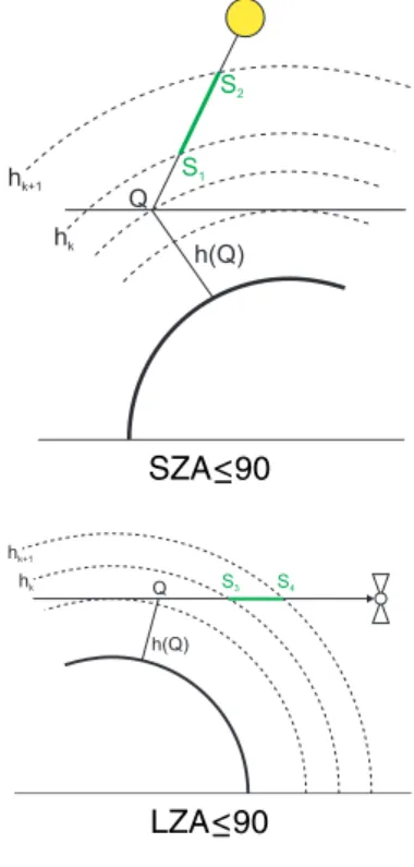
EGU For simplicity, we consider only a single species. LetN_j be the number density of the

species within the altitude layer [hj, hj+1]. To compute the derivations of the optical

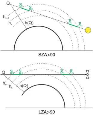
thicknesses, a number of cases have to be distinguished in terms of the solar zenith angle (SZA) and the LOS zenith angle (LZA) (see Figs.7,8):

LZA≤90 : ∂τsun(Q, λ) ∂N_j =

∂ ∂N_j exp

−

Zs2

s1

N(s)·σ(λ)d s

(41)

5

LZA>90 : ∂τsun(Q, λ) ∂N_j =

∂

∂N_j exp −

Zs₂

s₁

N(s)·σ(λ)d s−

Zs₂

s₁

N(s)·σ(λ)d s

!

SZA≤90 : ∂τsat(Q, λ) ∂Nj

= ∂ ∂Nj

exp −

Zs₄

s3

N(s)·σ(λ)d s

!

(42)

SZA>90 : ∂τsat(Q, λ) ∂N_j =

∂

∂N_j exp −

Zs₄

s₃

N(s)·σ(λ)d s−

Zs4

s3

N(s)·σ(λ)d s

!

Note that ifhj+₁< h(Q), the integrals vanish.

∂E(Q, λ) ∂N_j =

ε(λ), h_j ≤h(Q)≤h_j+1

(16)

ACPD

7, 4597–4656, 2007

Title Page

Tables Figures

◭ ◮

Back Close

Full Screen / Esc

EGU The derivative of the radiance at a certain tangent altitude is calculated using the above

formulas:

∂I(λ) ∂N_j =

∂

∂N_jF0(λ)·

Z+TOA

−TOA

τsun(s, λ)·E(s, λ)·P(s)·τsat(s, λ)d s (44)

=_F₀_(λ)_·

Z+_TOA

−TOA

"

∂ ∂Nj

τsun(s, λ)·E(s, λ)·P(s)·τsat(s, λ)

+_τ_sun_{(s, λ)}_· ∂

∂N_jE(s, λ)·P(s)·τsat(s, λ)

5

+_τ_sun_{(s, λ)}_·_E_{(s, λ)}_·_P_(s)_· ∂ ∂Nj

τsat(s, λ)

#

d s

These integrals are evaluated using quadrature algorithms as well.

3.2.3 Minimization method

The functional (39) is minimized using a Levenberg-Marquardt-style algorithm. Set

G(x)=_||F_(x)₋_y_||2 S−1

y

+_||x₋_x_a_||2 S−1

a

(45)

The gradient and the Hessian ofGare computed as follows:

∇G(x)=_KT_S−1

y (F(x)−y)+S−

1

a (x−xa) (46)

∇2G(x)=_KT_S_y−1_K +_S_a−1 ₍₄₇₎

A newton step consists of the solution of a linear system of equations:

(17)

ACPD

7, 4597–4656, 2007

Title Page

Tables Figures

◭ ◮

Back Close

Full Screen / Esc

EGU Unfortunately, the newton algorithm converges only locally and only in case the

Hes-sian is positive definite. An algorithm with global but slow convergence is the method ofgradient descent. This method uses the unit matrixI instead of the Hessian. Thus, the update step is

x→x−x∇G(x) (49)

To overcome the disadvantages of both methods, the retrieval implemented here uses the Levenberg-Marquardt method, i.e. doing step like Eq. (48) using a dynamic convex combination of the unit matrix and the Hessian instead of the Hessian alone. If the Hessian is positive definite, Eq. (48) is performed. If the Hessian fails to be positive definite, the algorithm performs

x→x+_x∆_{x , B}∆_x =_−∇G(x) ₍₅₀₎

using

B=₍₁₋_θ)∇2_G(x)+_{θI , θ}_{∈ {0.,}_0.1,_{0.2, . . . ,}_0.9,_1.} ₍₅₁₎

The parameterθis chosen minimal such thatBis positive definite. Diff_{erent stepsizes} inθare possible.

The iterations may be stopped at a pointx∗∈x ∈ Rnspecies·naltif one of the following criteria is fulfilled:

– The norm of∇G(x) falls below a certain (relative) threshold (e.g. one percent of

5

the initial norm).

– The residual||F(x)−y||is below the noise.

– The residual||F(x)−y||does not improve significantly in a certain set of successive iterations.

– The value ||x−x_a|| does not change significantly in a certain set of successive

10

(18)

ACPD

7, 4597–4656, 2007

Title Page

Tables Figures

◭ ◮

Back Close

Full Screen / Esc

EGU 3.2.4 Error analysis

The method of Optimal Estimation does not provide an exact result, but rather a proba-bility density function (PDF) of the true state of the atmosphere. This PDF is assumed to be of Gaussian shape, and the retrieval solutionxR actually constitutes the mean value. The covariance matrix can be written as follows:

S =_(KT_S_y−1_K +_S_a−1₎−1 ₍₅₂₎

The diagonal values of this matrix are the variancesσ_i2 of the state vector elements x_i∗, and hence the standard deviationsσ_i can be used as an estimation of the retrieval error. Throughout this paper, these values are used as estimations of the profile errors. Letx_t be the true state of the atmosphere. A useful information is contained in the averaging kernel matrix

A= ∂x

∗

∂xt

=_(KT_S−1

y K +S−

1

a )−1KTS−

1

y K (53)

This derivative reflects the influence of the true state on the retrieved one. An ideal

5

measurement and retrieval would result in an unity matrix A. As a real instrument like a limb sounder has a limited spatial resolution, the retrieved number density at an altitudeh(k) may be influenced by number density at lower and higher altitudes. This is quantified by the off_{-diagonal elements of the}_k_{-th row of}_{A. The vertical resolution} can thus be estimated as the full-width-half-maximum (FWHM) of the averaging kernel

10

function (which is discretely represented by thek-th row ofA) for this altitude.

Moreover, the sum of thek-th row of Acan be used as an estimation of the mea-surement response. When it is close to 1, the retrieval result is completely determined by the measurement and not by the a priori.

The measurements of Mg and Mg+ presented here exhibit very poor averaging

ker-15

(19)

ACPD

7, 4597–4656, 2007

Title Page

Tables Figures

◭ ◮

Back Close

Full Screen / Esc

EGU 3.3 Thermospheric content

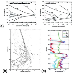
Model calculations as well as rocket soundings (Plane and Helmer,1995; Fritzenwall-ner and Kopp., 1998; McNeil et al., 1998; Roddy et al., 2004) indicate the highest number densities of metallic species at altitudes at or above the top tangent height of SCIAMACHY (92 km), see Fig.9.

5

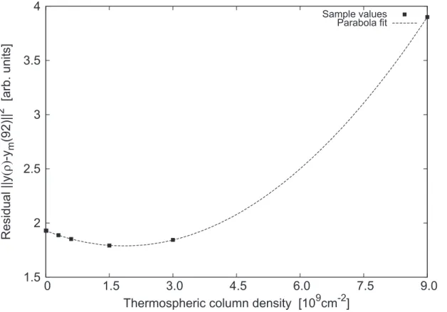
However, as a inherent feature of limb geometry, information about higher tangent altitudes is contained in every tangent altitude covered by SCIAMACHY. To gain infor-mation about the thermospheric content, the topmost limb scan is treated as a quasi-nadir measurement of the thermosphere. Self-absorption is very weak (however, it is accounted for in the retrieval) and absorption by scattering out of the LOS as well as

10

absorption by O3is negligible at these high altitudes. Thus the signal of a certain

emis-sion species at 92 km depends almost linearly on the column density of this species (see Fig.10).

The one-dimensional Newton method is used to estimate the thermospheric con-tent. Let y(ρ) be the forward computation vector corresponding to a thermospheric

15

contentρ (given e.g. in cm−2). The measurement at 92 km tangent altitude may be denotedym(92). The minimum ρT of the function F(ρ)=||y(ρ)−ym(92)||2 then gives a good estimation of the thermospheric content.

3.4 Numerical issues

Though the general approach of discretization and numerical quadrature will lead to

20

(20)

ACPD

7, 4597–4656, 2007

Title Page

Tables Figures

◭ ◮

Back Close

Full Screen / Esc

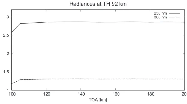
EGU 3.4.1 Choice of TOA

The forward modelled radiance at high altitudes depends on the choice of the TOA – higher values of TOA will result in higher radiances. Although this is true for arbitrarily high TOA, the change in radiances tends to zero as the TOA increases. It has been found that radiances at all wavelengths within the range considered here increase less

5

than 1% when changing the TOA from 110 to 120 km. Thus, a TOA of 120 km is chosen throughout the whole radiative transfer code.

3.4.2 Adaptive quadrature grids

The accuracy of the numerical quadrature depends crucily on the number and position of the quadrature points.

10

First, the LOS is divided in more parts if the tangent altitude decreases. The length of the LOS within the atmosphere varies from more than 1000 km at low tangent alitudes of 55–60 km to about 200 km at the topmost tangent height 92 km. This is accounted for. The lower the tangent altitude the more often the RTE is evaluated.

Second, the traverse length of a sun-bound ray increases if the SZA increases. At

15

30 SZA the way a ray has to travel is about 70% less than at 60 SZA. Changing from 60 to 80, the path length increases by a factor of more than 2. This is accounted for. The higher the SZA, the more quadrature points are chosen along a ray.

3.4.3 Separation of retrieval for diff_{erent species}

Rayleigh backscatter is a broadband eff_{ect. Line emissions, however, only feature}

ob-20

servable signals at very few isolated wavelengths. Moreover, the backscatter radiances at wavelengths diff_{erent from the emission/excitation wavelengths are not correlated} with the emissions itself. A two-step retrieval has been developed to exploit this fact.

In a first step, the air and O3 densities are determined from backscatter radiances

near the emission wavelength. It is assumed that instrumental errors such as

(21)

ACPD

7, 4597–4656, 2007

Title Page

Tables Figures

◭ ◮

Back Close

Full Screen / Esc

EGU tion behave similar for nearby wavelengths. Thus one may assume that a good

back-ground fit obtained from the first retrieval step will stay good when the wavelengths under consideration are changed a little bit for the second retrieval. The second re-trieval then treats air and O3 density as fixed while the number densities of the

emis-sion species are determined. These two steps provide a more reliable separation of

5

the background radiance from the emission than using a fixed profile of air and O3 for

the retrieval of the emission species.

3.4.4 Relative deviations instead of absolute values

The radiative impact of the various species involved in the retrieval is highly variable. For example, the number density of mesospheric ozone is roughly six orders of

mag-10

nitude smaller than the air density within the same altitude region. Though the ab-sorption cross section of O₃is larger than the Rayleigh scattering cross section of air, the absorption coeffi_{cients di}ff_{er by up to four orders of magnitude, depending on the} wavelength region.

To make computations more homogeneous and comparable, the estimated retrieval parameters (i.e. the atmospheric state vector) are not the number densities of the atmo-spheric species itself but rather their deviations from a respective given a priori profile. That is,

x=_xa+_xδ ₍₅₄₎

where the actual retrieval result is given by

xδ x =

  

x₁δ/x1

.. .

x_nspeciesδ _·_nalt/xnspecies·nalt

 

(22)

ACPD

7, 4597–4656, 2007

Title Page

Tables Figures

◭ ◮

Back Close

Full Screen / Esc

EGU The usual first order Taylor series expansion for the forward model operatorF

F(x+ ∆_x)_≈_F_(x)+_K _·∆_x _resp. ∆_y_i _≈X j

K_{i j}∆_x_j ₍₅₆₎

thus can be rewritten in the following manner:

F(x+ ∆_x)₋_F_(x) F(x) ≈Ke·

∆_x

x resp. ∆_y_i

yi

≈X j

e

K_{i j} ∆_x_j

xj

, (57)

whereKeis given by

e

Ki j =Ki j · xj yi

(58)

According to this notation, Ke_{i j} denotes the fractional variation of the radiances with respect to to the fractional variation of the atmospheric parameters.

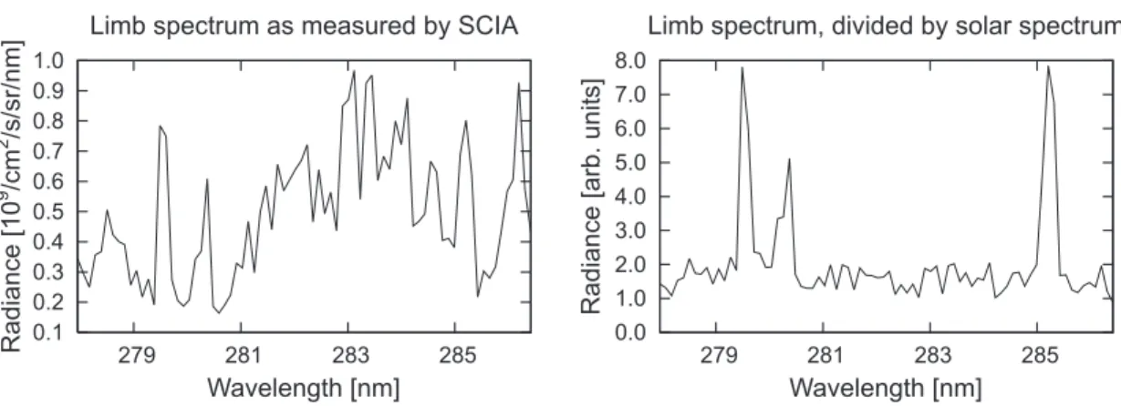
3.4.5 Improvement of S/N

The emission signals are very small and heavily contaminated by noise. To get a more distinct signal, the measured spectrum is divided through by a solar spectrum (see

5

Fig.12). To prevent artefacts that are due to the diff_{erent wavelength scales of the limb} and the sun spectrum, the wavelength grid of the latter is adjusted to the grid of the first using a shift-and-squeeze algorithm.

3.4.6 Preconditioning by onion-peeling

Though the Levenberg-Marquardt is at least in theory a globally converging algorithm, it

10

(23)

ACPD

7, 4597–4656, 2007

Title Page

Tables Figures

◭ ◮

Back Close

Full Screen / Esc

EGU may result in slow convergence or large oscillations of the number density profiles. The

latter is due to the fact that several local minima of the retrieval functional (5) (Sect. 2.3) may be located very close to each other.

This is particularly true for the retrieval of the emission species Mg and Mg+, since the signal is very weak in comparison to the measurement noise (S/N/2).

5

To obtain a preliminary estimate of the number density at each tangent height, an onion-peeling method is used as a first step. It uses similar, multiply times applied method as the thermospheric estimation (Sect. 3). After determination of the thermo-spheric content, the following steps are performed for each tangent altitudeH(k) from the top tangent height on downward. Note that for each species these steps have to

10

be performed likewise.

1. Consider the altitude interval

A_k:=

_H_(k₋₁₎₊_H_(k₎

2 ,

H(k)+_H_(k+₁₎ 2

, (59)

centered around tangent altitude H(k). Keep all number densities at higher alti-tudes fixed.

2. Assume number densities to be equal at all altitudes withinAk (assign the name ρ, say, to this value. See Fig.13a) and minimize the functional

F(ρ)=_||y_(ρ)₋_y_m_(k)||2+_γ||ρ₋_ρ₀_||2 ₍₆₀₎

Here,ym(k) denotes the measurement at tangent altitudekandy(ρ) denotes the modelled radiances that are obtained by convolution overAk, assuming all

num-15

(24)

ACPD

7, 4597–4656, 2007

Title Page

Tables Figures

◭ ◮

Back Close

Full Screen / Esc

EGU Note that in case the radiative transfer is fairly linear, the above functional is well

approximated by a parabola, any optimization method such as Newton’s method or Regula falsi (the latter is chosen here due to computational time reasons) will do well.

The number density profiles with respect to the fine altitude grid are obviously

piece-5

wise constant. Interpolation to the retrieval grid then delivers profiles that are used as new initial profiles for the conventional optimal estimation retrieval (Fig.13b).

3.5 Sensitivity analysis

A number of retrieval runs has been performed to analyse the dependency and stabil-ity of the retrieved profiles with respect to the input parameters (absorption/scattering

10

cross sections) as well as the measured data (irradiances, radiances, wavelength grid, SZA, SAA, tangent altitude grid). As a typical setup of SCIAMACHY measurements, the following parameters have been chosen to produce a synthetic measurement:

1. SZA=_{60, SAA}=₃₀

2. ACE model profiles of air density and O₃density

15

3. Measurement noise 20%

The retrieval is run with the following setup:

1. Wavelength grid: three wavelength bins of 10 pixel each, situated at 250–251 nm, 270–271 nm, 295–296 nm. Similar results have been obtained using eight wave-length bins located between 250–300 nm (see Sect.4.1).

20

2. Initial profile guess: true profile increased by 25%

(25)

ACPD

7, 4597–4656, 2007

Title Page

Tables Figures

◭ ◮

Back Close

Full Screen / Esc

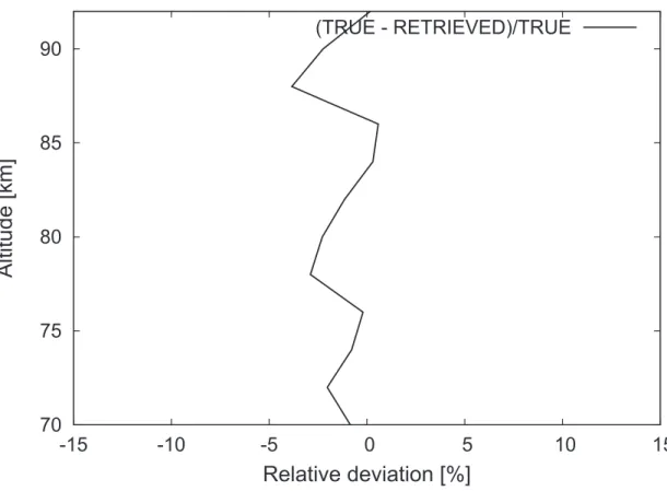
EGU At first, the retrieval was run without artificial errors on the parameters and measured

data. The true profile as reproduced by the retrieval is very good. The absolute values of the deviations are less than 4% (see Fig.14). In terms of an artificial measurement noise of 20%, this is a very good value.

It has been observed that the retrieval is error-decreasing. That is, introduction of

5

artificial errors of a certain size results in retrieval errors of smaller size. In detail, the following errors have been considered:

– An error of±10% in the solar angles (zenith and azimuth). This is approximately the standard deviation when averaging all angles (zenith and azimuth, respec-tively) over one state, i.e. one limb scan from the bottom to the top. This

er-10

ror propagates through the retrieval to end up with a profile error of 6% or less (Figs.16a, b).

– An error in the measured radiance of ±10% (Fig. 16a). This value is estimated from pre-flight design analysis (Bovensmann et al.).

– A wavelength stability of ±.003 nm has been estimated by (Bovensmann et al.,

15

1999). This error has virtually no eff_{ect on the retrieved profiles (Fig.}_16b).

– The absorption cross sections have been perturbed by ±10%. This value ac-counts well for the temperature-dependency the absorption cross section of ozone as well as for the relative errors in laboratory determination of these values (Bur-rows et al., 1999). This perturbation shows increasing eff_{ect at lower altitudes}

20

(Fig.16a). This is quite reasonable, as the absorption has a minor contribution to the limb scattered radiance at high altitudes.

– The scattering cross sections have been perturbed by±10%. This value has been chosen according to that of the absorption cross sections. Relative deviations from the true profile are altitude independent, but stay well within±10% (Fig.16a).

25

(26)

ACPD

7, 4597–4656, 2007

Title Page

Tables Figures

◭ ◮

Back Close

Full Screen / Esc

EGU be wrong by up to 1.5 km (v. Savigny et al.,2006). For completeness, a

down-shift is considered as well as an updown-shift by 1.5 km. The tangent height grid of the synthetic measurement is decreased resp. increased by 1.5 km and the retrieved profile is compared to the true profile. Surprisingly at first sight, the off_{set between} the retrieved and the true profile has the same sign but is approximately half the

5

off_{set of the respective tangent height grids. This may be due to the limited height} resolution of SCIAMACHY, which is found to be approximately 5 km (twice the value of the tangent height step), see Sect.4.1.

4 Results

4.1 Mesospheric air density

10

4.1.1 Retrieval settings

Mesospheric air density is retrieved from Rayleigh backscattered radiance.

As Rayleigh scattering is highly wavelength dependent, the retrieval is supposed to obtain information from a very large wavelength range. However, computational capacity and time limits restrict the coverable range. To overcome this disadvantages,

15

a number of microwindows consisting of a small number of detector pixels is selected. The complete set of these windows covers a large part of SCIAMACHY UV channel 1 (see Fig.19). The wavelength microwindows are chosen in a way not to contain any atmospheric emission features that would perturb the Rayleigh information.

At lower wavelengths (≤260 nm) the O3 absorption in the Hartley-Huggins bands

20

has a large impact on the radiative transfer. The ozone number density is contained as an additional retrieval species. However, very little information is contained in the mesospheric measurement. Thus no scientific benefit is gained from these results.

(27)

ACPD

7, 4597–4656, 2007

Title Page

Tables Figures

◭ ◮

Back Close

Full Screen / Esc

EGU 4.1.2 Results

The retrieved profile of air density (Fig.20) is in reasonable agreement with the model profile. The strong increase at altitudes above 85 km is due to straylight in SCIA-MACHY’s upper tangent heights (van Soest, 2006). However, the spectral data of SCIAMACHY have not been corrected for the pointing error yet. This off_{set accounts}

5

for values of up to 2 km (v. Savigny et al.,2005). That is, retrieved profiles might be shifted upwards by this value. Note that the off_{set between the model profile and the} re-trieved one is approximately 1.5 km. Note, however, there is no correlation yet between the choice of the a priori and the geolocation of the tangent point.

The averaging kernels as shown in Fig.21 exhibit a FWHM of≈5 km. This can be

10

used as an estimate of the instrument’s altitude resolution. The information content is near unity, indicating that the results are determined primarily by the measurement and not by the a priori. See Sect.3.2.4for a stringent derivation of averaging kernels.

Using support by mesospheric and thermospheric atmosphere models, possible ap-plications for the retrieval of mesospheric air density contain retrievals of temperature

15

as well as pressure. However, the retrieval results of air and O₃ are used primarily to have a good approximation of the background radiance, which is essential for the retrieval of emission species. Thus, the results in terms of air density are not discussed in further detail here.

4.2 Mesospheric Mg and Mg+

20

4.2.1 Retrieval setting

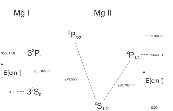
Mesospheric Mg and Mg+number densities are retrieved from emission features around 280 resp. 285 nm. These emission features are due to resonance fluorescence from the first excited states into the ground state (see Sect.3.1.4and Fig.6). Mg+ delivers two strong emission lines (279.553 nm, 280.270 nm), whereas only one strong neutral

25

(28)

ACPD

7, 4597–4656, 2007

Title Page

Tables Figures

◭ ◮

Back Close

Full Screen / Esc

EGU The measured radiances are divided through by a solar spectrum of the same day

measured by SCIAMACHY. A retrieval using the absolute radiances is possible in prin-ciple but leads to very poor results compared to those using relative radiances.

Before running the actual Optimal Estimation retrieval, a preconditiong is performed to provide good a priori knowledge. Due to this, the influence of the measurement on

5

the final retrieval result as calculated from the averaging kernels (see Sect. 3.2.4) is very weak. Note, however, that the a priori itself contains much information from the measurement.

4.2.2 Results

The Mg profile shows a pronounced peak around 85 km, see Fig.23. These values are

10

significant in terms of the retrieval/measurement error as well as in terms of the infor-mation content that can be read from the averaging kernels. This result is consistent with model calculations (Fritzenwallner and Kopp., 1998;Plane et al., 2003). These calculations suggest the maximum abundance of neutral Mg being located around 86– 89 km and the peak concentration of Mg+ located around 95–100 km (see Figs. 9a,

15

b).

The profile of the ionized species Mg+ is virtually zero below 85 km, though the limb signal is well pronounced (see Fig.25). This indicates that the major abundance of ionized Magnesium is in the thermosphere at altitudes above the top tangent altitude of SCIAMACHY. The thermospheric column densities agree well with LIDAR observations

20

of the total column done over Wallops Island (36.9 N, 1.7×1010 cm−2) and Sardinia (36.2 N, 2.1×109cm−2) (comp.Fritzenwallner and Kopp.,1998).

As can be read from the averaging kernels shown in Figs. 24 and 26, the vertical resolution of the retrieval is approximately 5 km. The information content for Mg is well around 1 for altitudes above 75 km. Mg+, however, performs worse. The measurement

25

(29)

ACPD

7, 4597–4656, 2007

Title Page

Tables Figures

◭ ◮

Back Close

Full Screen / Esc

EGU 5 Conclusions

The SCIAMACHY limb data exhibit a number of emission lines of metals species. These can be used to derive number densities on a global scale within the altitude range 65–92 km. Beside this, Rayleigh backscatter radiation can be utilized to derive mesospheric air number densities.

5

A forward model for radiative transfer calculations in the mesosphere has been devel-oped. It has been coupled to an augmented Optimal Estimation Retrieval. Numerical improvements and stabilizations (such as preconditioning) have been applied

A joint retrieval of Mg, Mg+ and mesospheric air density is now available and has been tested. The retrieval has been optimized to the corresponding species by

adap-10

tive choice of spectral microwindows. The altitude resolution (5 km) at mesospheric altitudes is found to be worse than what can be expected from the actual limb tangent altitude step and FOV width (both approx. 3 km). The pointing error of SCIAMACHY is not corrected for yet.

Retrieval results of Mg, Mg+and air density show reasonable agreement with

corre-15

sponding models. Column densities of the metallic species are in well agreement with previous rocket measurements.

Acknowledgements. Eff_{ort partly sponsored by the Air Force O}ffi_{ce of Scientific Research, Air} Force Material Command, USAF, under grant number FA8655-03-1-3035. The U.S. Govern-ment is authorized to reproduce and distribute reprints for GovernGovern-ment purpose notwithstand-20

ing any copyright notation thereon.

The views and conclusions contained herein are those of the author and should not be inter-preted as necessarily representing the official policies or endorsements, either expressed or implied, of the Air Force Office of Scientific Research or the U.S. Government.

Parts of this publication were sponsored by the University of Bremen, FNK project 01/802/03 25

(30)

ACPD

7, 4597–4656, 2007

Title Page

Tables Figures

◭ ◮

Back Close

Full Screen / Esc

EGU References

Anderson, J. G. and Barth, C. A.: Rocket Investigation of the MgI and MgII Dayglow, J.

Geo-phys. Res., 76, 3723–3731, 1971. 4605

Bovensmann, H., Burrows, J. P., Buchwitz, M., Frerick, J., Noel, S., and Rozanov, V. V.: SCIA-MACHY: Mission Objectives and Measurement Modes, J. Atmos. Sci., 56, 127–150, 1999. 5

4621

Burrows, J. P., Dehn, A., Deters, B. S. H., Richter, A., Voigt, S., and Orphal, J.: Atmo-spheric Remote–Sensing Reference Data from GOME: 2. Temperature-Dependent Absorp-tion Cross SecAbsorp-tions of O3 in the 231–794 nm range, J. Quant. Spectros. Radiat. Trans., 61, 509–517, 1999. 4604,4621

10

Chandrasekhar, S.: Radiative Transfer, Dover Publications Inc., New York, 1960.4603

Edlen, B.: The refractive index of air, Meteorologica, 2, 71–80, 1966.4604

Eichmann, K.-U.: Optimierung und Validierung des pseudosphysischen Strahlungstransport-modells GOMETRAN, Master’s thesis, University of Bremen, Institute of Environmental Physics, 1995.4604

15

Fritzenwallner, J. and Kopp., E.: Model Calculations of the Silicon and Magnesium Chemistry

in the Mesosphere and Lower Thermosphere, Adv. Space Res., 21, 859–862, 1998. 4615,

4624,4637,4655

Grebowsky, J. M., Pesnell, W. D., and Goldberg, R. A.: Do meteor showers significantly pertub the ionosphere?, J. Atmos. Solar-Terr. Phys., 60(6), 607–615, 1998. 4637

20

Hedin, A.: Extension of the MSIS Thermosphere Model into the Middle and Lower Atmosphere, J. Geophys. Res., 96, 1159–1172, 1991. 4622

Kaiser, J.: Atmospheric Parameter Retrieval from UV–Visible–NIR Limb Scattering Measure-ments, Ph.D. thesis, University of Bremen, Institute of Environmental Physics, 2001. 4603

McNeil, W. J., Shu, T. L., and Murad, E.: Differential ablation of cosmic dust and implications 25

for the relative abundances of atmospheric metals, J. Geophys. Res., 103, 10 899–10 911, 1998. 4615,4637

NIST: National Institute of Standards and Technology: Atomic Spectra Database,http://physics.

nist.gov/PhysRefData/ASD/lines form.html, 2005.4605

Noel, S., Bovensmann, H., Burrows, J. P., Frerick, J., Chance, K. V., and Goede, A. H. P.: Global 30

Atmospheric Monitoring with SCIAMACHY, Phys. Chem. Earth(C), 24, 427–434, 1999.4601

(31)

ACPD

7, 4597–4656, 2007

Title Page

Tables Figures

◭ ◮

Back Close

Full Screen / Esc

EGU

4984, 2003. 4599,4628

Plane, J. M. C. and Helmer, M.: Laboratory Study of the Reactions Mg+O₃ and MgO+O₃, Implications for the Chemistry of Magnesium in the Upper Atmosphere, Faraday Discussions, 100, 411–430, 1995. 4600,4615,4629,4630

Plane, J. M. C., Self, D. E., Vondrak, T., and Woodcock, K. R. I.: Laboratory studies and 5

modelling of mesospheric iron chemistry, Adv. Space Res., 32, 699–708, 2003. 4624

Roddy, P. A., Earle, G. D., Swenson, C. M., Carlson, C. G., and Bullett, T. W.: Relative con-centrations of molecular and metallic ions in midlatitude intermediate and sporadic E–layers, Geophys. Res. Lett., 31, L19807, doi:10.1029/2004GL020604, 2004.4615,4637

Rodgers, C. D.: Retrieval of atmospheric temperature and composition fom remote measure-10

ments of thermal radiation, Rev. Geophys. Space Phys., 14, 609–624, 1976. 4610

Rozanov, A.: Modeling of radiative transfer through a spherical planetary atmosphere, Ph.D. thesis, University of Bremen, Institute of Environmental Physics, 2001.4604

v. Savigny, C., Kaiser, J. W., Bovensmann, H., Burrows, J. P., McDermid, I. S., and Leblanc, T.: Spatial and temporal characterization of SCIAMACHY limb pointing errors during the first 15

three years of the mission, Atmos. Chem. Phys., 5, 2593–2602, 2005,

http://www.atmos-chem-phys.net/5/2593/2005/. 4623

v. Savigny, C., Bramstedt, B., Noel, S., Sinnhuber, M., and Taha, G.: Comparison of SCIA-MACHY pointing retrievals in limb and Occultation geometry, Tech. Rep. TN–IUP/IFE–2006– cvs–03, University of Bremen, Intitute of Environmental Physics, 2006.4622

20

van Soest, G.: Investigation of SCIAMACHY limb spatial straylight, Tech. Rep. SRON–EOS–

(32)

ACPD

7, 4597–4656, 2007

Title Page

Tables Figures

◭ ◮

Back Close

Full Screen / Esc

EGU

Table 1.Features of meteoric metals. S: Species, EP: Evaporation point, MA: Maximal ablation, ARM: Average relative mass. Abridged from (Plane,2003).

S EP MA ARM

Mg 1363 K 80–90 km 12.5 %

Fe 3023 K ? 11.5 %

Na 1156 K 90–110 km 0.6 %

(33)

ACPD

7, 4597–4656, 2007

Title Page

Tables Figures

◭ ◮

Back Close

Full Screen / Esc

EGU

(34)

ACPD

7, 4597–4656, 2007

Title Page

Tables Figures

◭ ◮

Back Close

Full Screen / Esc

EGU

Fig. 2. Overview of the chemistry of Mg, Mg+ and respective compounds in the upper

(35)

ACPD

7, 4597–4656, 2007

Title Page

Tables Figures

◭ ◮

Back Close

Full Screen / Esc

EGU

(36)

ACPD

7, 4597–4656, 2007

Title Page

Tables Figures

◭ ◮

Back Close

Full Screen / Esc

EGU

NO -bands

g

Fe+

Mg+

MgSi/Na /Fe

+ +

Fe/Fe+

Fe Fe /Li+ +

Na+ _O/Mg+

20040715 mean radiances

Wavelength [nm]

Radiance/Irradiance[arb.unit

s]

0 1

240 250 260 270 280 290 300

(37)

ACPD

7, 4597–4656, 2007

Title Page

Tables Figures

◭ ◮

Back Close

Full Screen / Esc

EGU

h

Earth

F ( )

0

l

I(h, )

l

LOS

TO_A

Tangent point

H

Fig. 5. The limb observational geometry of SCIAMACHY. This forward model covers tangent

(38)

ACPD

7, 4597–4656, 2007

Title Page

Tables Figures

◭ ◮

Back Close

Full Screen / Esc

EGU 2

P

_3/2

2

P

_1/2

2

S

_1/2

279.553 nm

280.702 nm

E[cm ]

-1

E[cm ]

-1

0.00 35669.31

3 S

3 ₀

3 P

3 ₁

285.165 nm 35051.36

0.00

Mg I

Mg II

35760.88

(39)

ACPD

7, 4597–4656, 2007

Title Page

Tables Figures

◭ ◮

Back Close

Full Screen / Esc

EGU hk

hk+1 Q

h(Q)

S1

S2

SZA≤90

hk

hk+1

Q

h(Q) S3 S4

LZA≤90

(40)

ACPD

7, 4597–4656, 2007

Title Page

Tables Figures

◭ ◮

Back Close

Full Screen / Esc

EGU

hk

hk+1

Q

h(Q) _S

2 S1 S1

S2

SZA>90

hk

hk+1

Q

h(Q)

S3

S3 S4 S4

LZA>90