Modelling runoff from a Himalayan debris-covered glacier

(1)

HESSD

11, 2441–2482, 2014

Modelling runofffrom a Himalayan debris-covered

glacier

K. Fujita and A. Sakai

Title Page

Abstract Introduction

Conclusions References

Tables Figures

◭ ◮

Back Close

Full Screen / Esc

Printer-friendly Version

Interactive Discussion

Discussion

P

a

per

|

D

iscussion

P

a

per

|

Discussion

P

a

per

|

Discuss

ion

P

a

per

|

Hydrol. Earth Syst. Sci. Discuss., 11, 2441–2482, 2014 www.hydrol-earth-syst-sci-discuss.net/11/2441/2014/ doi:10.5194/hessd-11-2441-2014

Hydrology and Earth System

Sciences

Open Access

Discussions

This discussion paper is/has been under review for the journal Hydrology and Earth System Sciences (HESS). Please refer to the corresponding final paper in HESS if available.

Modelling runo

_ff

from a Himalayan

debris-covered glacier

K. Fujita and A. Sakai

Graduate School of Environmental Studies, Nagoya University, Nagoya, Japan

Received: 16 January 2014 – Accepted: 10 February 2014 – Published: 26 February 2014

Correspondence to: K. Fujita ([email protected])

(2)

HESSD

11, 2441–2482, 2014

glacier

Title Page

Tables Figures

◭ ◮

Back Close

Full Screen / Esc

Discussion

P

a

per

|

D

iscussion

P

a

per

|

Discussion

P

a

per

|

Discuss

ion

P

a

per

|

Abstract

Although the processes by which glacial debris-mantles alter the melting of glacier

ice have been well studied, the mass balance and runoff patterns of Himalayan

debris-covered glaciers and the response of these factors to climate change are not well understood. Many previous studies have addressed mechanisms of ice 5

melt under debris mantles by applying multiplicative parameters derived from field experiments, and other studies have calculated the details of heat conduction through the debris layer. However, those approaches cannot be applied at catchment scales

because debris distributions are heterogeneous and difficult to measure. Here, we

establish a runoff model for a Himalayan debris-covered glacier in which the spatial

10

distribution of the thermal properties of the debris mantle is estimated from remotely sensed multi-temporal data. We validated the model for the Tsho Rolpa Glacial Lake– Trambau Glacier basin in the Nepal Himalaya, using hydro-meteorological observations obtained for a 3.5 yr period (1993–1996). We calculated long-term averages of

runoffcomponents for the period 1980–2007 using gridded reanalysis datasets. Our

15

calculations suggest that excess meltwater from the debris-covered area contributes

significantly to the total runoff, mainly because of its location at lower elevations.

Uncertainties in runoffvalues due to estimations of the thermal properties and albedo

of the debris-covered surface were assessed to be approximately 8 % of the runoff

from the debris-covered area. We evaluated the sensitivities of runoffcomponents to

20

changes in air temperature and precipitation. As expected, warmer air temperatures

increase the total runoffby increasing the melting rate; however, increased precipitation

slightly reduces the total runoff, as ice melting is suppressed by the increased snow

cover and associated high albedo. The response of total runoffto changing precipitation

is complex because of the different responses of individual components (glacier, debris,

25

(3)

HESSD

11, 2441–2482, 2014

glacier

Title Page

Tables Figures

◭ ◮

Back Close

Full Screen / Esc

Discussion

P

a

per

|

D

iscussion

P

a

per

|

Discussion

P

a

per

|

Discuss

ion

P

a

per

|

1 Introduction

Glaciers are considered to play an important role in the delivery of water resources to densely populated Asian regions (e.g. Cruz et al., 2007). Recent studies have revealed that the response of glaciers to climate variations varies considerably in Asian highland regions (e.g. Fujita and Nuimura, 2011; Bolch et al., 2012; Yao et al., 5

2012), and that the response depends in part on the characteristics of the debris mantles on Himalayan glaciers. Terminus positions of heavily debris-covered glaciers seem to be insensitive to changes in climate (Scherler et al., 2011), while surface lowering over debris-covered areas seems to be comparable to that in debris-free ablation areas (Nuimura et al., 2011, 2012; Kääb et al., 2012). It is still unclear whether 10

heterogeneity in climatic forcing or debris cover patterns is responsible for observed

temporal variations in glacial melt observed in different Himalayan glacier systems.

Experimental studies have revealed that thin debris layers accelerate the melting of underlying ice, whereas thick debris layers suppress melting (e.g. Østrem, 1959; Mattson et al., 1993). Some numerical simulations of conductive heat flux through the 15

debris layer have successfully reproduced patterns of ice melting under the debris layer (e.g. Nicholson and Benn, 2006; Reid and Brock, 2010). However, these heat conduction models cannot be applied to basin-scale mass balance calculations in debris-covered glacier systems because the spatial distributions in debris thickness and thermal conductivity are nearly impossible to measure. On the other hand, some 20

hydrological studies in glacierized catchments containing debris-covered glaciers have parameterized ice melting under the debris layer (e.g. Lambrecht et al., 2011; Anderson and Mackintosh, 2012; Immerzeel et al., 2012). Although these studies have been validated by hydrologic and/or other observational data, continuity in surface conditions over time cannot be guaranteed, especially in systems with rapidly changing glaciers. 25

In addition, the debris-covered surfaces of real glaciers exhibit highly heterogeneous and rugged topography, over which no representative thickness is obtainable. Heat

(4)

HESSD

11, 2441–2482, 2014

glacier

Title Page

Tables Figures

◭ ◮

Back Close

Full Screen / Esc

Discussion

P

a

per

|

D

iscussion

P

a

per

|

Discussion

P

a

per

|

Discuss

ion

P

a

per

|

is considered to be one of the significant sources of heat for melting in debris-covered areas (Sakai et al., 2000a, 2002). Therefore, prediction of basin-scale patterns of ice melt on debris-covered glaciers from a simple relationship between debris thickness and ice melting is exceedingly difficult.

To overcome the difficulties discussed above, we have adopted the “thermal

5

resistance” parameter proposed by Nakawo and Young (1982). This parameter is defined as the debris thickness divided by the thermal conductivity of the debris layer and its spatial variations may be obtained from remotely sensed data, such as data obtained from Landsat or ASTER imagery. Nakawo and Rana (1999) used this approach to estimate the distribution of thermal resistance on glaciers 10

from Landsat TM data, and successfully reproduced runo_ff from the debris-covered

Lirung Glacier in the Langtang region of Nepal. Subsequently, Suzuki et al. (2007) demonstrated temporally consistent values of thermal resistance on glaciers in the

Bhutan Himalaya, as determined from ASTER data taken on di_fferent dates, for

which surface temperature and albedo were calibrated using field measurements 15

conducted at the same time as ASTER acquisitions. Zhang et al. (2011, 2012) obtained the thermal resistance distribution of a debris-covered glacier in southeastern

Tibet and validated the calculated thermal resistance, melt, and runoff with in situ

measurements. However, these studies did not evaluate uncertainties in thermal

resistance values, or how these a_ffect both the calculated ice melt under the debris and

20

the resulting runoff. In this study, therefore, our goal was to obtain thermal resistance

values and to evaluate uncertainties in the values based on ASTER data acquired

in di_fferent seasons and years. In addition, we establish an integrated runo_ff model

that incorporates variations in surface conditions, such as covered and debris-free glacier surfaces as well as ice-debris-free terrain. Model performance was tested for 25

(5)

HESSD

11, 2441–2482, 2014

glacier

Title Page

Tables Figures

◭ ◮

Back Close

Full Screen / Esc

Discussion

P

a

per

|

D

iscussion

P

a

per

|

Discussion

P

a

per

|

Discuss

ion

P

a

per

|

2 Location, data and models

2.1 Delineation and classification of the catchment

We chose as our study site the Tsho Rolpa Glacial Lake–Trambau Glacier basin

located at the head of the Rolwaring Valley, in the east Nepal Himalaya (27.9◦N,

86.5◦E, Fig. 1). Tsho Rolpa (the word “Tsho” means “lake” in the local language) is

5

one of the largest glacial lakes in the Nepal Himalaya. We delineated the basin using a digital elevation model produced from multi-temporal ASTER data (ASTER-GDEM, 2009; Tachikawa et al., 2011). The basin extends from 4500 to 6850 m a.s.l., with a total

area of 76.5 km2(Fig. 1a and Table 1).

We divided the surface features of the basin into four categories: debris-covered 10

glacier (debris), debris-free glacier (glacier), ice-free terrain (ground), and lake surface

(Tsho Rolpa) to perform the following runoffcalculations. Using the clearest available

ASTER image acquired on February 2006 (Fig. 1a), we calculated the normalized

difference water index (NW) and normalized difference snow/ice index (NS) from the

following equations: 15

NW=(r3−r1)/(r3+r1) (1)

NS=(r2−r4)/(r2+r4) (2)

Here r denotes reflectance of each band (subscript number) in the ASTER sensors.

The NW has been successfully used to delineate glacial lake boundaries in the

20

Himalayas (Fujita et al., 2009). TheN_S has been used to evaluate snow cover extent

in North America (Hulka, 2008). Thresholds of NW and NS are assumed to be 0.42

and 0.94, respectively, to best distinguish the surfaces. Debris-covered surface was visually distinguished from ice-free terrain using surface morphology such as rugged

relief and ice flow features (Nagai et al., 2013). Steep slope terrain (steeper than 30◦)

25

(6)

HESSD

11, 2441–2482, 2014

glacier

Title Page

Tables Figures

◭ ◮

Back Close

Full Screen / Esc

Discussion

P

a

per

|

D

iscussion

P

a

per

|

Discussion

P

a

per

|

Discuss

ion

P

a

per

|

2.2 Thermal resistance

Thermal resistance is defined as debris thickness divided by the thermal conductivity of the debris layer (Nakawo and Young, 1982). Suzuki et al. (2007) established a methodology to obtain the thermal resistance distribution from ASTER and reanalysis climate data. Zhang et al. (2011) confirmed that the distribution of thermal resistance 5

was well correlated with that of debris thickness from in situ measurements over a southeastern Tibetan glacier with a rather gentle and homogeneous debris-covered surface. We obtained the thermal resistance of the debris-covered area from

multi-temporal ASTER data following their methods. The thermal resistance (RT, m

2

K W−1) is defined as:

10

RT=h/λ, (3)

wherehis debris thickness (m) andλis thermal conductivity (W m−1K−1) of the debris

layer. Assuming no heat storage in the debris layer, no heat conduction into temperate glacier ice, and a linear temperature profile within the debris layer, the conductive heat 15

flux through the debris layer (Gd, W m

−2

) is described as:

Gd=(Ts−Ti)/RT, (4)

where Ts is the surface temperature (

◦

C) and Ti the temperature at the interface

between debris and ice, which is assumed to be melting point (0◦C). The conductive

20

heat flux from the surface toward the debris–ice interface is described as a residual term of the heat balance at the debris surface, according to:

Gd=Ts/RT=(1−αd)RS+RL−εσ(Ts+273.15)4+HS+HL, (5)

whereRSandRLare the downward short-wave and long-wave radiation fluxes (W m

−2 ), 25

respectively, HS and HL are the sensible and latent turbulent heat fluxes (W m

−2 ),

(7)

HESSD

11, 2441–2482, 2014

glacier

Title Page

Tables Figures

◭ ◮

Back Close

Full Screen / Esc

Discussion

P

a

per

|

D

iscussion

P

a

per

|

Discussion

P

a

per

|

Discuss

ion

P

a

per

|

upward long-wave radiation (W m−2) according to the Stefan–Boltzmann equation with

a constant ofσ (5.67×10−8W m−2K−4) and surface temperature (T_s), with emissivity

(ε, dimensionless) assumed to be 1. All components except for Gd are positive when

the fluxes are directed towards the debris surface. Although turbulent heat fluxes have to be taken into account in the exact heat exchange over the debris surface, Suzuki 5

et al. (2007) demonstrated that these fluxes are negligible at Himalayan high elevation because the density of air, the material transferring these fluxes, is approximately half that at sea level. Clear sky conditions, which are required for satellite data utilization, are also associated with a reduced importance of turbulent heat fluxes, especially of

latent heat. We therefore assumed that the turbulent heat fluxes were zero (HS=HL=

10

0). We can then obtain the thermal resistance at a given point without knowing the debris thickness and thermal conductivity if we know the downward short-wave and long-wave radiation fluxes, the albedo, and the surface temperature. We selected eight cloud-free images of ASTER level 3A1 data, which is a semi-standard ortho-rectified product available from ERSDAC Japan (Table S1). Surface albedo is calculated using 15

three visible near infrared sensors (VNIR; bands 1–3) using the equations described in Yüksel et al. (2008). Surface temperature is obtained from an average of five sensors in the thermal infrared (TIR; bands 10–14) using the formula proposed by Alley and Nilsen (2001). The spatial resolution of the thermal resistance is then constrained by the coarsest resolution of the ASTER TIR sensors (90 m). We utilize NCEP/NCAR 20

reanalysis 6 hourly data (Kalnay et al., 1996) for both downward radiation fluxes at the time (noon) closest to ASTER acquisition.

2.3 Models

2.3.1 Energy and mass balance of debris-covered surface

We calculate heat balance at the debris-covered surface using Eq. (5), but also 25

(8)

HESSD

11, 2441–2482, 2014

glacier

Title Page

Tables Figures

◭ ◮

Back Close

Full Screen / Esc

Discussion

P

a

per

|

D

iscussion

P

a

per

|

Discussion

P

a

per

|

Discuss

ion

P

a

per

|

neglected when the thermal resistance was obtained under the clear sky assumption; see Sect. 2.2). The turbulent fluxes are estimated by bulk formulae as:

HS=cpρaCdU(Ta−Ts), (6)

H_L=l_eρ_aC_dUτ_w[h_rq(T_a)−q(T_s)], (7)

τw=e

−300R_T

, (8)

5

wherecpis the specific heat of air (1006 J K

−1

kg−1),ρa is air density (kg m

−3

), which depends on elevation,Cdis the bulk coefficient for the debris surface (0.005),U is wind speed (m s−1),Ta is air temperature (

◦

C),le is the latent heat of evaporation of water

(2.5×106J kg−1),hris relative humidity (dimensionless),qis saturated specific humidity 10

(kg kg−1), andτwis wetness parameter (dimensionless). Suzuki et al. (2007) revealed

that the debris surface was wet (τw≈1) when its thickness was thin and became

exponentially drier (τw≈0) with increased thermal resistance in the Bhutan Himalaya.

Air temperature, solar radiation, relative humidity, and wind speed are required as

input variables. Downward long-wave radiation (W m−2) is estimated from an empirical

15

equation using air temperature, relative humidity and the ratio of solar radiation to that at the top of atmosphere based on Glover and McCulloch (1958) and Kondo (1994). We determine the surface temperature that satisfies Eq. (5) by iterative calculation. Once the surface temperature is determined and the heat flux toward the ice–debris

interface is positive, the daily melt of ice beneath the debris layer (Md, kg m

−2 day−1 20

or mm water equivalent (w.e.) day−1) and then daily runoffwater (Dd, mm w.e. day

−1 ) generated at a given point are obtained as:

Md=tdayGd/lm, (9)

Dd=Md+Pr+max[HL/le, 0], (10)

25

where tday is the length of a day (86 400 s), lm is the latent heat of fusion of ice

(9)

HESSD

11, 2441–2482, 2014

glacier

Title Page

Tables Figures

◭ ◮

Back Close

Full Screen / Esc

Discussion

P

a

per

|

D

iscussion

P

a

per

|

Discussion

P

a

per

|

Discuss

ion

P

a

per

|

obtained from daily precipitation and air temperature as described later. It is assumed that all heat flux into the debris layer is used to melt ice. Condensation of vapour is also taken into account if available (HL/le) though it is generally negligible in many cases. Although the albedo of the debris surface is obtained from the ASTER data, seasonal snow may occasionally cover the debris surface. If snow covers the debris surface, the 5

heat balance and daily snow melt are estimated as:

max[Qs, 0]=(1−αs)RS+RL−εσ(Ts+273.15)4+HS+HL, (11)

Ms=tdayQs/lm, (12)

whereα_s is the surface albedo of snow (dimensionless), Q_s is the surface heat flux

10

(W m−2) andMsis the daily snow melt (mm w.e. day

−1

). There is assumed to be no ice

melt beneath the debris layer until the snow cover completely melts away. Daily runoff

in the presence of snow is thus obtained from Eq. (10), but with the ice melt beneath

the debris-layer (Md) replaced by the snow-melt (Ms). The temporal change in snow

albedo is calculated as described in Sect. 2.3.4 below. The spatial resolution for the 15

debris-covered surface is 90 m, which is constrained by the ASTER TIR data used to obtain the surface temperature in the thermal resistance calculation (Sect. 2.2).

2.3.2 Energy and mass balance of the debris-free glacier

Energy and mass balance over the debris-free glacier surface are calculated in 50 m elevation bands from a model established by Fujita and Ageta (2000), which has 20

successfully calculated the glacier mass balance, equilibrium line altitude and runoff

of several Asian glaciers (e.g. Fujita et al., 2007, 2011; Sakai et al., 2009a, 2010; Fujita and Nuimura, 2011; Zhang et al., 2013). The basic equation can be written:

max[Q_g, 0]=(1−α_s)R_S+R_L−εσ(T_s+273.15)4+H_S+H_L+G_g, (13)

25

whereQg is the heat flux for ice/snow melting (W m

−2

) andGg is the conductive heat

(10)

HESSD

11, 2441–2482, 2014

glacier

Title Page

Tables Figures

◭ ◮

Back Close

Full Screen / Esc

Discussion

P

a

per

|

D

iscussion

P

a

per

|

Discussion

P

a

per

|

Discuss

ion

P

a

per

|

towards the glacier surface. Turbulent heat fluxes are calculated using the same bulk

method given in Eqs. (6) and (7), but using an alternative bulk coefficient for the snow–

ice surface (Cs, 0.002, dimensionless) and a constant wetness parameter (τw=1). We

determine the surface temperature by iterative calculations, in which the conductive heat flux into the glacier ice is calculated by changing the ice temperature profile. Daily 5

runoffwater (Dg, mm w.e. day

−1

) is obtained as:

Dg=tdayQg/lm+Pr+max[HL/le, 0]−Rf, (14)

whereRf is refrozen ice in the snow layer (mm w.e. day

−1

), which is obtained from the change in the ice temperature profile when surface water is present. All details are 10

described in Fujita and Ageta (2000) and Fujita et al. (2007).

2.3.3 Runofffrom ice-free terrain and the lake

Runofffrom ice-free terrain is calculated for 50 m elevation bands, based on a simple

bucket model proposed by Motoya and Kondo (1999). The potential evaporation rate (Ep, mm w.e. day

−1

) is obtained from the energy balance: 15

(1−α_w)RS+RL−εσ(Ts+273.15)4+HS+HL=0, (15)

βEp=−tdayHL/le=−tdayρaβCt(U)[hrq(Ta)−q(Ts)], (16)

where α_w is the albedo of ice-free terrain (dimensionless), which is assumed to be

0.1, β is the evaporation efficiency (dimensionless), which depends on soil moisture

20

content:

β=Wa/Wamax, (17)

whereWaandWamax are the water content and the maximum water content of surface

storage just below the surface, respectively (Fig. S1). Both are expressed in terms of 25

(11)

HESSD

11, 2441–2482, 2014

glacier

Title Page

Tables Figures

◭ ◮

Back Close

Full Screen / Esc

Discussion

P

a

per

|

D

iscussion

P

a

per

|

Discussion

P

a

per

|

Discuss

ion

P

a

per

|

to be 5.0 mm w.e. The bulk coefficient (Ct, dimensionless) is parameterized with wind

speed (U, m s−1) as:

Ct(U)=0.0027+0.0031U. (18)

Runoff from the ice-free terrain (Dt, mm w.e. day

−1

) is obtained when the surface 5

storage is full:

max[Dt, 0]=Pr+max[Ms+max[HL/le, 0], 0]−βEp−(Wamax−Wa), (19)

Wn=Wamax, (20)

whereWnis the water content of the first bucket (mm w.e.) in the next time step (next

10

day). If there is snow cover, snow-melt (Ms) is calculated using Eqs. (11) and (12), in

which direct liquid condensation is taken into account if available. If there is no snow,

evaporated water (βEp) is reduced from the rainwater value. Water is first used to fill

the surface storage capacity (Wamax−Wa) in all cases. If there is insufficient water to fill

the surface storage, no runoffis generated (D_t=0) and the water content in the next

15

time step is given by:

Wn=max[Pr−βEp+Wa, 0]. (21)

If evaporation is greater than the sum of rain and water content, evaporated water

is constrained by the water in the surface storage (βEp=Wa) and no water content is

20

expected in the next time step (Wn=0).

We have little information on the water balance of the Tsho Rolpa Glacial Lake, although the water circulation within the lake has been thoroughly investigated (Sakai et al., 2000b). Therefore we assumed that precipitation would immediately be removed

as runoff from the lake (Dl, mm w.e. day

−1

), giving the maximum runoff without

25

(12)

HESSD

11, 2441–2482, 2014

glacier

Title Page

Tables Figures

◭ ◮

Back Close

Full Screen / Esc

Discussion

P

a

per

|

D

iscussion

P

a

per

|

Discussion

P

a

per

|

Discuss

ion

P

a

per

|

2.3.4 Snow albedo

Snow surface albedo on a given day (dimensionless) is calculated with a scheme proposed by Kondo and Xu (1997), in which an exponential reduction of snow albedo with time after a fresh snowfall is assumed:

αday=(αday−1−αf)e

−1/k

+αf, (22)

5

where day is the number of days after the latest fresh snow date, which is set to zero

(day=0) when snowfall is greater than 5 mm w.e., andαf, the albedo of firn, is taken

as the minimum snow albedo (0.4, dimensionless). The parameter k depends on air

temperature, according to: 10

k=5.5−3.0T_a [T_a<0.5◦C],

k=4.0 [Ta≥0.5

◦

C]. (23)

The albedo of the initial fresh snow (day=0) also depends on air temperature:

α0=0.88 [Ta<−1.0

◦

C], 15

α0=0.76−0.12Ta [−1.0

◦

C≤T_a≤3.0◦

C],

α0=0.40 [Ta>3.0

◦

C]. (24)

Surface albedo is affected by the glacier ice or debris surface if the snow layer is thin. According to Giddings and LaChapelle (1961), the penetration of solar radiation into 20

snow is assumed to follow Fick’s second law of diffusion with a term for simultaneous

absorption, and the surface snow albedo (αs, dimensionless) over the underlying ice

or debris surface is calculated as:

αs=[2−w(1−y)]/[2+w(1−y)],

w=2(1−α_day)/(1₊α_day), 25

(13)

HESSD

11, 2441–2482, 2014

glacier

Title Page

Tables Figures

◭ ◮

Back Close

Full Screen / Esc

Discussion

P

a

per

|

D

iscussion

P

a

per

|

Discussion

P

a

per

|

Discuss

ion

P

a

per

|

whereK is the extinction coefficient of snow (30 m−1; Greuell and Konzelmann, 1994),

x is the depth of the snow layer (m), and αb is the albedo of the underlying surface

(dimensionless), which is taken to be ice (αi) or debris (αd) based on the targets. The

albedo of glacier ice (αi) is assumed to be 0.2 based on our field observations on Asian

glaciers (Takeuchi and Li, 2008; Fujita et al., 2011). 5

2.3.5 Bucket model calculating river runo_ff

All water generated over the debris-covered part (Dd), debris-free snow or ice (Dg),

ice-free terrain (Dt) and the lake (Dl) is added to the river system through two types of storage, internal and ground storages (Motoya and Kondo, 1999). A schematic diagram that also includes the surface storage for ice-free terrain is shown in Fig. S1. The 10

surface water inflows (Dd,Dg,Dt,Dl) are added to the internal storage. Outflow from

the internal storage (Fb, mm w.e. day

−1

) will occur and be directly added to the final

runo_ffwhen the volume of water stored (Wb, mm w.e.) exceeds the maximum capacity

(Wbmax, 500 mm w.e.) according to:

Fb=Fa−(Wbmax−Wb) (26) 15

where Fa is the total inflow into the internal storage, which is made up of the

individual surface water inflows (Dd, Dg, Dt, Dl). Leakage from the internal storage (Fc, mm w.e. day

−1

) is simultaneously calculated as:

Fc=kbWb, (27)

20

wherekb is a leak rate parameter assumed to be 0.3 (dimensionless). It implies that

30 % of the internally stored water will be lost in a day. Part of the leakage from the

internal storage will be directly added to the final runoffand the rest will flow into the

ground storage (W_c, mm w.e.). There is no limit on the capacity of the ground storage.

25

Leakage from the ground storage (Fd, mm w.e. day

−1

) is given by:

(14)

HESSD

11, 2441–2482, 2014

glacier

Title Page

Tables Figures

◭ ◮

Back Close

Full Screen / Esc

Discussion

P

a

per

|

D

iscussion

P

a

per

|

Discussion

P

a

per

|

Discuss

ion

P

a

per

|

where kc is a leak rate parameter assumed to be 0.03 (dimensionless). This flow

will form the continuous basal flow of the river system. We obtain the final runoff (Ff,

mm w.e. day−1) as:

Ff=Fb+rcFc+Fd. (29) 5

The fraction (rc, dimensionless) is assumed to be 0.8. The final runoff can be

calculated for individual runoffs from the debris-covered surface (Rd), the debris-free

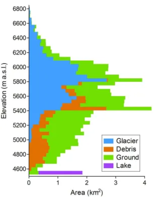
glacier (Rg), the ice-free terrain (Rt), and the lake (Rl). We summarize these runoffs by considering a debris grid with 90 m resolution and the hypsometry of the debris-free glacier surface and ice-free terrain in 50 m elevation bands (Fig. 2).

10

2.3.6 Probability of snow and rain

Precipitation across the Himalayan regions takes place mainly during the summer monsoon season so that the precipitation phase (snowfall or rainfall) has to be taken into account. Based on observational reports in Tibet (Ueno et al., 1994; Sakai et al., 2006a), we assume the probability of snowfall (Ps, mm w.e.) and rainfall (Pr, mm w.e.) to 15

depend on air temperature as follows:

Ps=Pp [Ta≤0.0

◦

C],

Ps=(1−Ta/4.0)Pp [0.0

◦

C< Ta<4.0

◦

C],

Ps=0 [Ta≥4.0

◦

C], (30)

Pr=Pp−Ps (31)

20

wherePpis daily precipitation (mm w.e.).

2.4 Meteorological and hydrological data

(15)

HESSD

11, 2441–2482, 2014

glacier

Title Page

Tables Figures

◭ ◮

Back Close

Full Screen / Esc

Discussion

P

a

per

|

D

iscussion

P

a

per

|

Discussion

P

a

per

|

Discuss

ion

P

a

per

|

to confirm the plausibility of the gridded data and to validate the calculated runoff,

for which we use gridded data as model inputs to examine the long-term mean

and seasonal cycle of runoff components. Air temperature, solar radiation, relative

humidity, and wind speed are taken from the NCEP/NCAR reanalysis gridded data (NCEP-1, Kalnay et al., 1996). Air temperature at the elevation of the observation site 5

(4540 m a.s.l.) is linearly interpolated from air temperatures at geopotential heights of 500 and 600 hPa; the temperature lapse rate is also obtained from these data. Wind

speed at a 2 m height from the surface (U, m s−1) is estimated from 10 m wind in the

reanalysis data (U10, m s

−1

), based on the assumption of a logarithmic dependence of wind speed on height:

10

U=U10

ln(2.0/z0)/ln(10.0/z0)

, (32)

where surface roughness z0 is assumed to be 0.1 m. The ground-based Aphrodite

daily precipitation data are used, which have a spatial resolution of 0.5◦×0.5◦ (Yatagai

et al., 2009). All variables except for wind speed show significant correlations between 15

gridded and observational data (Fig. S3). Air temperature shows a particularly high linear correlation, with little bias. Although solar radiation, relative humidity, and wind speed show less significant or no correlations, Fujita and Ageta (2000) have pointed out that uncertainties in these variables are less important for the mass balance of Tibetan glaciers than those of air temperature and precipitation. Precipitation directly 20

affects both glacier mass balance and runoff (Fujita et al., 2007) but pentad (5 day)

data do show a significant correlation (Fig. S3). We therefore use the gridded data for

all variables except for precipitation, and compare modelled and observed runoffs to

find the best set of calibration coefficients using the Aphrodite precipitation data and

(16)

HESSD

11, 2441–2482, 2014

glacier

Title Page

Tables Figures

◭ ◮

Back Close

Full Screen / Esc

Discussion

P

a

per

|

D

iscussion

P

a

per

|

Discussion

P

a

per

|

Discuss

ion

P

a

per

|

3 Results

3.1 Distributions of thermal resistance and albedo

We calculated the distribution of thermal resistance from eight ASTER images (Figs. S4 and S5). Some images showed a plausible distribution of thermal resistance (Fig. S4) but a fragmented distribution was obtained in winter images (Fig. S5). Because the ice– 5

debris interface is assumed to be at the melting point temperature in the calculation

of thermal resistance (Ti in Eq. 4), it may not be possible to calculate the thermal

resistance under cold winter conditions. We therefore obtain an average distribution of the thermal resistance from the four plausible distributions as shown in Fig. 1b. Where calculations were not possible for the debris-covered part, as shown by grey shading in 10

Fig. 1b and at higher elevations, zero thermal resistance is assumed, implying a debris-free glacier.

Comparisons of individual thermal resistances against the average show some degree of variability (Fig. 3a). A linear regression of standard deviation against the average suggests that the thermal resistance has an uncertainty of 30 % (Fig. 3c). We 15

simultaneously obtain a distribution of surface albedo, which is required to calculate the thermal resistance and complete the energy mass balance model of the debris-covered surface. Although one image taken in October 2004 shows rather large scatter (Fig. 3b), the uncertainty in albedo expressed as a standard deviation is of a similar level to that of thermal resistance (Fig. 3d). We evaluate the influences of these 20

uncertainties on runofffrom the debris-covered surface later (Sect. 4.1).

3.2 Validation

A one-year cycle of the calculation runs from 1 October to 30 September of the next year. We first conducted a four-year calculation from 1 October 1992 to 30

September 1996, and compared the results with the observed runoff at the outlet

25

(17)

HESSD

11, 2441–2482, 2014

glacier

Title Page

Tables Figures

◭ ◮

Back Close

Full Screen / Esc

Discussion

P

a

per

|

D

iscussion

P

a

per

|

Discussion

P

a

per

|

Discuss

ion

P

a

per

|

reanalysis air temperature represents the observations well (Fig. S3), we seek the best set of precipitation ratio relative to the Aphrodite precipitation and elevation gradient

of precipitation to produce the best estimate of total runoff. We calculate both root

mean square difference (DRMS) and the Nash–Sutcliffe model efficiency coefficient

against the observed runoff(Nash and Sutcliffe, 1970). We find that the best estimates

5

are obtained along an isoline of the precipitation ratio of 74 % against the original Aphrodite precipitation averaged over the whole basin (Fig. 4). We adopt 55 % as

the precipitation ratio and 35 % km−1 as the elevation gradient of precipitation for

the subsequent analysis (thin dashed lines in Fig. 4) based on the comparison of precipitation (Fig. S3) and elevation gradients of precipitation observed in another 10

Himalayan catchment (Seko, 1987; Fujita et al., 1997). Daily runo_ffis well reproduced

for the three hydrological years (Fig. 5). We also performed the calculation using gap-filled meteorological variables without assuming an elevation gradient of precipitation, for which the original observed data were used where available, and obtained similar

values of DRMS and Nash–Sutcliffe model efficiency coefficient at the precipitation

15

ratio of 75 %. This implies that reanalysis gridded data are useful to drive the models

if the temperature representativeness is su_fficiently good and precipitation data are

calibrated accordingly.

3.3 Long-term averages

We further calculate long-term means of runoffcomponents to understand the present

20

condition of the basin. We calculated daily runo_ffs for the period 1979–2007 (28

hydrological years) and then obtained seasonal cycles (Fig. 6) and annual means

(Table 1). Runoff contribution and seasonal cycle show that runoff from the

debris-covered surface accounts for more than half of the total runo_ff (55 %). Comparing

area ratio and runoffcontribution, the ice melt beneath debris cover supplies significant

25

excess water to the total runoff(Table 1). This is clearly shown in terms of runoffheight

defined as area-averaged runo_ff. Both annual averages (Table 1) and seasonal cycle

(18)

HESSD

11, 2441–2482, 2014

glacier

Title Page

Tables Figures

◭ ◮

Back Close

Full Screen / Esc

Discussion

P

a

per

|

D

iscussion

P

a

per

|

Discussion

P

a

per

|

Discuss

ion

P

a

per

|

times greater than from the debris-free glacier surface or ice-free terrain, which both

have runoff height slightly less than that due to precipitation because of evaporative

loss. The similar runoff heights of debris-free glacier surface and ice-free terrain

suggest that the entire debris-free glacier is in a steady state (Table 1).

4 Discussion

5

4.1 Uncertainty

In earlier work on thermal resistance, Suzuki et al. (2007) calibrated surface temperature and albedo with field measurements performed at the same time as ASTER acquisitions in the Bhutan Himalaya. In the present study, however, we have no in situ data for the calibration so that the reanalysis data are used without adjustment. 10

Our thermal resistances have greater scatter than those of Suzuki et al. (2007, Fig. 5) probably because uncalibrated data were used. On the other hand, Zhang et al. (2011, 2012) obtained the thermal resistance distribution of a debris-covered glacier in southeastern Tibet from a single ASTER image. They validated the thermal

resistance, melt, and runoff calculations with their in situ measurements of debris

15

thickness, melt rate, and runoff, respectively. However, these studies did not evaluate

how the uncertainty of thermal resistance affects the calculated melt under the debris

or the resulting runoff. We therefore calculated the influence of uncertainties in thermal

resistance and albedo (Fig. 3c and d). At some points there are insufficient data to

calculate the standard deviation of thermal resistance, so for such points we use an 20

estimate from the linear regression (Fig. 3c). The standard deviation of the albedo was obtained for all points so that the regression curve was not used (Fig. 3d). We obtain

the runoffanomaly (dR) from the control calculation in Sect. 3.3 by averaging positive

and negative cases according to:

dR(v)=[R(v+δ_v)−R(v−δ_v)]/2, (33)

(19)

HESSD

11, 2441–2482, 2014

glacier

Title Page

Tables Figures

◭ ◮

Back Close

Full Screen / Esc

Discussion

P

a

per

|

D

iscussion

P

a

per

|

Discussion

P

a

per

|

Discuss

ion

P

a

per

|

where v and δv denote the parameter used for the control calculation (thermal

resistance or albedo) and its standard deviation, respectively. Changes in albedo (RT_ave, dα) or thermal resistance (dRT,αave) reduce the debris runoff (Table 2). Uncertainty

due to albedo (−8 %) has a slightly larger effect than that due to thermal resistance

(−5 %). The simultaneous change of both parameters (dRT, dα) results in an additive

5

impact on the debris runoff (−14 %). Combinations in which the two parameters are

changed in different directions (+δR_T and −δα/−δR_T and +δα) suggest that the

uncertainty due to albedo has more effect on the debris runoffthan that due to thermal

resistance. In the absence of calibration data, the use of multiple ASTER images to

derive thermal resistance and albedo gives a runoffuncertainty within 8 %.

10

4.2 Effects of debris cover, lake and glacier

It is clear that the debris-covered area is supplying significant excess meltwater to

the total runoff(Table 1 and Fig. 6). Elevation profiles of covered and

debris-free surfaces suggest comparable runoffs from both surfaces (Fig. 7a), so that the

significant excess meltwater may be attributed to the lower elevation of the debris-15

covered area (Fig. 2). To evaluate whether the excess meltwater is generated by accelerated melt due to thinner and darker debris cover or by the lower elevation of the debris-covered area, we performed a sensitivity calculation by assuming no debris cover (the no debris assumption in Table 2). Compared with the control calculation, a debris-free surface would yield slightly less water (−3 %), implying that the significant 20

excess water is generated mainly by the lower elevation of the debris-covered area,

and is slightly increased by the acceleration effect of thin and dark debris. This is the

opposite of that estimated for the Lirung Glacier in the Langtang region, Nepal (Nakawo and Rana, 1999), where the debris cover significantly suppressed the melting of ice underneath. In fact, the regional distribution of thermal resistance suggested that the 25

(20)

HESSD

11, 2441–2482, 2014

glacier

Title Page

Tables Figures

◭ ◮

Back Close

Full Screen / Esc

Discussion

P

a

per

|

D

iscussion

P

a

per

|

Discussion

P

a

per

|

Discuss

ion

P

a

per

|

Another topographic feature of the basin is the Tsho Rolpa Lake, one of the largest glacial lakes in the Nepal Himalaya. In our calculation the lake dimensions are assumed to be constant, but the lake has expanded since the 1950s at a rate

of 0.03 km2yr−1(Yamada, 1998; Komori et al., 2004; Sakai et al., 2009b). We therefore

performed another sensitivity calculation without a lake. The thermal resistance 5

(0.0151 m2K W−1), albedo (0.230) and elevation (4560 m a.s.l.) over the lake are taken

from values at the lowermost part of the debris-covered area (approximately 500 m

from the glacier terminus). Runoff from the debris-covered surface and the lake

significantly increases by 22 % from the control (Table 2). This suggests that ice located at a lower elevation is the main source of excess meltwater in the basin, and the 10

meltwater might have decreased with expansion of the lake.

Glaciers are recognized as water resources in the Asian highlands. The disappearance of glaciers is projected to result in severe depletion of river water that will threaten human life (e.g. Cruz et al., 2007). In this regard, the contribution of glacier

meltwater to river runoff has been evaluated in a number of studies (e.g. Immerzeel

15

et al., 2010; Kaser et al., 2010). However, considering that precipitation could be still expected over the terrain after the glaciers disappear, the reduction in glaciers would

not directly result in such a severe depletion of river runoff. A future projection for

a Himalayan catchment demonstrated that increased precipitation and seasonal snow melt would compensate for the decrease in glacier meltwater (Immerzeel et al., 2012). 20

We therefore simply assumed that runoff height over the ice-free terrain (941 mm)

was applicable to the whole basin and then evaluated the runoff under the no ice

environment (Table 3). Because the excess meltwater is added to the control total

runoff, the no ice assumption results in a significant runoffreduction of 43 %. Although

an increase in evaporation, which is expected under the climatic conditions resulting in 25

(21)

HESSD

11, 2441–2482, 2014

glacier

Title Page

Tables Figures

◭ ◮

Back Close

Full Screen / Esc

Discussion

P

a

per

|

D

iscussion

P

a

per

|

Discussion

P

a

per

|

Discuss

ion

P

a

per

|

4.3 Sensitivities

To understand how the basin consisting of debris-covered glaciers responds to changes in climatic variables such as air temperature and precipitation, we calculated

the runo_ff sensitivities by altering the annual air temperature and precipitation, by

±0.1◦C for air temperature or±10 % for precipitation from the control conditions. The

5

runoffanomaly is obtained in the same way as uncertainty (Sect. 4.1), by averaging

positive and negative cases for which signs are taken into account (Eq. 33). Warmer air temperature significantly increases melting of ice over both covered and

debris-free surfaces and thus total runoff, while increased evaporative water loss over the

ice-free terrain is negligible (Table 4). Elevation profiles of response to the warming show 10

no significant difference between debris-covered and debris-free surface at a given

elevation (Fig. 7b). The doubled sensitivity of runoffheight over the debris-covered area

should be attributed to its lower elevation as discussed in Sect. 4.2 (Table 4). Because the debris-free glacier surface mainly consists of the high accumulation zone reaching to above 6000 m a.s.l., warming will have a limited impact overall. On the other hand, an 15

increase in precipitation will potentially prolong the duration of high albedo snow cover,

which suppresses absorption of solar radiation, and will result in a runoffreduction from

ice, while runoff from the ice-free terrain and the lake will increase with precipitation

(Table 4). These opposing responses compensate for each other and thus result in

a smaller influence on total runoffthan that caused by warming. The elevation profiles

20

of response show greater sensitivity over the free glacier than over the

debris-covered ice, which may be caused by different albedo settings for glacier ice and debris

(Fig. 7b). These sensitivities to changes in air temperature and precipitation cannot simply be compared directly. Considering the standard deviations of air temperature

(0.47◦C) and precipitation (97 mm, 9.4 %) for the period 1979–2007 (28 yr), we obtain

25

(22)

HESSD

11, 2441–2482, 2014

glacier

Title Page

Tables Figures

◭ ◮

Back Close

Full Screen / Esc

Discussion

P

a

per

|

D

iscussion

P

a

per

|

Discussion

P

a

per

|

Discuss

ion

P

a

per

|

The small changes applied above simply result in a linear response, but we further tested runoffsensitivity to precipitation by changing the precipitation over a wider range, from 40 to 200 % of that used in the control calculation. Runoffs from the ice-free terrain and the lake respond linearly to changing precipitation in proportion to their areas, while those from debris-covered and debris-free surfaces respond non-linearly (Fig. 8a). In 5

particular, a deficit of precipitation will yield extreme ice melt because it gives a dark

surface without snow cover (blue line in Fig. 8a). Glacier runoff will become stable

under conditions of extreme humidity because of compensation between suppressed

ice melting and increased rain water. Summing components with different sensitivities

results in a complicated total runoff response (black line in Fig. 8a). This suggests

10

that present climatic and topographic conditions of the target basin have the smallest sensitivity to changing precipitation. If the precipitation regime changes significantly for

a long period of time, runoffwould respond more significantly than under the present

regime though the glacier extent would also change with time. Seasonal cycles of runo_ff

under the two extreme conditions (50 % and 200 % of the control) show impressive 15

responses (Fig. 8b). A wetter climate simply increases the runoff during the humid

monsoon season, which is a_ffected by precipitation seasonality (blue line in Fig. 8b)

while a drier climate significantly alters the seasonal cycle of runoff (orange line in

Fig. 8b). Reduced precipitation will accelerate ice melting in the spring as the dark ice

surface uncovered by high albedo snow. Although such an e_ffect may not be obvious

20

in the sensitivity obtained by changing precipitation over a small range (±10 % for

instance), a change in precipitation could potentially alter the seasonality of runoff,

which is important for regional water availability (e.g. Kaser et al., 2010).

5 Conclusions

We have developed an integrated runoff model, in which the energy–water–mass

25

balance is calculated over di_fferent surfaces such as covered surface,

(23)

HESSD

11, 2441–2482, 2014

glacier

Title Page

Tables Figures

◭ ◮

Back Close

Full Screen / Esc

Discussion

P

a

per

|

D

iscussion

P

a

per

|

Discussion

P

a

per

|

Discuss

ion

P

a

per

|

we adopted an index of thermal resistance, defined as debris thickness divided by debris conductivity, which could be obtained from thermal remote sensing data and

reanalysis climate data. Using multiple ASTER data taken on different dates, we

obtained distributions of thermal resistance and albedo for the Trambau Glacier in the Nepal Himalaya that were not calibrated by in situ observational data. It was not 5

possible to calculate the thermal resistance distribution from some data acquired in winter (Fig. S5), presumably because of the cold condition of the debris–ice interface, which is assumed to be at melting point in the model. Both thermal resistance and albedo had uncertainties of approximately 30 % (Fig. 3), and we calculated that these

uncertainties could translate into a runoffuncertainty of approximately 8 % (Table 2).

10

Our calculation, which was validated with observational runo_ff data in the 1990s

(Fig. 5), showed that meltwater from both debris-covered and debris-free ice bodies contributed to half of the total present runoff(Table 3). In particular, the debris-covered

ice supplied significant excess meltwater to the total runo_ff (Fig. 6). A sensitivity

analysis, in which no debris cover was assumed, suggested that the excess meltwater 15

was attributable mainly to the lower elevation location and less importantly to the

acceleration e_ffect of thinner debris cover (Table 2) because the elevation profiles

of runoff from debris-covered and debris-free surfaces were comparable (Fig. 7a).

Recent studies have revealed that the thinning rates of debris-covered surfaces were comparable to those of debris-free surfaces in the Himalayas (Nuimura et al., 2011, 20

2012; Kääb et al., 2012). Because the surface thinning of a glacier is affected not only

by surface melting but also by dynamics (the degree of compressive flow in the ablation area), we cannot naively attribute the significant thinning of the debris-covered surface to the comparable melt of debris-covered ice (Sakai et al., 2006b; Berthier and Vincent, 2012). Nevertheless, the significant melting of ice under the debris layer would be one 25

(24)

HESSD

11, 2441–2482, 2014

glacier

Title Page

Tables Figures

◭ ◮

Back Close

Full Screen / Esc

Discussion

P

a

per

|

D

iscussion

P

a

per

|

Discussion

P

a

per

|

Discuss

ion

P

a

per

|

other glaciers, which have higher thermal resistance, may suppress more strongly the ice melt beneath the debris. Therefore, further study is required on whether the excess meltwater found over the Trambau Glacier is also found over other glaciers. Despite the few observational data for validation, our approach may be applicable to a larger scale if multiple ASTER data are available. However, the settings for precipitation (ratio 5

to reanalysis data and elevation gradient) will be the main source of uncertainty.

Sensitivity analysis showed that the total runoff was 23 times more sensitive to

change in air temperature than to change in precipitation when their inter-annual

variability was taken into account (Table 4). Change in precipitation a_ffects runo_ffs

from the ice (both debris-covered and debris-free) and the ice-free terrain in opposing 10

directions. Increased precipitation suppresses ice melting through the high albedo of

snow cover whereas runo_ff from ice-free terrain increases with precipitation. The two

effects compensate each other, so that the response of the total runoffis smaller than

that for changes in air temperature (Table 4). Although a small but negative response of

total runo_ffwas derived for a small perturbation of precipitation, the potential response

15

to change in precipitation could be complicated for a large perturbation (Fig. 8a). In particular, a deficit of precipitation could alter the seasonal cycle of runoff(Fig. 8b).

Other studies calculating heat conduction through a debris layer have accurately reproduced the melt rate of ice beneath the debris mantle if its thickness and conductivity are known (Nicholson and Benn, 2006; Reid and Brock, 2010). Even for 20

a single glacier, however, the distributions of debris thickness and thermal conductivity are unobtainable because of the heterogeneously rugged surface of debris-covered areas. In this regard, our approach using thermal resistance is a practical solution to calculate the ice melting under the debris cover on a wider scale, such as a basin or region. The assumption of a linear temperature profile within the debris layer may 25

(25)

HESSD

11, 2441–2482, 2014

glacier

Title Page

Tables Figures

◭ ◮

Back Close

Full Screen / Esc

Discussion

P

a

per

|

D

iscussion

P

a

per

|

Discussion

P

a

per

|

Discuss

ion

P

a

per

|

research is required to understand whether this method can be applied to thicker debris layers or whether any modifications are required.

Supplementary material related to this article is available online at http://www.hydrol-earth-syst-sci-discuss.net/11/2441/2014/

hessd-11-2441-2014-supplement.pdf.

5

Acknowledgements. This study is supported by the Funding Program for Next Generation

World-Leading Researchers (NEXT Program).

References

Alley, R. E. and Nilsen, M. J.: Algorithm theoretical basis document for brightness temperature version 3.1, Jet Propulsion Laboratory, 14 pp., Pasadena, USA, 2001.

10

Anderson, B. and Mackintosh, A.: Controls on mass balance sensitivity of maritime glaciers in the southern Alps, New Zealand: the role of debris cover, J. Geophys. Res., 117, F01003, doi:10.1029/2011JF002064, 2012.

ASTER-GDEM: available at: http://gdem.ersdac.jspacesystems.or.jp/ (last access: 20 December 2013), 2009.

15

Berthier, E. and Vincent, C.: Relative contribution of surface mass-balance and ice-flux changes to the accelerated thinning of Mer de Glace, French Alps, over 1979–2008, J. Glaciol., 58, 501–512, doi:10.3189/2012JoG11J083, 2012.

Bolch, T., Kulkarni, A., Kääb, A., Huggel, C., Paul, F., Cogley, J. G., Frey, H., Kargel, J. S., Fujita, K., Scheel, M., Bajracharya, S., and Stoffel, M.: The state and fate of Himalayan 20

glaciers, Science, 336, 310–314, doi:10.1126/science.1215828, 2012.

Cruz, R. V., Harasawa, H., Lal, M., Wu, S., Anokhin, Y., Punsalmaa, B., Honda, Y., Jafari, M., Li, C., and Huu Ninh, N.: Asia, in: Climate Change 2007: Impacts, Adaptation and Vulnerability, Contribution of Working Group II to the Fourth Assessment Report of the Intergovernmental Panel on Climate Change, edited by: Parry, M. L., Canziani, O. F., Palutikof, J. P., van der 25

(26)

HESSD

11, 2441–2482, 2014

glacier

Title Page

Tables Figures

◭ ◮

Back Close

Full Screen / Esc

Discussion

P

a

per

|

D

iscussion

P

a

per

|

Discussion

P

a

per

|

Discuss

ion

P

a

per

|

Fujita, K. and Ageta, Y.: Effect of summer accumulation on glacier mass balance on the Tibetan Plateau revealed by mass-balance model, J. Glaciol., 46, 244–252, doi:10.3189/172756500781832945, 2000.

Fujita, K. and Nuimura, T.: Spatially heterogeneous wastage of Himalayan glaciers, P. Natl. Acad. Sci. USA, 108, 14011–14014, doi:10.1073/pnas.1106242108, 2011.

5

Fujita, K., Sakai, A., and Chhetri, T. B.: Meteorological observation in Langtang Valley, Nepal Himalayas, 1996, Bull. Glacier Res., 15, 71–78, 1997.

Fujita, K., Ohta, T., and Ageta, Y.: Characteristics and climatic sensitivities of runofffrom a cold-type glacier on the Tibetan Plateau, Hydrol. Process., 21, 2882–2891, doi:10.1002/hyp.6505, 2007.

10

Fujita, K., Sakai, A., Nuimura, T., Yamaguchi, S., and Sharma, R. R.: Recent changes in Imja Glacial Lake and its damming moraine in the Nepal Himalaya revealed by in situ surveys and multi-temporal ASTER imagery, Environ. Res. Lett., 4, 045205, doi:10.1088/1748-9326/4/4/045205, 2009.

Fujita, K., Takeuchi, N., Nikitin, S. A., Surazakov, A. B., Okamoto, S., Aizen, V. B., and 15

Kubota, J.: Favorable climatic regime for maintaining the present-day geometry of the Gregoriev Glacier, Inner Tien Shan, The Cryosphere, 5, 539–549, doi:10.5194/tc-5-539-2011, 2011.

Giddings, J. C. and LaChapelle, E.: Diffusion theory applied to radiant energy distribution and albedo of snow, J. Geophys. Res., 66, 181–189, doi:10.1029/JZ066i001p00181, 1961. 20

Glover, J. and McCulloch, G.: The empirical relation between solar radiation and hours of sunshine, Q. J. Roy. Meteor. Soc., 84, 172–175, 1958.

Greuell, W. and Konzelmann, T.: Numerical modelling of the energy balance and the englacial temperature of Greenland Ice Sheet, Calculations for the ETH-Camp location (West Greenland, 1155 m a.s.l.), Global Planet. Change, 9, 91–114, doi:10.1016/0921-25

8181(94)90010-8, 1994.

Hulka, J.: Calibrating ASTER for snow cover analysis, in: 11th AGILE International Conference on Geographic Information Science 2008, University of Girona, Spain, available at: http://itcnt05.itc.nl/agile_old/Conference/2008-Girona/PDF/63_DOC.pdf (last access: 19 December 2013), 2008.

30

(27)

HESSD

11, 2441–2482, 2014

glacier

Title Page

Tables Figures

◭ ◮

Back Close

Full Screen / Esc

Discussion

P

a

per

|

D

iscussion

P

a

per

|

Discussion

P

a

per

|

Discuss

ion

P

a

per

|

Immerzeel, W., van Beek, L. P. H., Konz, M., Shrestha, A. B., and Bierkens, M. F. P.: Hydrological response to climate change in a glacierized catchment in the Himalayas, Climatic Change, 110, 721–736, doi:10.1007/s10584-011-0143-4, 2012.

Kääb, A., Berthier, E., Nuth, C., Gardelle, J., and Arnaud, Y.: Contrasting patterns of early twenty-first-century glacier mass change in the Himalayas, Nature, 488, 495–498, 5

doi:10.1038/nature11324, 2012.

Kalnay, E., Kanamitsu, M., Kistler, R., Collins, W., Deaven, D., Gandin, L., Iredell, M., Saha, S., White, G.,Woollen, J., Zhu, Y., Chelliah, M., Ebisuzaki, W., Higgins, W., Janowiak, J., Mo, K. C., Ropelewski, C., Wang, J., Leetmaa, A., Reynolds, R., Jenne, R., and Joseph, D.: The NCEP/NCAR 40 year reanalysis project, B. Am. Meteorol. Soc., 77, 437–471, 1996. 10

Kaser, G., Großhauser, M., and Marzeion, B.: Contribution potential of glaciers to water availability in different climate regimes, P. Natl. Acad. Sci. USA, 107, 20223–20227, doi:10.1073/pnas.1008162107, 2010.

Komori, J., Gurung, D. R., Iwata, S., and Yabuki, H.: Variation and lake expansion of Chubda Glacier, Bhutan Himalayas, during the last 35 years, Bull. Glaciol. Res., 21, 49–55, 2004. 15

Kondo, J.: Meteorology of the Water Environment-Water and Heat Balance of the Earth’s Surface, Asakura Shoten Press, Tokyo, 1994 (in Japanese).

Kondo, J. and Xu, J.: Seasonal variations in the heat and water balances for nonvegetated surfaces, J. Appl. Meteorol., 36, 1676–1695, doi:10.1175/1520-0450(1997)036<1676:SVITHA>2.0.CO;2, 1997.

20

Lambrecht, A., Mayer, C., Hagg, W., Popovnin, V., Rezepkin, A., Lomidze, N., and Svanadze, D.: A comparison of glacier melt on debris-covered glaciers in the northern and southern Caucasus, The Cryosphere, 5, 525–538, doi:10.5194/tc-5-525-2011, 2011.

Mattson, L. E., Gardner, J. S., and Young, G. J.: Ablation on debris covered glaciers: an example from the Rakhiot Glacier, Punjab, Himalaya, Int. Assoc. Hydrol. Sci. Publ., 218, 289–296, 25

1993.

Motoya, K. and Kondo, J.: Estimating the seasonal variations of snow water equivalent, runoff

and water temperature of a stream in a basin using the new bucket model, J. Jpn. Soc. Hydrol. Water Resour., 12, 391–407, 1999.

Nagai, H., Fujita, K., Nuimura, T., and Sakai, A.: Southwest-facing slopes control the 30