A Computational Approach to the Fredholm Integral Equation of the Second Kind

(1)

A Computational Approach to the Fredholm

Integral Equation of the Second Kind

S. Rahbar and E. Hashemizadeh

∗†

Abstract—The Fredholm integral equation of the second kind is of widespread use in many realms of engineering and applied mathematics. Among the variety of numerical solutions to this equation, the qudrature method and its modification are remark-able. The latter aims at reducing the computational complexity of the quadrature method. In this pa-per, we present Mathematica programs that utilize the modified quadrature method to solve the equa-tion.

Keywords: Fredholm integral equation, Mathematica, modified quadrature method

1 Introduction

Integral equations are of high applicability in different ar-eas of applied mathematics, physics, and engineering. In particular, they are widely used in mechanics, geophysics, electricity and magnetism, kinetic theory of gases, hered-itary phenomena in biology, quantum mechanics, mathe-matical economics, and queuing theory.

As witnessed by the literature, the Fredholm integral equation of the second kind is one of the most prac-tical ones. A number of numerical solutions, such as quadrature collocation, Galerkin expansion, product in-tegration, deferred correction, graded mesh, sinc colloca-tion, Trefftz’s method, Taylor’s series, tau interpolacolloca-tion, and decomposition method, have already been proposed to this equation. Nevertheless, an efficient low-cost so-lution to this equation has remained a scientific inquiry. In particular, the modification made to the quadrature method is still of high complexity [1-11].

The main contribution of this paper is to propose an algo-rithm for solving the second kind of the Fredholm integral equation so as to be easily implemented in Mathematica. This paper goes on as follows: Section 2 provides a brief outline of the quadrature method as it is used in solving the Fredholm integral equation of the second kind. Sec-tion 3 explains a modificaSec-tion made to the quadrature

∗_{S. Rahbar (the corresponding author) is with the Iranian}

Re-search Organization for Science and Technology, No.71, Forsat Street, Enqelab Ave, Tehran, Iran. E-mail: rahbar@irost.org.

†_{E. Hashemizadeh is a graduate student in the Department of}

Mathematics, Islamic Azad University (Karaj Branch), Karaj, Iran. E-mail: hashemizadeh@kiau.ac.ir

method. Our proposal for a mechanized solving process is given in Section 4. Section 5 illustrates this process and, finally, Section 6 concludes the paper.

2 The Quadrature Method

The Fredholm integral equation of the second kind (FK2) is given by

f(x)−λ

Z b

a

k(x, y)f(y)dy=g(x), (1) where it is assumed thatλis a regular value of the kernel and that k(x, y) andg(x) are piece-wise continuous. Assume that Rb

aφ(y)dy is approximated by the quadra-ture ruleJ(φ) =Pn

j=0wjφ(yj). By such an approxima-tion, fora≤x≤b, (1) is reduced to

˜

f(x)−λ

n X

j=0

wjk(x, yj) ˜f(yj) =g(x), (2)

where its solution ˜f(x) is an approximation of the exact solutionf(x) to (1). A solution to the functional equation (2) may be obtained if we assign yi’s to xin which i = 0,1, ..., nand a≤yi ≤b. In this way, (2) is reduced to the system of equations

˜

f(yi)−λ n X

j=0

wjk(yi, yj) ˜f(yj) =g(yi), (3)

where i = 0,1, ..., n. Now, assume that ˜f(y0), ˜f(y1),...,

and ˜f(yn) make a solution to (3). For any x∈ [a, b], a solution to (2) can then be obtained by

˜

f(x) =λ

n X

j=0

wjk(x, yj) ˜f(yj) +g(x). (4)

Moreover, (2) can be represented by

(I−λKD)˜f =g, (5) where ˜f = [ ˜f(yi)]T, g = [g(yi)]T, K = [k(yi, yj)], and D = diag(w0, w1, ..., wn). It is worth noting that I−

(2)

3 The Modified Quadrature Method

We can reduce the error in the quadrature method, even if

k(x, y) is of bad behavior. To do so, (1) can be rewritten as follows:

f(x)−λf(x)Rb

ak(x, y)dy−

λRb

ak(x, y)(f(y)−f(x))dy=g(x). (6)

Then, by using the quadrature ruleJ(φ), we have

ˆ

f(x)(1−λA(x))−λ

n X

j=0

wjk(x, yj)( ˆf(yj)−fˆ(x)) =g(x), (7) where

A(x) =Rb

ak(x, y)dy. Thus,

ˆ

f(x)(1−λ∆(x))−λ

n X

j=0

wjk(x, yj) ˆf(yj) =g(x) (8)

with

∆(x) =Pn

j=0wjk(x, yj)−A(x).

By setting x=yi, (8) is reduced to the system of equa-tions

ˆ

f(x)(1−λ∆(yi))−λ n X

j=0

wjk(yi, yj) ˆf(yj) =g(yi), (9)

or in matrix notation,

(I+λ(∆−KD))ˆf =g, (10) where ∆ = diag(∆(y0),∆(y1), ...,∆(yn)). A method based on (8) or (10) is called a modified quadrature method.

The approximate solution to (1) obtained from comput-ingˆf assumes that k(x, y) is weakly singular and has a discontinuous derivative at x=y. In fact, ˆf may yield more accurate solutions than ˜f, even ifk(x, y) is of good behavior. In particular, if k(x, y) has a hump at x=y, we prefer the method of this section to that of Section 2.

4 Algorithms for the Fredholm Integral

Equation

The mathematical mechanization is the deployment of mathematics in a constructive and algorithmic manner so that the reasoning about systems can be made au-tomated [12]. The underlying notion of mathematical mechanization is to design mathematical algorithms and,

then, convert them into the code [13-19]. The Mathe-matica is a tool for such mechanization that enjoys form high capability in symbolic operations and numerical cal-culations. In this section, we first propose the algorithms that can be used in solving the Fredholm integral equa-tion of the second kind. Then, we code the algorithms using Mathematica. By applying them to a variety of equations, it is also shown that the proposed algorithms are effective in the sense that they yield very accurate approximate solutions.

4.1 The Quadrature Method

The following algorithm implements the method of Sec-tion 2. This algorithm yields good results for a normal

k(x, y). Algorithm 1.

inputa, b, n, λ, g(x), k(x, y)

h←(b−a)/n

for i=ato bstephdo

Gi =g(i) Si =i

for j=ato bstephdo

Kij =k(i, j)

end do

W0=Wn←h/2

for i= 1 to n−1do

Wi←h

end do

D_←diag(W0, ..., Wn) lhs_←I₋λKD

q←the answer of lhs z=G

p(x) ← the interpolating polynomial at [si, qi] for 0≤i≤n

outputp(x)

For example, consider the following equation.

f(x) =−2

πcos(x) +

4

π

Z π₂

0

cos(x−y)f(y)dy. (11)

(3)

Figure 1: The solid line shows the exact solution, while the dashed line is the approximate one using the trape-zoid rule.

4.2 The Modified Quadrature Method

The following algorithm modifies the Algorithm 1.

Algorithm 2.

inputa, b, n, λ, g(x), k(x, y)

h←(b−a)/n

for i=ato bstephdo

Gi =g(i) Si=i

for j=ato bstephdo

Kij =k(i, j)

end do

W0=Wn←h/2

for i= 1 to n−1do

Wi←h

end do

A(x)←Rb

ak(x, y)dy

delta(x)←Pn

j=0WjKx,Sj−A(x)

ω←delta(Sj) for 0≤j≤n ∆_←diag(ω0, ..., ωn) D_←diag(W0, ..., Wn) lhs_←I+λ(∆₋KD)

q←the answer of lhs z=G

p(x) ← the interpolating polynomial at [si, qi] for 0≤i≤n

outputp(x)

Figure 2: The results of applying the Algorithm 2 to (11). The solid and dashed lines are the exact and approximate solutions, respectively.

We apply the above algorithm to (11) wheren= 60. The results are shown in Figure 2.

Now, consider the following equation with the exact so-lutionf(x) =2

3

√

x.

f(x) +

Z 1

0

√_xyf₍_y₎_dy₌√

x. (12)

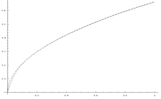
Figure 3 shows the results of applying the Algorithm 2 to this equation withn= 60.

5 Examples

In this section, we give examples of the Fredholm integral equations of the second kind. These examples show that the Algorithm 2 yields good results for a variety of kernels.

Example 1. Consider the following equation.

f(x) =x+

Z 1

−1

(4)

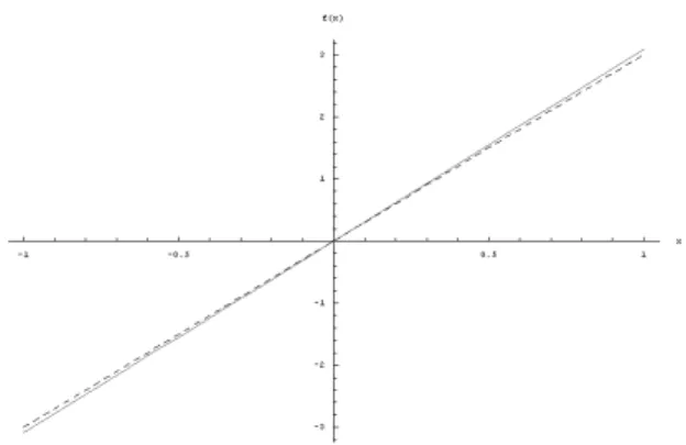
The exact solution to this equation is f(x) = 3x. By applying the Algorithm 2 to (13) with n = 40, the maximum error is 0.0075. Figure 4 compares the exact solution with the approximate one.

Example 2. Consider the following equation for 0 ≤

x≤1.

f(x) =x+

Z 1

0

k(x, y)f(y)dy, (14) where

k(x, y) =

x, x < y

y, x≥y . (15)

The exact solution to this equation is f(x) = sec 1 sinx. By applying the Algorithm 2 to (15) with n = 40, the maximum error is 0.0002. Figure 5 compares the exact solution with the approximate one.

Example 3. Consider the equation

f(x) +

Z 1

0

k(x, y)f(y)dy=xe+ 1, (16)

where

k(x, y) = min(x, y).

The exact solution to this equation is f(x) = exp(x). By applying the Algorithm 2 to (16) with n = 30, the maximum error is 0.00034. Figure 6 compares the exact solution with the approximate one.

f(x)−1₂ Z 1

−1

|x−y|f(y)dy=ex_. ₍₁₇₎

The exact solution to this equation is f(x) =

1 2xe

x ₊ _c

1ex + c2e−x, where c1 = c2 + (e 2

+ 1)−1

and c2 = (e 4

+ 6e2

+ 1)/8(e2

+ 1). By applying the Algorithm 2 to (17) with n= 50, the maximum error is 0.0037. Figure 7 compares the exact solution with the approximate one.

(5)

f(x) = sinx−x₂ +1 2

Z π₂

0

xyf(y)dy. (18)

The exact solution to this equation is f(x) = sinx. By applying the Algorithm 2 to (18) with n= 30, the max-imum error is 0.0005. Figure 8 compares the exact solu-tion with the approximate one.

6 Conclusion

This paper deals with the effective algorithms for solv-ing the Fredholm integral equation of the second kind. In fact, it provides the algorithms that implement the quadrature and its modification using Mathematica. It draws various examples of the Fredholm equations and shows that the algorithms yield acceptable results.

References

[1] Kythe, P.K., Puri, P., Computational Methods of Linear Integral Equations, Springer-Verlag, New York, 2002.

[2] Baker, C.T.H.,The Numerical Treatment of Integral Equations, Clarendon Press, Oxford, 1969.

[3] Huang, S.C., Shaw, R.P., “The Trefftz Method as an Integral Equation,”Adv. Eng. Software, V24, pp. 57-63, 1995.

[4] Yang, S.A., “An Investigation into Integral Equa-tion Methods Involving Nearly Singular Kernels for Acoustic Scattering,” J. Sound Vib. V23, N4, pp. 225-239, 2000.

[5] Abdou, M.A., “On the Solution of Linear and Non-linear Integral Equation,” Appl. Math. Comput., V14, N6, pp. 857-871, 2003.

[6] Jiang, S., Rokhlin, V., “Second Kind Integral Equa-tions for the Classical Potential Theory on Open Sur-face II,”J. Comput. Phys., V19, N5, pp. 1-16, 2004.

[7] Liang, D., Zhang, B., “Numerical Analysis of Graded Mesh Methods for a Class of Second Kind Integral Equations on Real Line,” J. Math. Anal. Appl., V29, N4, pp. 482-502, 2004.

[8] Babolian, E., Biazar, J., Vahidi, A.R., “The Decom-position Method Applied to Systems of Fredholm In-tegral Equations of the Second Kind,”Appl. Math. Comput., V14, N8, pp. 443-452, 2004.

[9] Maleknejad, K., Mahmoudi, Y., “Numerical Solu-tion of Linear Fredholm Integral EquaSolu-tions by Using Hybrid Taylor and Block-Pulse Functions,” Appl. Math. Comput., V14, N9, pp. 799-806, 2004.

[10] Maleknejad, K., Karami, M., “Using the WPG Method for Solving Integral Equations of the Second Kind,” Appl. Math. Comput., in press, doi:10.1016/j.amc.2004.04.109.

[11] Maleknejad, K., Karami, M., “Numerical So-lution of Non-linear Fredholm Integral Equa-tions by Using Multiwavelets in the Petrov-Galerkin Method,” Appl. Math. Comput., in press,doi:10.1016/j.amc.2004.08.047.

[12] Wu, W., Mathematics Mechanization, Science press and Kluwer Academic Publishers, Beijing, China, 2000.

[13] Chen, W., Lu, Z., “An Algorithm for Adomian De-composition Method,” Appl. Math. Comput., V15, N9, pp. 221-235, 2004.

[14] Wang, W., Lian, X., “A New Algorithm for Symbolic Integral with Application,” Appl. Math. Comput., V16, N2, pp. 949-968, 2005.

[15] Wang, W., Lin, C., “A New Algorithm for Inte-gral of Trigonometric Functions with Mechaniza-tion,” Appl. Math. Comput., V16, N4, pp. 71-82, 2005.

[16] Wang, W., “A New Algorithm for Solving DAEs with Mechanization,” Appl. Math. Comput., in press, doi:10.1016/j.amc.2004.08.010.

[17] Wang, W., “An Algorithm for Solving Non-linear Singular Perturbation Problems with Mechanization,” Appl. Math. Comput., in press, doi:10.1016/j.amc.2004.11.005.

[18] Wang, W., “Computations of Multi-Resultant with Mechanization,” Appl. Math. Comput., in press, doi:10.1016/j.amc.2004.11.034.